Improvement of the thermal and epithermal neutron scattering data for the interpretation of integral experiments

(1)

HAL Id: tel-01835720

https://tel.archives-ouvertes.fr/tel-01835720

Submitted on 11 Jul 2018

HAL is a multi-disciplinary open access

archive for the deposit and dissemination of sci-entific research documents, whether they are pub-lished or not. The documents may come from teaching and research institutions in France or abroad, or from public or private research centers.

L’archive ouverte pluridisciplinaire HAL, est destinée au dépôt et à la diffusion de documents scientifiques de niveau recherche, publiés ou non, émanant des établissements d’enseignement et de recherche français ou étrangers, des laboratoires publics ou privés.

Improvement of the thermal and epithermal neutron

scattering data for the interpretation of integral

experiments

Juan Scotta

To cite this version:

Juan Scotta. Improvement of the thermal and epithermal neutron scattering data for the interpretation of integral experiments. Nuclear Experiment [nucl-ex]. Université d’Aix-Marseille (AMU), 2017. English. �tel-01835720�

(2)

UNIVERSITE D’AIX-MARSEILLE

CEA Cadarache/ DEN / DER / SPRC / Laboratoire d’Etudes de Physiques

Thèse présentée pour obtenir le grade universitaire de docteur

Discipline : ED352 – PHYSIQUE ET SCIENCES DE LA MATIERE

Spécialité : Energie, Rayonnement et Plasma

Juan Pablo SCOTTA

Amélioration des données neutroniques de diffusion

thermique et epithermique pour l’interprétation des mesures

intégrales

Soutenue le 26/09/2017 devant le jury :

Luiz LEAL

IRSN

Examinateur

Cyrille DE SAINT JEAN

CEA Cadarache

Examinateur

Jose BUSTO

Université d’Aix Marseille

Examinateur

Florent REAL

Université de Lille

Rapporteur

Florencia CANTARGI

Centro Atomico Bariloche (ARG)

Rapporteur

Gilles NOGUERE

CEA Cadarache

Directeur de thèse

(3)

2

Abstract

In the present report it was studied the neutron thermal scattering of light water for reactors application. The thermal scattering law model of hydrogen bounded to the water molecule of the JEFF-3.1.1 nuclear data library is based on experimental measures performed in the sixties. The scattering physics of this latter was compared with a model based on molecular dynamics calculations developed at the Atomic Center in Bariloche (Argentina), namely the CAB model.

In the frame of this work, experimental measurements of the double differential cross sections were done at room temperature. The new microscopic data were used to analyze the performance of the CAB model and JEFF-3.1.1. The CAB model exhibits an improvement over JEFF-3.1.1.

The impact of these models was evaluated on application on reactor calculations at cold conditions. The selected benchmark was the MISTRAL program (UOX and MOX configurations), carried out in the zero power reactor EOLE of CEA Cadarache (France). The contribution of the neutron thermal scattering of hydrogen in water was quantified in terms of the difference in the calculated reactivity and the calculation error on the isothermal reactivity temperature coefficient (RTC).

For the UOX lattice, the calculated reactivity with the CAB model at 20 °C is +90 pcm larger than JEFF-3.1.1, while for the MOX lattice is +170 pcm because of the high sensitivity of the thermal scattering to this type of fuels. In the temperature range from 10 °C to 80 °C, the calculation error on the RTC is -0.27 ± 0.3 pcm/°C and +0.05 ± 0.3 pcm/°C obtained with JEFF-3.1.1 and the CAB model respectively (UOX lattice). For the MOX lattice, is -0.98 ± 0.3 pcm/°C and -0.72 ± 0.3 pcm/°C obtained with the JEFF-3.1.1 library and with the CAB model respectively. The results illustrate the improvement of the CAB model in the calculation of this safety parameter.

Finally, the uncertainties on the thermal scattering data were quantified creating covariance matrices between the parameters of the CAB model and the JEFF-3.1.1 library. The uncertainties were propagated to produce covariance matrices for the thermal scattering function and for the scattering cross section of hydrogen bounded to the light water. The uncertainty on the calculated reactivity of the MISTRAL benchmark (UOX fuel) is ±125 pcm for JEFF-3.1.1 and ±71 pcm for the CAB model (20 °C).

(4)

3

Résumé

Dans ces travaux de thèse, la diffusion thermique des neutrons pour l’application aux réacteurs à eau légère a été étudiée. Le modèle de loi de diffusion thermique de l’hydrogène lié à la molécule d’eau de la bibliothèque de données nucléaires JEFF-3.1.1 est basée sur des mesures expérimentales réalisées dans les années soixante. La physique de diffusion de neutrons de cette bibliothèque a été comparée à un modèle basé sur les calculs de dynamique moléculaire développé au Centre Atomique de Bariloche (Argentine), à savoir le modèle CAB.

Dans le cadre de ce travail, des mesures expérimentales de la section doublement différentielle ont été faites à température ambiante. Les nouvelles données microscopiques ont été utilisées pour analyser la performance du modèle CAB et du JEFF-3.1.1. Le modèle CAB présente une amélioration par rapport à JEFF-3.1.1.

L’impact de ces modèles a également été évalué sur le programme expérimental MISTRAL (configurations UOX et MOX) réalisé dans le réacteur de puissance nulle EOLE situé au CEA Cadarache (France). La contribution de la diffusion thermique des neutrons sur l’hydrogène dans l’eau a été quantifiée sur le calcul de la réactivité et sur l’erreur de calcul du coefficient de température isotherme (reactivity temperature Coefficient en anglais - RTC).

Pour le réseau UOX, l’écart entre la réactivité calculée à 20 °C avec le modèle CAB et celle du JEFF-3.1.1 est de +90 pcm, tandis que pour le réseau MOX, il est de +170 pcm à cause de la sensibilité élevée de la diffusion thermique pour ce type de combustible. Dans la plage de température de 10 °C à 80 °C, l’erreur de calcul sur le RTC est de -0.27 ± 0.3 pcm/°C avec JEFF-3.1.1 et de +0.05 ± 0.3 pcm/°C avec le modèle CAB pour le réseau UOX. Pour la configuration MOX, il est de -0.98 ± 0.3 pcm/°C et -0.72 ± 0.3 pcm/°C obtenu respectivement avec la bibliothèque JEFF-3.1.1 et avec le modèle CAB. Les résultats montrent l’apport du modèle CAB dans le calcul de ce paramètre de sureté.

Enfin, les incertitudes sur les données de diffusion thermique ont été quantifiées en calculant des matrices de covariance entre les paramètres du modèle CAB et ceux de la bibliothèque JEFF-3.1.1. Les incertitudes liés aux paramètres de modèle ont été propagées afin de calculer des matrices de covariance pour la loi de diffusion thermique et pour la section efficace de diffusion de l’hydrogène lié à l’eau légère. L’incertitude sur la réactivité calculée pour MISTRAL (réseau UOX) est de ±125 pcm pour JEFF-3.1.1 et ±71 pcm pour le modèle CAB (20 °C).

(5)

4

𝜇̅

to the CAB model parameters ... 132

7.4.2-Covariance matrix of the

𝜇̅

of the CAB model ... 132

7.5-Uncertainty propagation to the scattering function of JEFF-3.1.1 ... 135

7.6-Uncertainty propagation to the H1 in H2O scattering cross section of JEFF-3.1.1 ... 136

7.7-Uncertainty propagation to the mistral experiments ... 138

(9)

8

7.8.1-Uncertainty on the calculated reactivity by direct propagation of the leapr parameters

ffffffffffffffffffffffof JEFF-3.1.1 ... 139

7.8.2-Uncertainty propagation on the calculated reactivity using the ifp method ... 139

General conclusions and perspectives ... 144

List of references ... 147

Appendix A: MISTRAL-2 core used to compensate the reactivity loss due to the temperature ... 151

(10)

9

List of tables

1.1- Differences in reactivity ∆𝝆 = C - E (pcm) obtained with the thermal scattering laws of JEFF-3.1.1, CAB model and with the free gas approximation for the MISTRAL-1 configuration. The statistical uncertainty due to the Monte Carlo calculations is 2 pcm. The magnitude of the experimental

uncertainties ranges 200 pcm ... 21 3.1- IKE (JEFF-3.1.1) and CAB model parameters introduced in the LEAPR module for 1_{H in H}

2O at 294 K ... 38

3.2- Parameters of the TIP4P/2005f water potential ... 46 3.3- Water diffusion mass 𝑀𝑑𝑖𝑓𝑓 and molecular diffusion coefficient 𝐷 used in the CAB model at 294 K ... 47

4.1- Measured thermodynamic experimental conditions of water for the spectrometers IN4c (E0 = 14

meV) and IN6 (E0 = 3 meV) and the acquisition time in hours ... 60

4.2- Temperature and acquisition time measured at IN4c and IN6 spectrometers for the empty cell ... 61 5.1- Summary of the main characteristics of the three MISTRAL configurations ... 79 5.2- Excess of reactivity calculated with the TRIPOLI4 code for the MISTRAL-1 configuration at 20 °C. 

is the impact relative to the reference case of the official T4 library. The statistical uncertainty of

calculations is 4 pcm ... 84 5.3- Excess of reactivity calculated with the TRIPOLI4 code for the MISTRAL-1 configuration at 20 °C for

three cases. The statistical uncertainty of the calculations is 3 pcm ... 85 5.4- Differences in reactivity ∆𝜌 = C - E (pcm) obtained with the thermal scattering laws of JEFF-3.1.1

and CAB model for the MISTRAL-1, MISTRAL-2 and MISTRAL-3 configurations. In MISTRAL-1, the reactivity differences do not include the correction due to thermal expansion effects. The statistical

uncertainty due to the Monte Carlo calculations is 2 pcm ... 90 5.5- Polynomial coefficients 𝑎𝑖 provided by the CONRAD code after the least-square adjustment of the

∆𝜌 values reported in Table 4 with eq. (5). A quadratic polynomial fit was done for MISTRAL-1, while a

linear fit was proposed for MISTRAL-2 and MISTRAL-3 ... 91 5.6- Comparison of the polynomial coefficients 𝑎𝑖 provided by the CONRAD code after the least-square

adjustment of the ∆𝜌 values calculated for MISTRAL-1 with and without the thermal expansion effects

corrections. A linear fit is obtained when the reactivity corrections are taken into account ... 93 5.7- Ratio of JEFF-3.1.1 to CAB model of the absorption and scattering 1_{H in H}

2O reaction rates at 20°C

calculated in the MISTRAL experiments ... 95 5.8- Ratio of JEF-3.1.1 to CAB model of the capture to fission ratio of the three main fissile isotopes at

(11)

10 5.9- Summary of the calculation errors ∆𝛼𝑖𝑠𝑜(𝑇) for the MISTRAL experiments obtained with the

deterministic code APOLLO2 in association with the JEF-2.2 and JEFF-3.1.1 nuclear data libraries ... 97 5.10- Summary of the calculation errors ∆𝛼𝑖𝑠𝑜 (in pcm/°C) for the MISTRAL experiments obtained with

the Monte Carlo code TRIPOLI4. The present results are compared with those obtained with the deterministic code APOLLO2 [51]. The experimental uncertainties are also given in pcm/°C. The contribution of the statistical uncertainties due to the Monte Carlo calculations is negligible (± 0.02

pcm/°C) ... 98 5.11- Comparison of the calculation errors ∆𝛼𝑖𝑠𝑜 (in pcm/°C) for the MISTRAL-1 experiment applying

the thermal expansion corrections to the reactivity difference ∆𝜌 and to the reactivity temperature

coefficient difference ∆𝛼𝑖𝑠𝑜 ... 99

5.12- Differences in reactivity ∆𝜌 = C - E (pcm) obtained with the thermal scattering laws of JEFF-3.1.1 and CAB model and the 241_{Am evaluations of JEFF-3.1.1 and JEFF-3.2 libraries for the MISTRAL-2 and}

MISTRAL-3 configurations at 20 °C and 80 °C. The statistical uncertainty due to the Monte Carlo

calculations is 3 pcm ... 101 5.13- Differences in reactivity ∆𝜌 = C - E (pcm) obtained with the thermal scattering laws of JEFF-3.1.1

and CAB model and the 16_{O evaluations of JEFF-3.1.1 and JEFF-3.3 libraries for the 1,}

MISTRAL-2 and MISTRAL-3 configurations at MISTRAL-20 °C and 80 °C. The statistical uncertainty due to the Monte Carlo

calculations is 3 pcm ... 103 5.14- Excess of reactivity calculated with the TRIPOLI4 code for MISTRAL-1 at 20 °C for oxygen bound to

light water molecule and as a free gas. The statistical uncertainty of the calculations is 3 pcm ... 104 6.1- Parameters of the TIP4P/2005f water potential ... 111 6.2- Nuisance parameters for the experimental measures used in the retroactive analysis ... 115 6.3- Prior and posterior relative uncertainties and correlation matrix of the parameters of the

TIP4P/2005f water potential ... 116 6.4- Relative uncertainties and correlation matrix of the parameters of the TIP4P/2005f water potential

after the marginalization ... 118 6.5- JEFF-3.1.1 model parameters introduced in the LEAPR module for 1_{H in H}

2O at 294K ... 119

6.6- Relative uncertainties and correlation matrix of the LEAPR parameters of JEFF-3.1.1 after the

marginalization ... 125 7.1- Differences in reactivity ∆𝜌 = C - E (pcm) obtained with the thermal scattering laws of JEFF-3.1.1

and CAB model for the MISTRAL-1 and MISTRAL-2 configurations. In MISTRAL-1, the reactivity differences include the correction due to thermal expansion effects. The reported uncertainties on

(12)

11 each case are due to the CAB model parameters and to the LEAPR module parameters, in the case of JEFF-3.1.1, which were propagated with the CONRAD code. The combined statistical uncertainty due to

the Monte Carlo calculations is 25 pcm for the CAB model and 18 pcm for JEFF-3.1.1 ... 138 7.2- Comparison of the calculated uncertainty on the keff value of the PST-001.1 benchmark using

different uncertainty propagation methods. The reference case corresponds to the direct perturbation

(13)

12

List of figures

1.1- Total H2O cross section calculated with the CAB model and with the JEFF-3.1.1 library at 294 K ... 20

1.2- Radial cross section of MISTRAL-1 core from EOLE reactor ... 20 2.1- Hydrogen scattering and capture cross sections as a function of the neutron energy from JEFF-3.1.1

library ... 24 2.2- Continuous frequency spectra and intramolecular vibration modes of 1_{H H}

2O at 294 K for JEFF-3.1.1

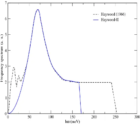
nuclear data library ... 31 3.1- Frequency spectra of 1_{H in H}

2O at 294 K measured by Haywood and modified by Koppel ... 39

3.2- Continuous frequency spectra of 1_{H in H}

2O at 294 K and 550 K as a function of the vibration energy

used in IKE model (ENDF/B-VII.1 and JEFF-3.1.1 nuclear data libraries) ... 39 3.3- Continuous component of the frequency spectrum of 1_{H in H}

2O at 294 K of the nuclear data

libraries ENDF/B-VII.1 and JEFF-3.1.1 ... 40 3.4- Simulation of 512 H2O molecules with GROMACS code in a cubic box of side a = 2.48 nm ... 42

3.5- VACF of H(H2O) (continuous red line) and O(H2O) (dash blue line) at 294 K generated with the

molecular dynamic simulations code GROMACS and the water potential TIP4P/2005f ... 45 3.6- Generalized frequency spectrum of H(H2O) (left scale), O(H2O) (right scale) and H2O (left scale) at

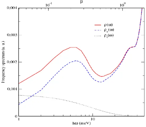
294 K ... 45 3.7- Low energy detail of the generalized frequency (continuous line), continuous (dash line) and

diffusive spectrum (dotted line) from Egelstaff-Schofield model of 1_{H H}

2O at 294 K ... 47

3.8- CAB model (continuous red line) and JEFF-3.1.1 (dash blue line) continuous frequency spectra and intramolecular vibration modes of 1_{H H}

2O at 294 K as a function of the excitation energy (lower scale)

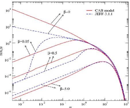
and dimensionless energy transfer (upper scale) ... 48 3.9- S() as a function of the momentum transfer for CAB model and JEFF-3.1.1 nuclear data library

at 294 K ... 49 3.10- Symmetric S() as a function of the momentum transfer for CAB model and JEFF-3.1.1 nuclear

data library at 294 K ... 49 3.11- Double differential scattering cross section for light water calculated with CAB model and

JEFF-3.1.1 compared with data measured by Novikov (1986), for E0 = 8 meV,  = 37° and T = 294 K. The

(14)

13 3.12- Double differential scattering cross section for light water calculated with CAB model and JEFF-3.1.1 compared with data measured by Bischoff (1967), for E0 = 231 meV,  = 25° and T = 294 K. The

energy resolution is 5% ... 51

3.13- 1_{H in H} 2O scattering cross section calculated with CAB model and JEFF-3.1.1 at 294 K (upper plot). The ratio between JEFF-3.1.1 and CAB model is in the bottom plot ... 52

3.14- Total H2O cross section calculated with CAB model and JEFF-3.1.1 at 294 K ... 53

3.15- Double differential scattering cross section calculated with 1_{H in H} 2O of CAB model and 16O in the free gas approximation compared with 1_{H in H} 2O and 16O in H2O of CAB model, for E0 = 231 meV,  = 25° and T = 294 K ... 55

3.16- Scattering cross sections of 16_{O in H} 2O calculated with CAB model and 16O calculated in the free gas approximation of JEFF-3.1.1 at 294 K (upper plot). The ratio between JEFF-3.1.1 and CAB model is in the bottom plot ... 55

4.1- The IN4c time-of-flight spectrometer ... 58

4.2- The IN6 time-of-flight spectrometer ... 59

4.3- Characteristics of the Cu-Be sample holder ... 59

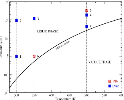
4.4- Water pressure – temperature diagram showing the thermodynamic states measured for IN4c (blue full squares) and IN6 (red squares) spectrometers ... 60

4.5- Vanadium intensity measured at IN4c spectrometer for  = 14° (upper plot) and  = 120° (lower plot) ... 62

4.6- Vanadium intensity measured at IN6 spectrometer for  = 11° (upper plot) and  = 115° (lower plot) ... 62

4.7- Half-width at half-maximum of the vanadium elastic peak as a function of the scattering angle ... 63

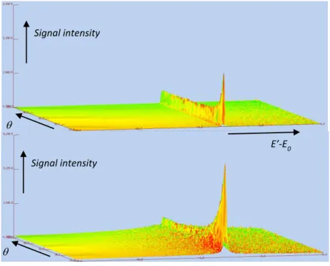
4.8- Intensity of the water signal and empty cell as a function of  and E’-E0 (upper plot) and intensity of the empty cell measure (lower plot) for IN4c at 300 K... 64

4.9- Intensity of the water signal and empty cell as a function of  and E’-E0 (upper plot) and intensity of the empty cell measure (lower plot) for IN6 at 350 K ... 65

4.10- Intensity of the “H2O+sample holder” and “sample holder” as a function of E’-E0 for 𝜃 = 15° measured in IN4c spectrometer at 300 K (left plot). Detail of the quasi-elastic peaks (right plot)... 66

4.11- Intensity of the “H2O+sample holder” and “sample holder” as a function of E’-E0 for 𝜃 = 15° measured in IN6 spectrometer at 350 K (left plot). Detail of the quasi-elastic peaks (right plot) ... 67

4.12- Water double differential scattering cross section at E0 = 14 meV and  = 15° and 45°, measured in IN4c spectrometer at 300 K. Detail of the quasi-elastic peaks (right plot) ... 68

(15)

14 4.13- Water double differential scattering cross section at E0 = 3 meV and  = 15° and 45°, measured in

IN6 spectrometer at 350 K. Detail of the quasi-elastic peaks (right plot) ... 69

4.14- Simplified ToF model implemented in TRIPOLI4 code. E0 designated the incident neutron energy,  the scattering angle, L the flight path distance and E’ the secondary energy ... 70

4.15- Comparison between the unbroadened (dashed curve) and broadened (continuous curve) double differential cross sections calculated with the Monte Carlo code TRIPOLI4 for E0 = 14 meV,  = 15° and 300 K. The convolution was done with the experimental vanadium measures ... 71

4.16- Double differential scattering cross section at E0 = 14 meV,  = 15° and 300 K calculated with JEFF-3.1.1, CAB model and Free gas model compared with the experimental data ... 71

4.17- Double differential scattering cross section at E0 = 3 meV,  = 15° and 350 K calculated with JEFF-3.1.1 and CAB model compared with the experimental data ... 72

4.18- Comparison of two convolution options for E0 = 14 meV (IN4c),  = 15° and T = 300 K. The dashed line was obtained convoluting the double differential cross section with a Gaussian function of 1.44% of resolution. The continuous line was obtained convoluting with the vanadium measures ... 73

4.19- Double differential scattering cross section at E0 = 3 meV,  = 45° and 350 K calculated with CAB model compared with the experimental data ... 74

4.20- 𝑆(𝑞̅, 𝜔) for 𝑞̅ = 1.6𝐴̇−1 at 294 K (left hand plot) obtained using the quantum correction (GAAQC) and the Gaussian approximation. In the right hand plot it was calculated the double differential cross section for 𝐸0 = 3 meV, 𝜃 = 71° and 294 K using both approaches ... 75

5.1- Radial cross section of MISTRAL-1 core ... 78

5.2- Radial cross section of MISTRAL-2 core. The configuration corresponds to 20°C ... 78

5.3- Radial cross section of MISTRAL-3 core ... 78

5.4- Flowchart of the calculation scheme used to produce the thermal scattering libraries for TRIPOLI4 ... 81

5.5- Effective temperature correction to the temperature for taking into account the crystal lattice effects in the fuel matrix ... 81

5.6- Reactivity corrections as a function of the temperature due to the thermal expansion of the MISTRAL-1 core. The reference corresponds to reactivity at 20 °C. The solid line represents the linear fit ... 83

5.7- Energy ranges for the tests performed over MISTRAL-1 configuration at 20 °C ... 85

5.8- 1_{H scattering cross sections bound to H} 2O at 294 and in the free gas approximation at 294 K and 1250 K from JEFF-3.1.1 library ... 86

5.9- Interpolation of the model parameters established by Mattes and Keinert between 6 °C and 80 °C ... 87

5.10- Continuous frequency spectra for 1_{H in H} 2O interpolated over a fine temperature mesh ... 88

(16)

15 5.11- Total cross section of 1_{H in H}

2O calculated with the broad temperature mesh of the JEFF-3.1.1

library (20 °C, 50 °C and 100 °C) and interpolated over a fine temperature mesh (from 6 °C to 80 °C) ... 88

5.12- Differences in reactivity ∆𝜌(𝑇) obtained with the thermal scattering laws of JEFF-3.1.1 and CAB model for the MISTRAL-1, MISTRAL-2 and MISTRAL-3 configurations. The solid lines represent the best fit curves calculated with the CONRAD code ... 92

5.13- Differences in reactivity ∆𝜌(𝑇) obtained with the thermal scattering laws of JEFF-3.1.1 and CAB model for the MISTRAL-1 with (empty points) and without (filled points) the thermal expansion effects ... 93

5.14- H2O cross section calculated with CAB model and JEFF-3.1.1 at 293.6 K, together with the MISTRAL-2 neutron spectrum at the same temperature ... 95

5.15- Calculation errors on the reactivity temperature coefficient as a function of the temperature for the MISTRAL-1 experiment. The uncertainty bands accounts for the statistical uncertainty of the Monte Carlo calculations ... 99

5.16- Comparison between the 241_{Am capture cross sections as a function of the energy of JEFF-3.1.1} and JEFF-3.2 libraries at 294 K, together with the MISTRAL-2 neutron spectrum at 20 °C and 80 °C ... 101

5.17- Comparison between the 241_{Am capture cross sections as a function of the energy of JEFF-3.1.1} and JEFF-3.2 libraries at 294 K, together with the MISTRAL-2 neutron spectrum at 20 °C and 80 °C ... 103

6.1- Total cross section measurements at 294 K used in the fitting procedure of the GLSM ... 112

6.2- Average cosine of the scattering angle measurements at 294 K used in the fitting procedure of the GLSM ... 112

6.3- Transmission data measured at 294 K ... 114

6.4- Full correlation matrix between the model and the experimental parameters after marginalization ... 117

6.5- Continuous distribution and discrete oscillators used in JEFF-3.1.1 at 294 K ... 118

6.6- Effect on the H2O total cross section of the scaling factor applied to the vibration energy grid used to reconstruct the frequency distribution at 294 K ... 120

6.7- H2O total cross section measurements at 294 K from the EXFOR database compared to the cross section of JEFF-3.1.1 (upper plot) and the transmission data converted using a generic areal density of 0.017 barn-1_{... 121}

6.8- Modifications of the low energy part of a given theoretical transmission of a thick water sample according to the diffusion constant 𝑐 ... 122 6.9- Bending and stretching modes calculated at 294 K with the molecular dynamic code GROMACS and

(17)

16 compared with the energies of the first and second oscillators introduced in JEFF-3.1.1 (205.0 meV and

436.0 meV) ... 123

7.1- 𝑆(𝛼, 𝛽0) and the multigroup 𝑆̅(𝛼, 𝛽0) as a function of the momentum transfer for 𝛽0= 1.0 calculated with the CAB model at 294 K ... 129

7.2- Sensitivities of the 𝑆̅(𝛼, 𝛽0) function (dashed line) to the CAB model parameters as a function of the momentum transfer for 𝛽0= 1.0 calculated with the CAB model at 294 K ... 129

7.3- Relative uncertainties and correlation matrix of the 𝑆̅(𝛼, 𝛽0) function for 𝛽0= 1.0 (upper plot) and 𝛽0= 10.0 (bottom plot) calculated with the CAB model at 294 K ... 130

7.4- Sensitivity of the 1_{H in H} 2O scattering cross section at 294 K to the TIP4P/2005f water potential parameters. The dashed line represents the scattering cross section of 1_{H in H} 2O ... 131

7.5- Relative uncertainties and correlation matrix of the 1_{H in H} 2O scattering cross section calculated with the CAB model at 294 K. The left hand plot shows the results after the fitting procedure and the right hand plot the results after the marginalization. For both cases the calculated cross section and the uncertainty bands are plotted with the experimental data used in the retroactive analysis ... 133

7.6- Sensitivity of the 𝜇̅ the TIP4P/2005f water potential parameters. The dashed line represents the calculation done with CAB model at 294 K ... 134

7.7- Relative uncertainties and correlation matrix of average cosine of the scattering angle 𝜇̅ calculated with the CAB model at 294 K. The right plot represents the calculated 𝜇̅ and the uncertainty bands compared with the experimental data used in the retroactive analysis ... 134

7.8- Relative uncertainties and correlation matrix of the 𝑆̅(𝛼, 𝛽0) function for 𝛽0= 1.0 (upper plot) and 𝛽0= 10.0 (lower plot) calculated with the JEFF-3.1.1 library at 294 K ... 136

7.9- Relative uncertainties and correlation matrix of the 1_{H in H} 2O scattering cross section calculated with the JEFF-3.1.1 library at 294 K after the marginalization... 137

7.10- Comparison of the total cross section calculated with the CAB model and the JEFF-3.1.1 library at 294 K around the thermal neutron energy ... 137

7.11- Sensitivity profiles of the keff value to the multigroup 𝑆̅(𝛼0, 𝛽) for 𝛼0= 0.5 (left hand plot) and to the 𝑆̅(𝛽) (right hand plot) calculated at 294 K ... 140

7.12- Relative uncertainties and correlation matrix of the scattering function 𝑆̅(𝛽) averaged in one momentum transfer group at 294 K ... 141

A.1- MISTRAL-2 configuration at 10 °C and 15 °C ... 151

A.2- MISTRAL-2 configuration at 20 °C ... 151

(18)

17

(19)

18

Chapter 1 Introduction

1.1 Context

The knowledge of the neutron distribution in space, energy and time is crucial to understand the behavior of a nuclear reactor and critical systems as well. In principle, the time-dependent Boltzmann’s neutron transport equation predicts the distribution of the neutrons with the appropriate initial and boundary conditions [1]: 𝟏 𝒗 𝝏 𝝏𝒕𝝋(𝒓̅, 𝜴, 𝑬, 𝒕) = ∬ 𝜮𝒔(𝑬 ′_{, 𝜴}′_{→ 𝑬, 𝜴) 𝝋(𝒓̅, 𝜴′, 𝑬′, 𝒕)𝒅𝑬}′_𝒅𝜴′₊𝝌(𝑬) 𝟒𝝅 ∫ 𝝂(𝑬 ′_{) 𝜮} 𝒇(𝑬′)𝝋(𝒓̅, 𝜴′, 𝑬′, 𝒕)𝒅𝑬′ + 𝑸(𝒓̅, 𝜴, 𝑬, 𝒕) − 𝜮𝒕𝝋(𝒓̅, 𝜴, 𝑬, 𝒕) − 𝜴 ∙ 𝜵̅𝝋(𝒓̅, 𝜴, 𝑬, 𝒕) (𝟏)

where 𝒗 is the neutrons velocity, 𝝋 is the angular flux, 𝜮𝒔, 𝜮𝒇 and 𝜮𝒕 are the macroscopic scattering,

fission and total cross sections, 𝝌 is the fission spectrum, 𝝂 is the mean number of neutrons emitted per fission and 𝑸 is the external source factor.

This integral-differential equation reflects the balance of neutrons at any time, energy and space due to their appearances and disappearances. The first term of the right part of the equation, are the scattered neutrons from an energy and solid angle 𝑬′_,_𝜴′_to_𝑬_,_𝜴_{. The second term reflects the neutrons}

created by fission. The third term describes a neutron source. The fourth term defines the neutrons disappearance due to absorption or to scattering. The last term expresses the neutrons lost by leakages.

The neutrons produced by the fission of fissile isotopes have a very high energy (typically of 2 MeV). In order to increase the probability of producing more fissions, they need to be lose energy in a process called slowing-down. The first term of the right part of the equation models this physical process.

The materials used as moderators, consist of atoms bonded together chemically or in a crystalline structure. For neutron energies higher than the bonding energy of these atoms the interaction of neutrons with the material can be approximated by a free gas interaction. For smaller energies (typically below 1 eV), the target molecule motion must be accounted as a whole in order to reproduce correctly the physics of the scattering process.

The light water is one of the most used materials as moderators and coolants for nuclear reactors and critical systems in general. From a safety point of view, the correct understanding of the interaction of the neutron with the water molecule is very important to predict their transport. The neutron scattering process in light water is the object of study in the present work.

(20)

19

1.2 Motivations

When performing neutron transport calculation, reactor calculation codes need the microscopic cross sections of the isotopes involved in the system to predict the nuclear reactions. The nuclear data information is obtained through cross section libraries that are carefully constructed on the basis of nuclear data evaluation process. These libraries are commonly referred as the Evaluated Nuclear Data files (ENDF).

The nuclear data libraries ENDF/B-VII.1 [2] and the JEFF-3.1.1 library [3] contain a model that describes the thermal neutron scattering with the light water. This model, namely IKE model [4] is based on experimental measurements done in the sixties (almost 50 years ago).

Nowadays, the calculation power of computers enables producing more accurate and reliable theoretical models with a completely different approach like molecular dynamic simulation. The methodology consists of simulating in a microscopic scale the interaction forces between the water molecules. In this context, a new model was developed by the neutron physics research group of Centro Atomico Bariloche (Argentina): the CAB model [5].

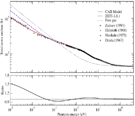
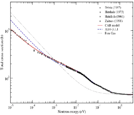
Figure 1.1 compares the H2O total cross section calculated with the CAB model (continuous line), with

the JEFF-3.1.1 nuclear data library (dashed line), and in the free gas approximation (dotted line) for an energy range of 10-5_{eV to 5 eV at 294 K.}

The importance of taking into account the chemical bond of the hydrogen with the oxygen, at this energy range, is pointed out when one compares the cross section of 1_{H as a free gas with the}

experimental data. The agreement is poor. The cross sections calculated with a model describing the scattering of a neutron with the 1_{H bounded to the H}

2O molecule are represented by the JEFF-3.1.1 and

the CAB model. In both cases, the trends of the total cross sections are consistent with the experimental data up to approximately 0.1 meV. Below this energy, the differences between JEFF-3.1.1 and the CAB model are clearly marked. The ratio between the cross sections is close to 1.54 at 10-5_eV.

The impact of such differences in the total cross sections between the free gas approximation and the thermal scattering models is illustrated in a reactor calculation. As a matter of comparison, we chose the MISTRAL-1 experiment at 20 °C, which was carried out in the EOLE reactor at CEA Cadarache. The MISTRAL-1, shown in Figure 2.1, is a homogeneous UO2 configuration moderated and cooled by light water (a detailed analysis of this experiment will be described in the present report). It was calculated the reactivity with the Monte Carlo code TRIPOLI4, replacing the evaluated file of 1_{H in H}

2O of

JEFF-3.1.1 library by the 1_{H in H}

2O of CAB model and the 1H in the free gas approximation. The reactivity

difference, ∆𝜌, between the calculated (C) and the experimental (E) reactivity for each case are listed in table 1.1.

The reactivity difference between the JEFF-3.1.1 and CAB model cases is 90 pcm. The origin of such discrepancy will be studied further. The remarkable outcome of this analysis is the overestimation of the reactivity by the 1_{H free gas approximation in almost 1000 pcm. The difference with respect to}

(21)

20 200 pcm, it is confirmed the significance of taking into account the hydrogen bounded to water molecule in thermal scattering.

Fig. 1.1 Total H2O cross section calculated with the CAB model and with the JEFF-3.1.1 library at 294 K.

(22)

21 Table 1.1. Differences in reactivity ∆𝜌 = C - E (pcm) obtained with the thermal scattering laws of JEFF-3.1.1, CAB model and with the free gas approximation for the MISTRAL-1 configuration. The statistical uncertainty due to the Monte Carlo calculations is 2 pcm. The magnitude of the experimental uncertainties ranges 200 pcm. Moderator ∆𝝆 = C - E (pcm) 1_{H in H} 2O of JEFF-3.1.1 192 1_{H in H} 2O of CAB model 283 1_{H as free gas} ₉₆₂

1.3 Objectives

The first key point in the present study is to analyze the behavior of the two models and study the feasibility of producing thermal neutron scattering data calculated by means of molecular dynamics.

The second issue is to evaluate and quantify the uncertainties of the two models. None of the existing nuclear data libraries provides the uncertainties for the thermal scattering data of light water. A correct estimation of the uncertainties on the nuclear data, in general, enables determining the safety margins of a critical system.

1.4 Report description

The chapter 2 is dedicated to explain the thermal neutron scattering theory which sets the background for the present report. It also presents the evaluation methodology of the scattering function, which is done with the LEAPR module of the processing code NJOY.

In the chapter 3, the models IKE and CAB will also be presented. The behavior of the models is characterized microscopically, studying the frequency spectrum of hydrogen in light water, the double differential and total cross sections.

The chapter 4 describes the neutron time-of-flight experiment carried out at Laue-Langevin Institute (Grenoble, France), where it was measured the double differential cross section of light water at cold rector operating conditions. A Monte Carlo simulation was done to evaluate the agreement of the thermal scattering models with the new experimental data.

In the chapter 5, the thermal scattering laws of light water are compared macroscopically in integral calculations. It is evaluated their impact on an integral experiment at cold reactor operating conditions. The MISTRAL experimental program performed at EOLE reactor (France) was selected as benchmark.

(23)

22 Chapter 6 covers the methodology for evaluating and quantifying the uncertainties due to the thermal neutron scattering with light water. Firstly, the framework regarding the uncertainty treatment is explained and secondly, the approach for producing covariances is presented.

Finally, propagation of the uncertainties due to the thermal scattering data are presented in chapter 7. Covariance matrices of the thermal scattering function and the scattering cross section of hydrogen in light water were produced. The impact of the uncertainty of the calculated reactivity in the MISTRAL benchmark was studied as well.

(24)

23

Chapter 2 Thermal neutron scattering

The present chapter is devoted to the theory of neutron scattering. Firstly and taking as a reference bibliography [6], the basic notions of neutron scattering are presented. Later on, it is explained how the thermal scattering function is evaluated using the LEAPR module of NJOY processing code [7].

2.1 Introduction to thermal neutron scattering theory

In the low neutron energy range, typically below 5 eV, neutron scattering is affected by the atomic bonding of the scattering molecule in the moderator. Compared to a free nucleus, this changes the reaction cross section and, thus, the energy and angular distribution of the secondary neutrons.

Neutron scattering is classified as elastic and inelastic scattering. While the former is important, the latter has direct link to the reactor applications because neutrons need to slow down to increase the fission probability of the fissile isotopes. Both elastic and inelastic scattering can be coherent or incoherent. In coherent scattering, the interference phenomena between the waves reflected by close nuclei affect the scattering target. However, in the particular case of light water the scattering process can be treated as pure incoherent as it will be seen further in the chapter.

The H2O total microscopic cross section of thermal neutrons is given by:

𝜎_𝑡𝐻2𝑂_{(𝐸) = 2𝜎}

𝑡𝐻(𝐸) + 𝜎𝑡𝑂(𝐸), (1)

where 𝜎𝑡𝑂 is the total cross section of 16O and 𝜎𝑡𝐻 is the total cross section of 1H. The latter is given by

𝜎𝑡𝐻(𝐸) = 𝜎𝛾(𝐸) + 𝜎𝑛(𝐸). (2)

In the thermal energy range, the capture cross section 𝜎𝛾(𝐸) can be approximated as:

𝜎𝛾(𝐸) = 𝜎𝛾0√

𝐸0

𝐸, (3)

where 𝜎𝛾0 is the capture cross section measured at the thermal neutron energy 𝐸0= 25.3 meV.

Figure 2.1 compares the scattering cross section at T = 0 K and 294 K with the capture cross section of hydrogen as given in the nuclear data library JEFF-3.1.1. For a given temperature the cross section is broadened using the processing code NJOY [R. E. MacFarlane et al., The NJOY Data Processing System, Version 2012, Los Alamos National Laboratory (2012)].

(25)

24 Fig. 2.1 Hydrogen scattering and capture cross sections as a function of the neutron energy from JEFF-3.1.1 library.

In the case of hydrogen bonded to the water molecule, the inelastic scattering cross section 𝜎𝑛 is

related to the double differential cross section as:

𝜎𝑛(𝐸) = ∬

𝑑2_𝜎 𝑛

𝑑𝛺𝑑𝐸′𝑑𝐸

′_{𝑑Ω. (4)}

For simplicity, the subscript 𝑛 in the scattering cross section 𝜎𝑛 will be omitted from now on.

The double differential cross section expresses the probability that an income neutron flux of energy E and direction  will be scattered by a target at a secondary energy E’ and direction ’ [6]:

𝑑2_𝜎 𝑑𝛺𝑑𝐸′= 1 4𝜋𝑘𝐵𝑇 √𝐸′ 𝐸 𝑒 −𝛽 2 _(𝜎_𝑐𝑜ℎ_{𝑆(𝛼, 𝛽) + 𝜎}_𝑖𝑛𝑐_𝑆_𝑠_{(𝛼, 𝛽)), (5)}

where 𝜎𝑐𝑜ℎ and 𝜎𝑖𝑛𝑐 are respectively the coherent and incoherent scattering cross sections, 𝑘𝐵 is the

Boltzmann constant and 𝑇 is the temperature of the material.

The 𝑆(𝛼, 𝛽) function is the thermal scattering function, which is given by:

𝑆(𝛼, 𝛽) = 𝑆𝑠(𝛼, 𝛽) + 𝑆𝑑(𝛼, 𝛽), (6)

where 𝑆𝑠(𝛼, 𝛽) is the self-scattering function that accounts for non-interference or incoherent effects,

and 𝑆𝑑(𝛼, 𝛽) is the distinct-scattering function that accounts for interference or coherent effects.

(26)

25 𝛼 =𝐸 ′_{+ 𝐸 − 2√𝐸}′_𝐸𝜇 𝐴𝑘𝐵𝑇 , (7) 𝛽 =𝐸 ′_{− 𝐸} 𝑘𝐵𝑇 = ℏ𝜔 𝑘𝐵𝑇 , (8)

where 𝜇 is the cosine of the scattering angle in the laboratory system and 𝐴 is the ratio between the mass of the scattering target 𝑀 and the neutron mass 𝑚. The energy transfer 𝐸′− 𝐸 is sometimes denoted as the product between the reduced Planck’s constant ℏ and the excitation frequency 𝜔.

In the literature, the scattering function might be expressed as a function of other variables rather than the dimensionless momentum and energy transfer 𝛼, 𝛽. If 𝑞̅ is the neutron wave vector change, then the scattering law can be expressed as:

𝑆(𝑞̅, 𝜔) = 𝑆(𝛼, 𝛽)𝑒

ℏ𝜔 2𝑘𝐵𝑇

𝑘𝐵𝑇

. (9)

The module of the wave vector change 𝑞̅ is related to the dimensionless momentum transfer 𝛼 as:

𝑞2= |𝑘̅ − 𝑘̅′|2=2𝑚

ℏ2 (𝐸′+ 𝐸 − 2𝜇√𝐸𝐸′). (10)

From eq. (7) we have then:

𝑞2₌2𝑀𝑘𝐵𝑇

ℏ2 𝛼. (11)

Expressing the scattering function as 𝑆(𝑞̅, 𝜔) can be especially useful when performing experimental measurements, as one obtains direct information of the transferred energy and angle of the scattered neutrons. In practice, the 𝛼 and 𝛽 variables are used for the evaluation of the scattering function with the LEAPR module as it will be seen later.

The next sections will be devoted to explain how to calculate the coherent and the incoherent cross sections and the self and distinct scattering functions using the formalism introduced by L. Van Hove in 1954 [9]. Next, the subject will be focused on light water, and to the way the scattering function is obtained using the processing code NJOY.

2.2 The coherent and incoherent cross sections

It can be shown [6] that at low neutron energy, the cross section in scattering of neutrons with a single fixed nucleus is given by:

𝜎𝑛= 4𝜋𝑏2. (12)

The parameter 𝑏 is known as the scattering length. It depends on the target nucleus and the spin state of the nucleus-neutron system. If the nucleus has a spin 𝐼, the combined system can have a spin 𝐼 ±

(27)

26 1/2 (the neutron spin is 1/2). Each spin state has its own value of 𝑏. There will be then two possible values of the scattering length for that particular nucleus. The exceptions are nuclei with spin zero, where the scattering will be purely coherent as it will be demonstrated further on this chapter.

Considering a scattering system of a single element where the scattering length varies from one nucleus to another, then the average value of 𝑏 for the whole system is:

𝑏̅ = ∑ 𝑓𝑖𝑏𝑖 𝑖

. (13)

The relative frequencies 𝑓𝑖 denote the probability of a system to have a scattering length 𝑏𝑖. If 𝑏+ is the

scattering length given by the spin of the system neutron-nucleus 𝐼 + 1/2 and 𝑏− the one given by the spin 𝐼 − 1/2, then the number of states associated with each spin will be respectively:

2 (𝐼 +1

2) = 2𝐼 + 2. (14)

2 (𝐼 −1

2) = 2𝐼 − 1. (15) If the neutrons are unpolarized and the nuclear spins are randomly orientated (no correlation between the scattering lengths of different nuclei), then each spin is equiprobable. Eq. (13) turns into:

𝑏̅ = 𝑓+𝑏++ 𝑓−𝑏−= 2𝐼 + 2 2𝐼 + 2 + 2𝐼𝑏 +₊ 2𝐼 2𝐼 + 2 + 2𝐼𝑏 −₌ 𝐼 + 1 2𝐼 + 1𝑏 +₊ 𝐼 2𝐼 + 1𝑏 −_{. (16)}

A generalization can be made assuming that there are different isotopes in the scattering system. Then the frequencies 𝑓+ and 𝑓− are multiplied by the relative abundance of the isotope 𝜁𝑖:

𝑏̅ = ∑ 𝜁𝑖 𝑖 (𝐼𝑖+ 1 2𝐼𝑖+ 1 𝑏𝑖++ 𝐼𝑖 2𝐼𝑖+ 1 𝑏𝑖− ). (17)

The microscopic coherent and incoherent cross sections are defined as:

𝜎𝑐𝑜ℎ= 4𝜋(𝑏̅) 2 , (18) 𝜎𝑖𝑛𝑐= 4𝜋 [𝑏̅̅̅ − (𝑏̅)2 2 ], (19)

where the average value of the square of the scattering length is:

𝑏2

̅̅̅ = ∑ 𝑓_𝑖𝑏𝑖2 𝑖

. (20)

Considering that the potential interaction between the neutron and the system is given by the “Fermi Pseudo potential”, which essentially is a delta function in space, and following the notation in [6], the double differential cross section can be expressed as the sum of the coherent and the incoherent double differential cross sections:

(28)

27 𝑑2𝜎 𝑑𝛺𝑑𝐸′= ( 𝑑2𝜎 𝑑𝛺𝑑𝐸′)_𝑐𝑜ℎ+ ( 𝑑2𝜎 𝑑𝛺𝑑𝐸′)_𝑖𝑛𝑐, (21) 𝑑2𝜎 𝑑𝛺𝑑𝐸′= 𝑘′ 𝑘 (𝑏̅)2 2𝜋ℏ ∑ ∫ < 𝑗 ′_{, 𝑗 > 𝑒}−𝑖𝜔𝑡_𝑑𝑡 𝑗𝑗′_{;𝑗′≠𝑗} +𝑘′ 𝑘 𝑏2 ̅̅̅ 2𝜋ℏ∑ ∫ < 𝑗, 𝑗 > 𝑒 −𝑖𝜔𝑡_𝑑𝑡 𝑗 , (22)

where the internal product < 𝑗′, 𝑗 > is defined as:

< 𝑗′, 𝑗 >=< 𝑒𝑥𝑝 (−𝑖𝑞̅ ∙ 𝑅̅_𝑗′(0)) 𝑒𝑥𝑝 (𝑖𝑞̅ ∙ 𝑅̅_𝑗(𝑡)) > , (23)

where 𝑘̅ and 𝑘′̅ are the incident and final neutron wave vectors, 𝑅̅ (𝑗 = 1, … , 𝑁) the position vector of 𝑗

the jth_{nucleus in the scattering system of N nuclei.}

Multiplying and dividing eq. (22) by the factor 4𝜋 we can express explicitly the double differential cross section as a function of 𝜎𝑐𝑜ℎ and 𝜎𝑖𝑛𝑐 :

( 𝑑 2_𝜎 𝑑𝛺𝑑𝐸′) 𝑐𝑜ℎ = 𝜎𝑐𝑜ℎ 1 4𝜋 𝑘′ 𝑘 1 2𝜋ℏ∑ ∫ < 𝑒𝑥𝑝 (−𝑖𝑞̅ ∙ 𝑅̅𝑗′(0)) 𝑒𝑥𝑝 (𝑖𝑞̅ ∙ 𝑅̅𝑗(𝑡)) > 𝑒 −𝑖𝜔𝑡_𝑑𝑡 𝑗′𝑗 . (24) ( 𝑑 2_𝜎 𝑑𝛺𝑑𝐸′)_𝑖𝑛𝑐 = 𝜎𝑖𝑛𝑐 1 4𝜋 𝑘′ 𝑘 1 2𝜋ℏ∑ ∫ < 𝑒𝑥𝑝 (−𝑖𝑞̅ ∙ 𝑅̅𝑗(0)) 𝑒𝑥𝑝 (𝑖𝑞̅ ∙ 𝑅̅𝑗(𝑡)) > 𝑒 −𝑖𝜔𝑡_𝑑𝑡 𝑗 . (25)

It can be seen from eq. (22) that the coherent scattering depends on the correlation between the positions of the same nuclei at different times, and on the correlation between the positions of different nuclei at different times. The incoherent scattering depends only on the correlation between the positions of the same nuclei at different times. This is the reason why the coherent component arises interference effects.

2.3 The coherent and incoherent scattering functions

Following the mathematical formulation of the scattering introduced by Van Hove in 1954 [9], we define firstly the intermediate scattering function 𝐼(𝑞̅, 𝑡) as:

𝐼(𝑞̅, 𝑡) = ∑ < 𝑒𝑥𝑝 (−𝑖𝑞̅ ∙ 𝑅̅_𝑗′(0)) 𝑒𝑥𝑝 (𝑖𝑞̅ ∙ 𝑅̅_𝑗(𝑡)) >

𝑗′𝑗

. (26)

Secondly, we define the time dependent pair correlation function 𝐺(𝑟̅, 𝑡) by:

𝐺(𝑟̅, 𝑡) = 1

(2𝜋)3∫ 𝐼(𝑞,̅ 𝑡). 𝑒−𝑖𝑞̅∙𝑟̅𝑑𝑞̅ . (27)

And finally, the scattering function of the system is defined as the Fourier transform in time of the intermediate scattering function:

(29)

28 𝑆(𝑞̅, 𝜔) = 1

2𝜋ℏ∫ 𝐼(𝑞,̅ 𝑡). 𝑒

−𝑖𝜔𝑡_{𝑑𝑡. (28)}

Arranging the expressions, we derive the scattering function as the Fourier transform in space and time of the time dependent pair correlation function 𝐺(𝑟̅, 𝑡):

𝑆(𝑞̅, 𝜔) = 1

2𝜋ℏ∫ ∫ 𝐺(𝑟,̅ 𝑡). 𝑒

𝑖(𝑞̅∙𝑟̅−𝜔𝑡)_{𝑑𝑡𝑑𝑟̅. (29)}

Replacing in eq. (24) and rearranging terms, we can find an elegant expression for the coherent double differential cross section as a function of the scattering law:

( 𝑑 2_𝜎 𝑑𝛺𝑑𝐸′) 𝑐𝑜ℎ =𝜎𝑐𝑜ℎ 4𝜋 𝑘′ 𝑘𝑆(𝑞̅, 𝜔). (30)

In a similar way, we define the self intermediate scattering function as:

𝐼𝑠(𝑞̅, 𝑡) = ∑ < 𝑒𝑥𝑝 (−𝑖𝑞̅ ∙ 𝑅̅𝑗(0)) 𝑒𝑥𝑝 (𝑖𝑞̅ ∙ 𝑅̅𝑗(𝑡)) > 𝑗

. (31)

And we define the incoherent scattering function of the system as:

𝑆𝑠(𝑞̅, 𝜔) =

1

2𝜋ℏ∫ ∫ 𝐺𝑠(𝑟,̅ 𝑡). 𝑒

𝑖(𝑞̅∙𝑟̅−𝜔𝑡)_{𝑑𝑡𝑑𝑟̅, (32)}

where the function 𝐺𝑠(𝑟,̅ 𝑡) is the self time dependent pair correlation function, given by:

𝐺𝑠(𝑟̅, 𝑡) =

1

(2𝜋)3∫ 𝐼𝑠(𝑞,̅ 𝑡). 𝑒−𝑖𝑞̅∙𝑟̅𝑑𝑞̅ . (33)

Replacing eq. (32) in (25), we obtain the expression for the double differential incoherent scattering cross section: ( 𝑑 2_𝜎 𝑑𝛺𝑑𝐸′)_𝑖𝑛𝑐 = 𝜎𝑖𝑛𝑐 4𝜋 𝑘′ 𝑘𝑆𝑖𝑛𝑐(𝑞̅, 𝜔). (34)

Thus, the total double differential scattering cross section is the sum of eq. (30) and (34):

𝑑2𝜎 𝑑𝛺𝑑𝐸′= 1 4𝜋 𝑘′ 𝑘[𝜎𝑐𝑜ℎ𝑆(𝑞̅, 𝜔) + 𝜎𝑖𝑛𝑐𝑆𝑠(𝑞̅, 𝜔)]. (35) Using the equivalent expression relating 𝑆(𝑞̅, 𝜔) and 𝑆(𝛼, 𝛽), given by eq. (9), and the definition of the module of the neutron wave vector 𝑘 = √2𝑚𝐸/ℏ, we arrive to the double differential cross section in terms of 𝛼, 𝛽 presented at the beginning of this chapter:

𝑑2𝜎 𝑑𝛺𝑑𝐸′= 1 4𝜋𝑘𝐵𝑇 √𝐸′ 𝐸 𝑒 −𝛽 2 _(𝜎_𝑐𝑜ℎ_{𝑆(𝛼, 𝛽) + 𝜎}_𝑖𝑛𝑐_𝑆_𝑠_{(𝛼, 𝛽)). (36)}

(30)

29 The double differential cross section is essentially given by the product of the microscopic cross section 𝜎𝑐𝑜ℎ or 𝜎𝑖𝑛𝑐 and the scattering function 𝑆. The microscopic cross section depends on the interaction

between the neutron and the nuclei in the scattering system (the scattering length is dependent of the spin of the system neutron-isotope). The scattering function is only a property of the scattering system. It depends only of the relative positions and motion of the particles, given by the interaction forces between them and the temperature of the system.

In the next section it will be seen how the scattering function of light water is evaluated through some approximations in order to obtain the double differential scattering cross section.

2.4 The approximations of scattering in light water

In practice, the scattering law 𝑆(𝛼, 𝛽) is generated with the LEAPR module of NJOY Nuclear Data Processing System [7]. This code computes the scattering function in the incoherent and the Gaussian approximations.

2.4.1 The incoherent approximation

The incoherent approximation might be physically supported due to the fact that the molecules conforming liquids (like light water) are subjected to a constant thermal agitation that depends of the medium temperature. This yields that the interatomic distances do not remain constant like in an ordered crystalline solid. Under this effect, the contribution of the coherent interference may be neglected over the incoherent component.

According to reference [8], the incoherent approximation is also numerically sustained because the incoherent scattering cross section is much more larger than the coherent counterpart. Under this assumption, the double differential cross section turns into:

𝑑2𝜎 𝑑𝛺𝑑𝐸′≅ 𝜎𝑐𝑜ℎ+ 𝜎𝑖𝑛𝑐 4𝜋𝑘𝐵𝑇 √𝐸 ′ 𝐸 𝑆𝑠(𝛼, 𝛽). (37)

2.4.2 The Gaussian approximation

In short time dynamics, the particles in the liquid behave like free nuclei and they approximate to a perfect gas. From the scattering theory of neutrons with a single nucleus of mass M, it can be demonstrated that the self pair correlation function 𝐺𝑠(𝑟̅, 𝑡) adopts a Gaussian form [6]:

𝐺𝑠(𝑟̅, 𝑡) =

1

[2𝜋𝜎2_(𝑡)]3/2𝑒 −𝑟2

2𝜆2_(𝑡)_{, (38)}

where the time dependent function 𝜆2 is given by:

𝜆2(𝑡) = 𝑡

2

(31)

30 Applying the inverse relation of the Fourier transform to eq. (33), and replacing eq. (40), we obtain the expression for the self-intermediate scattering function:

𝐼𝑠(𝑞̅, 𝑡) = ∫ 𝐺𝑠(𝑟̅, 𝑡)𝑒𝑖𝑞̅.𝑟̅𝑑𝑟̅ = 𝑒

−𝑞2_𝜆2_(𝑡)

2 _{. (40)}

No assumption of the time dependence of 𝜆2 was needed for the integration. In general:

𝜆2(𝑡) =𝛾(𝑡)

𝑀𝛽. (41)

Changing the variable to the dimensionless momentum transfer 𝛼 in eq. (42):

𝐼𝑠(𝛼, 𝑡) = 𝑒−𝛼𝛾(𝑡). (42)

The function 𝛾(𝑡) is called the width function. It is related to the frequency spectrum 𝜌(𝛽) of the target by: 𝛾(𝑡) = ∫ 𝜌(𝛽)[1 − 𝑒 −𝑖𝛽𝑡_]𝑒−𝛽/2 2𝛽𝑠𝑖𝑛ℎ(𝛽/2) 𝑑𝛽. ∞ 0 (43)

The 𝜌(𝛽) is a probability density function, normalized such that:

∫ 𝜌(𝛽)𝑑𝛽 = 1

∞ 0

(44)

The frequency spectrum 𝜌(𝛽) is the key parameter that characterizes the dynamics of the scattering target. It gives information about the excitations states of the material, containing a complete description of the intermolecular and the intramolecular vibration modes. In LEAPR module, it serves as input to calculate the scattering function.

The principle of detail balance applies for systems in thermal equilibrium and gives a relation between the down-scattering (𝛽 < 0) and the up-scattering (𝛽 > 0):

(32)

31

2.5 The evaluation of the scattering law with the LEAPR module of NJOY

The total or generalized frequency spectrum 𝜌(𝛽) of the scattering target is introduced in the LEAPR module as a decomposition of three possibilities:

𝜌(𝛽) = ∑ 𝜔𝑖𝛿(𝛽𝑖) 𝐽

𝑖=1

+ 𝜔𝑡𝜌𝑡(𝛽) + 𝜔𝑐𝜌𝑐(𝛽). (46)

The discrete oscillators are represented by 𝛿(𝛽𝑖) and describe the intramolecular modes of vibration,

where 𝛽𝑖 is the energy and 𝜔𝑗 the associated weight. The continuous frequency distribution 𝜌𝑐(𝛽)

models the intermolecular modes. The weight corresponding to this partial spectrum is 𝜔𝑐. Finally, 𝜌𝑡

accounts for the translation of the molecule.

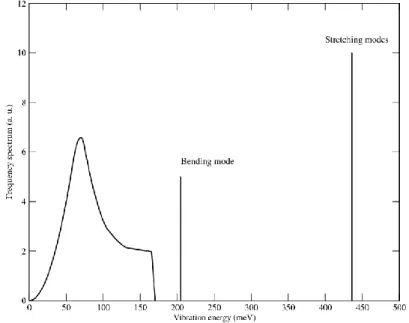
As an illustrative example, Figure 2.2 shows the frequency spectrum of 1_{H in H}

2O at 294 K of the

JEFF-3.1.1 nuclear data library [4]. The solid-type or continuous spectrum is seen for the lower vibration energies, while the internal modes of the water molecule are described by the two discrete energies. The first oscillator accounts for the bending mode and the second the stretching modes (symmetric and asymmetric).

Fig. 2.2 Continuous frequency spectra and intramolecular vibration modes of 1_{H H}

2O at 294 K for

JEFF-3.1.1 nuclear data library.

In the following subsections it will be analyzed how to calculate the scattering law due to each contribution of the partial spectra.

(33)

32

2.5.1 The phonon expansion

For the continuous frequency spectra we do an expansion in series of the time-dependent part of the exponential of eq. (45): 𝑒−𝛾𝑠(𝑡)_{= 𝑒}−𝛼𝜆𝑠_∑ 1 𝑛![𝛼 ∫ 𝜌(𝛽) 2𝛽𝑠𝑖𝑛ℎ(𝛽/2)𝑒 −𝛽/2_𝑒−𝑖𝛽𝑡_𝑑𝛽 ∞ −∞ ] 𝑛 , 𝑛 𝑛=0 (47)

where s is the Debye-Waller factor, given by:

𝜆𝑠= ∫ 𝜌(𝛽) 2𝛽𝑠𝑖𝑛ℎ(𝛽/2)𝑒 −𝛽/2_𝑑𝛽. ∞ −∞ (48)

So the scattering function for the solid-type spectrum:

𝑆𝑐(𝛼, 𝛽) = 𝑒−𝛼𝜆𝑠∑ 1 𝑛!𝛼 𝑛_𝑥 1 2𝜋∫ 𝑒 𝑖𝛽𝑡 ∞ −∞ [∫ 𝜌(𝛽′) 2𝛽′𝑠𝑖𝑛ℎ(𝛽′/2)𝑒 −𝛽′_/2 𝑒−𝑖𝛽′𝑡𝑑𝛽′ ∞ −∞ ] 𝑛 𝑑𝑡̂ 𝑛 𝑛=0 . (49)

Renaming the whole second factor of eq. (51) as 𝜆𝑆𝑛𝑇𝑛(𝛽):

𝑆𝑐(𝛼, 𝛽) = 𝑒−𝛼𝜆𝑠∑ 1 𝑛![𝛼𝜆𝑠] 𝑛_𝑇 𝑛(𝛽) 𝑛 𝑛=0 = 𝑒−𝛼𝜆𝑠_[𝑇 0(𝛽) + 𝛼𝜆𝑠𝑇1(𝛽) + 𝛼2𝜆𝑠2𝑇2(𝛽)] (50) 𝑇0(𝛽) = 1 2𝜋∫ 𝑒 𝑖𝛽𝑡_𝑑𝑡 ∞ −∞ = 𝛿(𝛽) (51) 𝑇1(𝛽) = ∫ 𝜌(𝛽) 2𝛽𝑠𝑖𝑛ℎ(𝛽/2)𝑒−𝛽 ′_/2 𝜆𝑠 [1 2𝜋∫ 𝑒 𝑖(𝛽−𝛽′)𝑡 ∞ −∞ ] 𝑑𝛽′ ∞ −∞ = 𝜌(𝛽) 2𝛽𝑠𝑖𝑛ℎ(𝛽/2)𝑒−𝛽/2 𝜆𝑠 (52)

In general the functions 𝑇𝑛(𝛽) are obtained recursively as:

𝑇𝑛(𝛽) = ∫ 𝑇1(𝛽′)𝑇𝑛−1(𝛽 − 𝛽′)𝑑𝛽′ ∞

−∞

, (53)

where the number of phonons exchanged n is given as input in LEAPR. Typically, 𝑛 = 200 is fair enough to converge the series.

As the function for 𝑛 = 0 is a delta function, this term is computed separately doing the convolution with the translational component, as we will see later. This term is called the zero-phonon term.

(34)

33

2.5.2 Molecular translations

In LEAPR the translation of the water molecules is modeled by a free gas law or by a diffusion model.

2.5.2.1 The free gas model

The first possibility is to model the translational part as a free gas distribution. Replacing eq. (42) in eq. (28) and performing a Fourier transform in time, we have an analytic expression for the translational scattering law: 𝑆𝑡(𝑞̅, 𝜔) = ( 𝛽 4𝜋𝐸𝑟 ) 1/2𝑒𝑥𝑝 (− 𝛽 4𝐸𝑟 [ℏ2_𝜔2_{− 2ℏ𝜔𝐸} 𝑟]), (54)

where 𝐸𝑟 is the recoil energy, given by:

𝐸𝑟 =

ℏ2_𝑞2

2𝑀 . (55) Changing variable in eq. (56) yields:

𝑆𝑡(𝛼, 𝛽) = 1 √4𝜋𝜔𝑡𝛼 𝑒𝑥𝑝 [−(𝜔𝑡+ 𝛽) 2 4𝜔𝑡𝛼 ] ; (𝛽 < 0) (56)

The eq. (58) is valid for the down-scattering regime (𝛽 > 0). The principle of detailed balance applies for 𝛽 > 0.

The combined scattering laws corresponding to the solid-type spectra 𝑆𝑐(𝛼, 𝛽) and the translational

mode 𝑆𝑡(𝛼, 𝛽) are obtained by doing the following convolution:

𝑆𝑐,𝑡(𝛼, 𝛽) = 𝑆𝑡(𝛼, 𝛽)𝑒−𝛼𝜆𝑠+ ∫ 𝑆𝑡(𝛼, 𝛽′)𝑆𝑠(𝛼, 𝛽 − 𝛽′)𝑑𝛽′ ∞

−∞

. (57)

As stated in the previous subsection, the zero-phonon term of the phonon expansion is convoluted with the translational mode, accounted in the first term of eq. (50).

2.5.2.2 The Egelstaff and Schofield diffusion model

Egelstaff and Schofield developed a diffusion model called “effective width model” [10]. The analytic expression for the frequency spectrum is:

𝜌𝑡(𝛽) = 𝜔𝑡

4𝑐

𝜋𝛽√𝑐2+ 1/4 𝑠𝑖𝑛ℎ(𝛽/2)𝐾1(𝛽√𝑐2+ 1/4), (58) where 𝐾1 is the modified Bessel function of second kind, 𝜔𝑡 is the translational weight and c is the

dimensionless diffusion constant. Both are provided as inputs in LEAPR. The parameter 𝑐 links the translational weight and the molecular diffusion coefficient 𝐷:

(35)

34 𝑐 =𝑀𝐻𝐷

𝜔𝑡ℏ

. (59)

Under this spectrum, the analytic form of the translational part of the scattering law is:

𝑆𝑡(𝛼, 𝛽) = 2𝑐𝜔𝑡𝛼 𝜋 𝑒𝑥𝑝[2𝑐 2_𝜔 𝑡𝛼 − 𝛽/2] √𝑐 + 1/4 √𝛽2_{+ 4𝑐}2_𝜔 𝑡2𝛼2 𝐾1(√𝑐 + 1/4√𝛽2+ 4𝑐2𝜔𝑡2𝛼2). (60)

2.5.3 The intramolecular vibration modes

The oscillators will model the internal vibration modes present in a polyatomic molecule. Their distribution is a delta function in an energy . If the sub-index 𝑖 describes each discrete oscillator, then the corresponding scattering law is given by:

𝑆𝑖(𝛼, 𝛽) = 𝑒−𝛼𝜆𝑖 ∑ [𝛿(𝛽 − 𝑛𝛽𝑖)𝐼𝑛( 𝛼𝜔𝑖 𝛽𝑖𝑠𝑖𝑛ℎ(𝛽𝑖/2) ) 𝑒−𝑛𝛽𝑖/2_] ∞ 𝑛=−∞ , (61) where 𝜆𝑖 = 𝜔𝑖 𝑐𝑜𝑡ℎ(𝛽𝑖/2) 𝛽𝑖

If there is only one discrete oscillator, then the convolution with the scattering laws of the rotational and translational modes is done in the following way:

𝑆(𝛼, 𝛽) = ∫ 𝑆1(𝛼, 𝛽′)𝑆𝑐,𝑡(𝛼, 𝛽 − 𝛽′)𝑑𝛽′ ∞

−∞

, (62)

where 𝑆1 is obtained with eq. (63) and 𝑆𝑐,𝑡 comes from eq. (59).

If there are two internal modes, then:

𝑆(𝛼, 𝛽) = ∫ 𝑆2(𝛼, 𝛽′)𝑆𝑠,𝑡,1(𝛼, 𝛽 − 𝛽′)𝑑𝛽′ ∞

−∞

, (63)

Improvement of the thermal and epithermal neutron scattering data for the interpretation of integral experiments

HAL Id: tel-01835720

https://tel.archives-ouvertes.fr/tel-01835720

Improvement of the thermal and epithermal neutron

scattering data for the interpretation of integral

experiments

Juan Scotta

To cite this version:

UNIVERSITE D’AIX-MARSEILLE

CEA Cadarache/ DEN / DER / SPRC / Laboratoire d’Etudes de Physiques

Thèse présentée pour obtenir le grade universitaire de docteur

Discipline : ED352 – PHYSIQUE ET SCIENCES DE LA MATIERE

Spécialité : Energie, Rayonnement et Plasma

Juan Pablo SCOTTA

Amélioration des données neutroniques de diffusion

thermique et epithermique pour l’interprétation des mesures

intégrales

Soutenue le 26/09/2017 devant le jury :

Luiz LEAL

IRSN

Examinateur

Cyrille DE SAINT JEAN

CEA Cadarache

Examinateur

Jose BUSTO

Université d’Aix Marseille

Examinateur

Florent REAL

Université de Lille

Rapporteur

Florencia CANTARGI

Centro Atomico Bariloche (ARG)

Rapporteur

Gilles NOGUERE

CEA Cadarache

Directeur de thèse

Abstract

Résumé

Contents

𝜇̅

𝜇̅

List of tables

List of figures

Chapter 1

Introduction

1.1 Context

1.2 Motivations

1.3 Objectives

1.4 Report description

Chapter 2

Thermal neutron scattering

2.1 Introduction to thermal neutron scattering theory

2.2 The coherent and incoherent cross sections

2.3 The coherent and incoherent scattering functions

2.4 The approximations of scattering in light water

2.4.1 The incoherent approximation

2.4.2 The Gaussian approximation

2.5 The evaluation of the scattering law with the LEAPR module of NJOY

2.5.1 The phonon expansion

2.5.2 Molecular translations

2.5.2.1 The free gas model

2.5.2.2 The Egelstaff and Schofield diffusion model

2.5.3 The intramolecular vibration modes