Maximum Entropy Production and Time Varying Problems: The Seasonal Cycle in a Conceptual Climate Model

HAL Id: hal-03209377

https://hal.archives-ouvertes.fr/hal-03209377

HAL is a multi-disciplinary open access archive for the deposit and dissemination of sci-entific research documents, whether they are pub-lished or not. The documents may come from teaching and research institutions in France or abroad, or from public or private research centers.

L’archive ouverte pluridisciplinaire HAL, est destinée au dépôt et à la diffusion de documents scientifiques de niveau recherche, publiés ou non, émanant des établissements d’enseignement et de recherche français ou étrangers, des laboratoires publics ou privés.

Problems: The Seasonal Cycle in a Conceptual Climate

Model

Didier Paillard, Corentin Herbert

To cite this version:

Didier Paillard, Corentin Herbert. Maximum Entropy Production and Time Varying Problems: The Seasonal Cycle in a Conceptual Climate Model. Entropy, MDPI, 2013, 15 (12), pp.2846-2860. �10.3390/e15072846�. �hal-03209377�

entropy

ISSN 1099-4300

www.mdpi.com/journal/entropy Article

Maximum Entropy Production and Time Varying Problems:

The Seasonal Cycle in a Conceptual Climate Model

Didier Paillard 1,_{* and Corentin Herbert} 1,2

1 _{Laboratoire des Sciences du Climat et de l'Environnement, IPSL, Orme des Merisiers,}

Gif-sur-Yvette 91191, France

2 _{National Center for Atmospheric Research, P.O. Box 3000, Boulder, CO 80307, USA;}

E-Mail: cherbert@ucar.edu

* Author to whom correspondence should be addressed; E-Mail: didier.paillard@lsce.ipsl.fr.

Received: 26 April 2013; in revised form: 5 July 2013 / Accepted: 17 July 2013 / Published: 19 July 2013

Abstract: It has been suggested that the maximum entropy production (MEP) principle, or

MEP hypothesis, could be an interesting tool to compute climatic variables like temperature. In this climatological context, a major limitation of MEP is that it is generally assumed to be applicable only for stationary systems. It is therefore often anticipated that critical climatic features like the seasonal cycle or climatic change cannot be represented within this framework. We discuss here several possibilities in order to introduce time- varying climatic problems using the MEP formalism. We will show that it is possible to formulate a MEP model which accounts for time evolution in a consistent way. This formulation leads to physically relevant results as long as the internal time scales associated with thermal inertia are small compared to the speed of external changes. We will focus on transient changes as well as on the seasonal cycle in a conceptual climate box-model in order to discuss the physical relevance of such an extension of the MEP framework.

Keywords: maximum entropy; maximum entropy production; non-equilibrium;

climate modeling

1. Introduction

Several decades ago, Paltridge [1] suggested that the stationary state of the climate system could be computed through a simple variational principle. An objective or cost function to be optimized was

found empirically. This function was later recognized [2] to be the production of thermodynamical entropy due to atmospheric and oceanic heat transfers. These results were received with a lot of skepticism in the climate community, since there is no widely accepted fundamental physical reason for maximizing entropy production, even though such a MEP principle had been proposed by some scientists at about the same time [3]. Besides, the Paltridge model is purely thermodynamical and its results do not depend on important dynamical effects such as Earth’s rotation rate for instance. The original model has some empirical parameters in its radiative formulas: there was some possibility that the remarkable agreement between model results and observations did partly result from the choices of radiative parameters. The model was mostly seen as a curiosity, and only very few people tried to use or analyse it. A nice reformulation of the model with a quasi-analytic solution was given by O’Brien [4].

In recent years, there has been renewed interest in this type of model. It was suggested that the MEP principle could be useful in climate models [5] and new efforts were aimed at justifying this idea [6–8]. Still, there is yet no consensus on the applicability of the MEP hypothesis to physics in general [9] and to climate modeling in particular [10,11]. Quite possibly, when or if applicable, the MEP hypothesis might be only a thermodynamical, or coarse-grained approximation of a more complex dynamical reality, whose usefulness depends of the problem considered [12]. In this context, it appears nevertheless interesting to investigate how well such a model performs and how far it can be developed. In this direction, we have shown earlier [13] that it is possible to formulate a MEP climate model with a radiative code based on standard atmospheric formulations, without adjustable parameters, at the cost of ignoring the effect of clouds. Though systematically biased towards higher temperatures by about 8 °C, this “clear-sky” model is quite successful in reproducing, in annual mean, the meridional energy transport and the large scale temperature gradients, but also the climate sensitivity to albedo changes when compared with a state-of-the-art general circulation model. This highlights that the successful results of Paltridge’s model are probably not fortuitous.

A potential difficulty of using the MEP hypothesis in a climate model is the necessity to formulate a stationary problem. Indeed, it is not clear a priori that such a variational principle can accomodate a time-dependent question. The climate system is characterized by a strong seasonal cycle and a model which predicts only annual mean values, like the current MEP ones, is therefore not very relevant for most climatic questions. An interesting extension would be therefore to allow for time-varying problems within the MEP formulation. It is beyond the scope of this paper to discuss the physical validity or the applicability of the MEP principle to generic or even specific physical problems. We will restrict ourself to the presentation and discussion of several conceptual ideas for such a MEP climate model that accounts for time-variations, in particular with the goal to reproduce a meaningful seasonal cycle. This first example could be used as a basis for further developments, both theoretical and applied, concerning MEP principles.

2. Formulation of a MEP Climate Model

2.1. The Annual Mean Stationary Model

First, we will formulate our MEP climate model in its annual mean version. We are interested in

computing the temperature Ti at each point i, where i = 1 to N (N being the number of “points” or

“boxes” in the spatial domain of interest). A generic model layout is given on Figure 1.

Figure 1. A generic climate model consists of boxes with temperatures Ti exchanging

radiative fluxes rik and rki with space and boxes on the same vertical column, and turbulent

heat fluxes Fji with neighbouring boxes. This can be summarized in a net radiative input

Ri(Tk) = ∑k(rki − rik) and the non-radiative heat convergence γi = ∑j Fji.

The local heat conservation can be written as follows: ( ) i i i k i dT c R T dt    (1)

where Ri(Tk) corresponds to the net radiative balance of box i (in W), given as an explicit function of

temperatures (Ti, but also the temperatures Tk of boxes which exchange radiatively with box i, i.e.,

boxes in the same vertical column), ci are the heat capacities of each box (J.K−1), and γi are the heat

convergences due to atmospheric fluxes. The MEP principle states that, in the stationarity situation

(i.e., when dTi/dt = 0) the entropy production associated with γi should be maximum, under the

constraint of global energy conservation. Indeed, the convergences γi are “internal” to the system and

must sum up to zero. In other words, according to the MEP hypothesis, the solution of the problem is a stationary point of the Lagrange function:











where β is the Lagrange multiplier associated with global energy conservation. The right term is

obtained by using Equation (1) in its stationary version, i.e., γi = −Ri(Tk). Note that β is an inverse

We will see below in simplified cases, that Tg is indeed some global “averaged” temperature. The

variational problem in Equation (2) can be solved formally as follows:

0 2 ( ) 1 0 k i k i i k i L R R T T T T T   _         _{ }  _   





For a given value of β, we can in principle solve the system of N Equations (3) in the variables Ti

thus giving a solution Ti(β). Though typically non-linear, this system appears well-behaved in cases of

interest. The matrix (∂Rk/∂Ti) is sparse since the radiative fluxes Ri will depend on the temperatures of

the same vertical column only, but not on other neighbouring points. The Equation (4) can be expressed as a function of β only, which therefore gives a solution.

The only inputs of such a model are a discretization of the domain of interest, and the

radiative functions Ri(T). The model is purely thermodynamical and there is no need to use a

“spatially structured” discretization since there is at this stage no vector calculus at all: the boxes do not need to be on a structured grid. If we restrict ourselves to a “clear sky” situation and neglect the

effect of clouds, the radiative functions Ri(T) can be computed from standard formulations, assuming

prescribed levels of greenhouse gases in the atmosphere (H2O, CO2, O3), as well as a given surface albedo. This model was studied in Herbert et al. [13] on a 72 × 96 horizontal regular grid with a surface level and one atmospheric level, and also for many levels in a vertical temperature profile [14]. 2.2. A Simplified Version of the Previous Model

In order to introduce time variations or the annual cycle, it is interesting to formulate a simplified version of the model described above, that can be easily solved analytically. We will make here the

hypothesis that the radiative functions Ri(T) are not only linear in T (which is a relatively mild

hypothesis, since the true radiative functions are smooth functions of T with the dominant contribution

being of the form σT4, and therefore can be linearized at least in a neighborhood of the solution of the

problem); but also that Ri(T) are local, i.e., depend only on the box temperature Ti: Ri = Ri(Ti). This

last hypothesis is certainly not valid for a vertical atmospheric temperature profile, but it allows for quite nice simplifications of the above equations, and therefore for much better insights into the generic problem.

We therefore have Ri = bi (T0i − Ti) where T0i is the temperature that box i would have in the

absence of any non-radiative exchange with other boxes, i.e., if γi = 0. We can therefore call it the

“radiative temperature” of box i. Note also that the coefficients bi are extensive quantities (in W.K−1)

locally proportional to the size (area or volume) of box i. With this drastic simplification, the above problem leads to the following simple solution:

0i i T T   ₍₅₎

2 0 0 1 _i i i g _i i i b T T bT   _ _  





In other words, the global inverse temperature β is some kind of weighted averaged of the radiative

temperatures T0i using the (extensive) coefficients bi as weights, while the local temperatures Ti are the

geometric means between the local radiative temperature T0i and the global temperature Tg. It appears

here quite obvious and natural that the solution is unique and bears some simple physical signification. 2.3. A Two-Box Example

In order to illustrate the above MEP solutions, we will present results in the simplest possible situation. Let’s assume that the Earth climate can be represented by only two boxes, a tropical one and a polar one, as represented in Figure 2.

Figure 2. A simple case with a two-box model.

The stationary MEP principle can be easily illustrated here. The local energy conservation in Equation (1) gives Q = F12 = γ2 = − γ1, which leads to T1 = T01 − Q/b and T2 = T02 + Q/b. The unknown or implicit meridional flux Q is obtained through the maximisation of the entropy production σ = γ1/T1 + γ2/T2 as shown in Figure 3.

Figure 3. The entropy production σ = γ1/T1 + γ2/T2 = b x [(T02 + x)−1 − (T01 − x)−1] as a function of the heat flux x = Q/b. Here T01 = 300 K and T02 = 280 K. It is quite clear that this function has a unique positive maximum between the two roots obtained for Q = x = 0 (purely radiative case) and for the isothermal situation x = (T01 − T02)/2. This maximum is given by Equations (5) and (6).

This equilibrium situation has been already described and discussed in numerous papers, both for theoretical cases, but also for the climate of several planets in the solar system [15,16]. In this paper we will focus on the time varying problem.

3. A Time-Dependent MEP Formulation with Integrated Entropy Production

The natural and simplest possible extension of the MEP hypothesis to a time varying problem is to maximize the entropy production integrated over time. This turns out to be rather straightforward as illustrated below.

3.1. The Model Equations

In order to write a time dependent version of Equations (3) and (4), we need to relax the stationarity

assumption. In fact, in the general case, we can substitute the γi from Equation (1) in order to obtain a

new Lagrange function:



















where all variables are now functions of time. The summation is now over space (discrete index i) and over time (continuous variable t). Though not in the context of seasonal variations, a rather similar formulation was suggested earlier [17] where the maximisation of entropy production was performed at each time step in a simple model, in order to investigate the notion of dynamical stability of the MEP equilibrium. It should be emphasized that β = β(t) must depend of time, since the heat

convergences γi should sum up to zero at all time. In other words, the “heat transports through time”

are explicitly and solely given by ci dTi/dt while “through space” we have both explicit heat fluxes

associated with Ri(Tk) and implicit ones with γi. The Lagrange function is now a functional of both Ti

and its time derivative T'i = dTi/dt. This new variational problem is well-known in classical mechanics,

and the solution is given by the Euler-Lagrange equations. This leads to:

2 ( ) 1 0 k i i k i i i k i R R T L d L c T dt T T T T    _{ }            _{ }  _{ }  _    





with β' = dβ/dt. These equations are very similar to Equations (3) and (4) and formally their resolution is similar. For a given function β(t), we can obtain its time-derivative β'(t) and we thus can solve

system Equation (8) to obtain the temperatures Ti(t) at each point i. After substitution in Equation (9)

we obtain a differential equation in β(t), β'(t) and β"(t), whose resolution solves the problem. In order to get some insight into this solution, we will use the above linear approximation for the radiative functions. We will also assume that the system under consideration is homogeneous, in the sense that

the ratio ci/bi is here a fixed constant a. Note that a is a time which represents the thermal inertia of the

0 0 i i i T T T a        (10)

where α = α(t) is the inverse square root of β(t) − a β'(t). After substitution into Equation (9) we get a simple linear differential equation for α(t), whose solution will therefore solve the problem:

















where T'0i is the time derivative of T0i. Note that Equations (10) and (11) are quite similar to their stationary equivalents in Equations (5) and (6).

There are two time scales in this equation. The first time scale is given by 1/τ~T'0i/T0i, i.e., the speed of external changes. The second one is the constant a which reflect the thermal inertia of the medium.

In particular, when the heat capacities ci, and therefore the constant a, are vanishingly small, we obtain

a “quasi-stationary” solution: we get the exact same formula as in Equations (5) and (6), though here the temperatures T0i(t) are assumed to depend on time. This is equivalent to the “quasi-static” approximation used in classical thermodynamics.

We can also consider the opposite situation with the thermal inertia a being extremely large. In this case, Equation (11) becomes:

0 0 0 1 2 i i i i i i i T b T b T  _  _       _{ }  





In other words, the temperatures will readjust rapidly to the changing forcing T0i(t) through the

global function α∞(t) given by Equation (12), even if the heat capacities are infinite. This does not

seem physically very relevant, and we are here probably outside the validity range of the MEP hypothesis. As we will see below, this adjustment may be interpreted in terms of (potentially unrealistically) large “implicit heat fluxes” that will enforce a maximum entropy production. This is illustrated in the following example.

3.2. The Two-Box Case with a Step Change

As a proof of concept for time varying problems, we will first discuss the two-box situation when submitted to a step-like change at some given time t = 0. This will allow for a much simpler discussion of the physical relevance of the model. To avoid discontinuities, we will use an hyperbolic tangent to represent a change that will occur over a characteristic time τ:

01 01 01 01 02 02 02 02 1 tanh( / ) 1 tanh( / ) ( ) ( ) ( ) ( ) 2 2 S E S t S E S t T t T  T T _   _ T t T  T T _   _     (13)

The model will jump from one equilibrium {T1S,T2S} at the start (for large negative times) to a new

one {T1E,T2E} at the end (for large positive times), as given in the previous section, with a transition

near time t = 0 obtained by solving Equation (11), thus giving the time evolution {T1(t),T2(t)}. As discussed above, we might also be interested in the limit case a = 0 (“quasi-stationary” or “quasi-static”

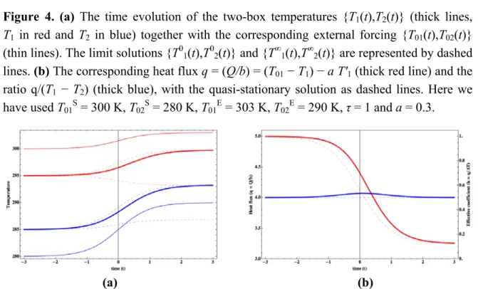
Figure 4 below is presenting the results obtained for a smaller than τ. We see that the computed solution behaves as expected, jumping from one equilibrium to the other, with a time delay of order a

when compared to the “quasi-static” solution {T01(t),T02(t)}. The implicit heat flux Q between the two

boxes also behaves as expected, changing from large values when the temperature gradient is large at the beginning, to smaller ones when the gradient is reduced. It is worth emphasizing that, in contrast to

traditional models, there is here no a priori link between Q and the temperature gradient (T1 − T2). It is

possible to define a posteriori a heat exchange coefficient k as k = Q/(T1 − T2). In traditional models,

this ratio is severely constrained by some dynamical processes or even fixed. Here, its time evolution can therefore be used to track possible inconsistencies. In Figure 4b, changes in k are rather smooth and small. In the quasi-stationary case (dotted blue line), changes in k are vanishingly small (they are second order in ∆T/T).

Figure 4. (a) The time evolution of the two-box temperatures {T1(t),T2(t)} (thick lines, T1 in red and T2 in blue) together with the corresponding external forcing {T01(t),T02(t)}

(thin lines). The limit solutions {T01(t),T02(t)} and {T∞1(t),T∞2(t)} are represented by dashed

lines. (b) The corresponding heat flux q = (Q/b) = (T01 − T1) − a T'1 (thick red line) and the

ratio q/(T1 − T2) (thick blue), with the quasi-stationary solution as dashed lines. Here we

have used T01S = 300 K, T02S = 280 K, T01E = 303 K, T02E = 290 K, τ = 1 and a = 0.3.

(a) (b)

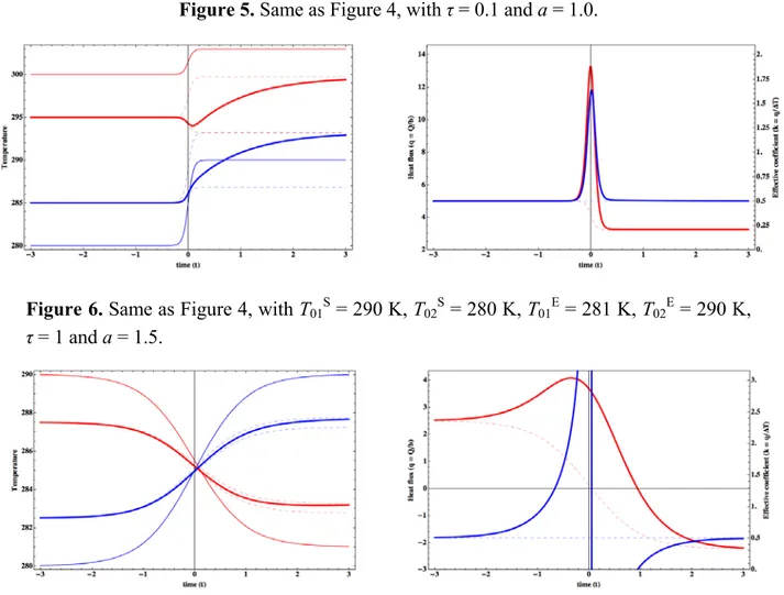
A rather different behaviour is observed in Figure 5, when the transition is much more abrupt. Here the solution T1(t) first decreases, which is physically quite unexpected since both external forcings

correspond to warming. In fact T1(t) is first following the T∞1(t) limit solution before converging

slowly towards the equilibrium T1E. The corresponding heat flux shows a very large transient

associated with the rapid change in the forcing, that cannot be absorbed by the heat reservoirs due to the large heat capacities. Accordingly, changes in k are also very large and abrupt.

But an even more interesting behaviour is obtained in Figure 6. Here, we are in a quasi-symmetrical situation, with the warm box being cooled, and the cold box being warmed by approximately the same amount. Even when using a very large thermal inertia a, we observe that there is almost no time lag between the external forcing T0i(t) and the model response. In fact, independently of the thermal

inertia, the two limit solutions T0i(t) and T∞i(t) become very close. In case of perfect symmetry, the

difference simply vanishes. Indeed, in this case, it can be seen in Equation (12) that the solution α∞(t)

is a constant. This implies that the global inverse temperature β(t) is also a constant, and in fact the

change, whatever the internal thermal inertial time scales. Again, this is obviously not quite physically relevant. Interestingly, the effect of thermal inertia is fully transfered to the implicit heat flux Q, and the effective coefficient k diverges and becomes negative, as shown on Figure 6b.

Figure 5. Same as Figure 4, with τ = 0.1 and a = 1.0.

Figure 6. Same as Figure 4, with T01S = 290 K, T02S = 280 K, T01E = 281 K, T02E = 290 K, τ = 1 and a = 1.5.

It should be emphasized that, within the MEP principle, there is no a priori reason to constrain k in any way. For instance, in a meteorological context it is possible to transport heat “uphill” from cold to warmer regions, through latent heat or mechanical energy transports. The MEP principle suggests that such apparent local or temporary violations of the Second Law are favoured when the corresponding global entropy production is increased. But obviously, it is necessary to discuss the physical relevance of such cases. The alternative is to enforce additional constraints (e.g., positivity of k): this is also quite straightforward in the MEP context as we will show later.

3.3. The Two-Box Case with a Seasonal Cycle

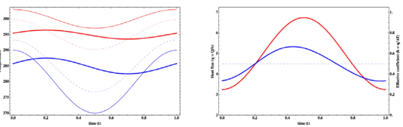
Our initial motivation is linked to the representation of the seasonal cycle in a MEP climate model. In this case, the forcing time scale is one year, whereas the largest thermal inertia is associated with ocean mixed layer, with a typical value of a of the order of about two weeks to a month. A priori, we are here in the situation where inertial time scales are smaller than the forcing changes. This is indeed the case in Figure 7 where we have used a simple sinusoidal forcing given by (in Kelvin):

01( ) 01 01cos(2 02) ( ) 02 02cos(2 )

As expected, the resulting temperatures {T1(t),T2(t)} lag the forcing with a time scale of order a. The amplitude of the response is slightly smaller than in the quasi-stationary case (i.e., without thermal inertia), as expected from a damped response. As before, there is a consistent, though non constant,

relationship between the heat flux Q and the temperature gradient (T1 − T2), with a larger flux when the

gradient is larger.

Figure 7. (a) The time evolution of the two-box temperatures {T1(t),T2(t)} (thick lines, T1 in red and T2 in blue) together with the corresponding external forcing {T01(t),T02(t)} (thin lines) and the quasi-stationary solution (dashed lines). T01 = 300 K, ∆T01 = 3 K, T02 = 280 K, ∆T02 = 10 K; (b) The corresponding heat flux q = (Q/b) = (T01 − T1) − a T'1

(thick red line) and the ratio q/(T1 − T2) (thick blue), with the quasi-stationary solution as

dashed lines. Here we have used a = 0.1.

(a) (b)

When the thermal inertia is larger, as illustrated in Figure 8, for a = 0.5, i.e., when the thermal inertia time constant is equal to half the periodicity of the forcing, we observe that the lags are very different in the cold box and in the warm one. Again, this appears to be a quite non-physical result.

We note also that the induced heat flux Q and therefore also the ratio Q/(T1 − T2) become negative

during the cycle, with heat flowing from the cold reservoir towards the warm one.

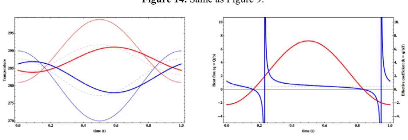
But again, the most interesting situation is the almost symmetrical one shown in Figure 9. As in the step-like situation, there is no more lag between forcing and response. This is again due to an

almost constant “global temperature” Tg = 1/β. The rather large thermal inertia leads to quite

unrealistic heat fluxes.

Figure 9. Same as Figure 7, with T01 = 290 K, ∆T01 = −9 K, T02 = 280 K, ∆T02 = 10 K, a = 0.5.

4. A Relaxation Formulation

Seasonal climatic variations are almost symmetrical with respect to the equator. Obviously, the above formulation is unlikely to provide reasonable results for a seasonal MEP climate model. We therefore need to investigate other possible formulations in order to build such a model. The root of the difficulty identified on the above examples (again, beyond the lack of any well-established physical justification) is linked to the reduction of the dimensionality of the problem. Indeed, the simple MEP formulation outlined above, though quite appealing, reduces a N-dimensional dynamical

system to a 1-dimensional one that involves only one “global temperature” Tg, with all other

temperatures being unequivocally linked to it. In the symmetrical 2-box cases, this unique degree of freedom is constant by symmetry, and the thermal inertia does not appear in local temperatures, but only in implicit fluxes.In fact, any global variational formulation of the problem is likely to lead to the same problem.

It seems therefore important to keep as many degrees of freedom as in the original problem, that is a N-dimensional dynamical system. If Equation (1) is to be used, we need to specify how to compute the implicit convergences γi as functions of the forcing or state variables. The easiest way to write a consistent MEP closure of this problem is to assume a relaxation to the MEP quasi-stationary solution:

0 ( ) i i i k i dT c R T dt    (15)

where γi0 is the heat convergence associated with the quasi-stationary solution T0i. This set of equations

for the energy conservation can equivalently be written as:

0 ( ) ( ) i i i k i k dT c R T R T dt   (16)

As in the previous case, this formulation is likely to be valid for vanishingly small heat capacities ci.

But now each temperature Ti is a dynamical variable with its own evolution, not necessarily linked to

integrated entropy production functional, i.e., a stationary point of the Lagrange functional L(Ti,T'i,β)

written in Equation (7). But the heat fluxes are still obtained by assuming that they are constantly driving the temperatures towards the instantaneous MEP state, though each temperature has its own inertia associated with local heat capacities, or any other deterministic process. In fact, this is somewhat reminiscent of systems close to equilibrium, for which thermodynamical fluxes will tend to relax the system towards the maximum entropy state. In the following, we apply this new formulation to the two-box model studied before.

4.1. The Two-Box Case with a Step Change

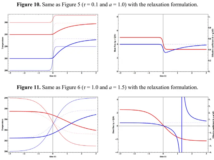
As expected, the results are very similar to the ones obtained by the previous method when the internal time scale a is smaller than the external one τ, since this situation is close to the quasi-stationary one. For a rapid external change, we obtain results show in Figure 10, to be contrasted with results in Figure 5. By construction, we do not get the previous non-physical result of a decreasing temperature T1(t) during the transition. Furthermore, the variations in the implicit heat flux Q as well as the effective coefficient k are much smaller than before. This second formulation behaves therefore much more consistently than the first one.

Figure 10. Same as Figure 5 (τ = 0.1 and a = 1.0) with the relaxation formulation.

Figure 11. Same as Figure 6 (τ = 1.0 and a = 1.5) with the relaxation formulation.

In case of the almost symmetrical forcing, we now also have a physically consistent lag between the forcing and the model response, as shown in Figure 11. It should be noted that the implicit heat flux Q is now chosen to be equal to its quasi-stationary value. Compared to Figure 6, its changes are now monotonous. But, as before, it does not change in accordance with the temperature difference

T2(t) − T1(t), hence a widly varying effective coefficient k that becomes negative, i.e., with a heat flux from the cold box to the warm one, in contradiction with the Second Law. It is of course quite easy to constrain the heat flux to flow in the direction of the temperature gradient, which gives the solution shown in Figure 12.

Figure 12. Same as Figure 11 with k constrained to be positive.

4.2. The Two-Box Case with a Seasonal Cycle

When applying a periodic forcing, in the case of a large thermal inertia, we obtain the results shown in Figure 13, that should be compared to Figure 8. Now the lags between forcing and response are similar in both boxes, by construction. Though they still vary quite significantly, the heat flux Q and the corresponding effective coefficient k are now well-behaved.

Figure 13. Similarity to Figure 8 (a = 0.5).

When applying a symmetrical forcing, we obtain the results shown of Figure 14, that should be compared to Figure 9. Again, in this formulation, we now recover physically relevant lags between forcing and response. As above, the heat flux Q may flow from the cold box to the warm one, in contradiction with the Second Law something which could easily be corrected by applying the proper additional constraint as for Figure 11.

Figure 14. Same as Figure 9.

5. Conclusions

We have extended a simple MEP model to time-varying problems, beyond the classical “quasi-stationary” or “quasi-static” cases. We have shown that the formulation of such an extended MEP model might lead to non-physical situations in our case study, and that a relaxation formulation is more likely to provide physically consistent results than a simple straightforward application of the MEP principle. This is particularly true when the internal inertial time scales are comparable to or larger than the rate of the external changes, in which cases the internal dynamics needs to be more explicitly represented. The formulations presented here can be easily adapted to accommodate for additional constraints on the dynamics, for instance with the requirement that heat fluxes should flow in the direction of the temperature gradients (i.e., k > 0).

Our goal was to define a framework for representing a seasonal cycle in a MEP climate model. The relaxation formulation outlined in this paper appears to be a reasonable basis in this direction. The thermal time scale of the ocean mixed layer being of the order of two weeks over the continents, to about one or two months above the oceans [18], we will remain close to a quasi-stationary situation. Such a seasonally varying MEP climate model should therefore provide reasonable results without any assumption on the dynamics of the system, somewhat similarly to the annual averaged model first presented by Paltridge [1].

Acknowledgements

The authors would like to thank the two anonymous reviewers whose comments help to clarify the manuscript. The National Center for Atmospheric Research is sponsored by the National Science Foundation.

Conflict of Interest

The authors declare no conflict of interest.

References

1. Paltridge, G. Global dynamics and climate—A system of minimum entropy exchange. Q. J. Roy. Meteorol. Soc. 1975, 101, 475–484.

2. Paltridge, G. The steady-state format of global climate. Q. J. Roy. Meteorol. Soc. 1978, 104, 927–945. 3. Ziegler, H. An Introduction to Thermomechanics; North-Holland: Amsterdam, The Netherlands, 1983. 4. O’Brien, D.; Stephens, G. Entropy and climate. II: Simple models. Q. J. Roy. Meteorol. Soc.

1995, 121, 1773–1796.

5. Kleidon, A. Nonequilibrium thermodynamics and maximum entropy production in the Earth system. Naturwissenschaften 2009, 96, 653–677.

6. Dewar, R. Information theory explanation of the fluctuation theorem, maximum entropy production and self-organized criticality in non-equilibrium stationary states. J. Phys. A: Math. Theory 2003, 36, 631–641.

7. Martyushev, L.M.; Seleznev, V.D. Maximum entropy production principle in physics, chemistry and biology. Phys. Rep. 2006, 426, 1–45.

8. Jupp, T.E.; Cox, P.M. MEP and planetary climates: Insights from a two-box model containing atmospheric dynamics. Phil. Trans. R. Soc. B 2010, 365, 1355–1365.

9. Bruers, S. A discussion on maximum entropy production and information theory. J. Phys. A: Math. Theory 2007, 40, 7441–7450.

10. Pascale, S.; Gregory, J.M.; Ambaum, M.H.P.; Tailleux, R.; Lucarini, V. Vertical and horizontal processes in the global atmosphere and the maximum entropy production conjecture. Earth Syst. Dyn.

2012, 3, 19–32.

11. Goody, R. Maximum entropy production in climate theory. J. Atmos. Sci. 2007, 64, 2735–2739. 12. Dewar, R. Maximum entropy production as an inference algorithm that translates physical

assumptions into macroscopic predictions: Don’t shoot the messenger. Entropy 2009, 11, 931–944. 13. Herbert, C.; Paillard, D.; Kageyama, M.; Dubr+ulle, B. Present and Last Glacial Maximum

climates as states of maximum entropy production. Q. J. Roy. Meteorol. Soc. 2011, 137, 1059–1069. 14. Herbert, C.; Paillard, D.; Dubrulle, B. Vertical temperature profiles at maximum entropy

production with a net exchange radiative formulation. J. Clim. 2013, in press.

15. Lorenz, R.D.; Lunine, J.I.; Withers, P.G.; McKay, C.P. Titan, mars and earth: Entropy production by latitudinal heat transport. Geophys. Res. Lett. 2001, 28, 415–418.

16. Lorenz, R. The two-box model of climate: Limitations and applications to planetary habitability and maximum entropy production studies. Phil. Trans. R. Soc. B 2010, 365, 1349–1354.

17. Herbert, C.; Paillard, D.; Dubrulle, B. Entropy production and multiple equilibria: The case of the ice-albedo feedback. Earth Syst. Dyn. 2011, 2, 13–23.

18. Stine, A.R.; Huybers, P.; Fung, I.Y. Changes in the phase of the annual cycle of surface temperature. Nature 2009, 457, 435–440.

© 2013 by the authors; licensee MDPI, Basel, Switzerland. This article is an open access article distributed under the terms and conditions of the Creative Commons Attribution license (http://creativecommons.org/licenses/by/3.0/).