Multiscale Analysis of Intensive Longitudinal Biomedical Signals and its Clinical Applications

HAL Id: hal-01518074

https://hal.archives-ouvertes.fr/hal-01518074

Submitted on 4 May 2017

HAL is a multi-disciplinary open access archive for the deposit and dissemination of sci-entific research documents, whether they are pub-lished or not. The documents may come from teaching and research institutions in France or abroad, or from public or private research centers.

L’archive ouverte pluridisciplinaire HAL, est destinée au dépôt et à la diffusion de documents scientifiques de niveau recherche, publiés ou non, émanant des établissements d’enseignement et de recherche français ou étrangers, des laboratoires publics ou privés.

Multiscale Analysis of Intensive Longitudinal Biomedical

Signals and its Clinical Applications

Toru Nakamura, Ken Kiyono, Herwig Wendt, Patrice Abry, Yoshiharu

Yamamoto

To cite this version:

Toru Nakamura, Ken Kiyono, Herwig Wendt, Patrice Abry, Yoshiharu Yamamoto. Multiscale

Anal-ysis of Intensive Longitudinal Biomedical Signals and its Clinical Applications. Proceedings of

the IEEE, Institute of Electrical and Electronics Engineers, 2016, vol. 104 (n° 2), pp. 242-261. �10.1109/JPROC.2015.2491979�. �hal-01518074�

To link to this article : DOI :

10.1109/JPROC.2015.2491979

URL :

http://dx.doi.org/10.1109/JPROC.2015.2491979

To cite this version :

Nakamura, Toru and Kiyono, Ken and Wendt, Herwig

and Abry, Patrice and Yamamoto, Yoshiharu Multiscale Analysis of Intensive

Longitudinal Biomedical Signals and its Clinical Applications. (2016)

Proceedings of the IEEE, vol. 104 (n° 2). pp. 242-261. ISSN 0018-9219

O

pen

A

rchive

T

OULOUSE

A

rchive

O

uverte (

OATAO

)

OATAO is an open access repository that collects the work of Toulouse researchers and

makes it freely available over the web where possible.

This is an author-deposited version published in :

http://oatao.univ-toulouse.fr/

Eprints ID : 17027

Any correspondence concerning this service should be sent to the repository

administrator:

staff-oatao@listes-diff.inp-toulouse.fr

Multiscale Analysis of Intensive

Longitudinal Biomedical

Signals and Its Clinical

Applications

Recent advances in wearable and/or biomedical sensing technologies have made it

possible to record continuous biomedical signals over long periods of time. This

paper reviews multiscale approaches for their analysis.

By Toru Nakamura, Ken Kiyono, Herwig Wendt, Patrice Abry,

, and

Yoshiharu Yamamoto

ABSTRACT|_{Recent advances in wearable and/or biomedical} sensing technologies have made it possible to record very long-term, continuous biomedical signals, referred to as bio-medical intensive longitudinal data (ILD). To link ILD to clini-cal applications, such as personalized healthcare and disease prevention, the development of robust and reliable data anal-ysis techniques is considered important. In this review, we in-troduce multiscale analysis methods for and the applications to two types of intensive longitudinal biomedical signals, heart rate variability (HRV) and spontaneous physical activity (SPA) time series. It has been shown that these ILD have ro-bust characteristics unique to various multiscale complex sys-tems, and some parameters characterizing the multiscale complexity are in fact altered in pathological states, showing potential usability as a new type of ambient diagnostic and/ or prognostic tools. For example, parameters characterizing increased intermittency of HRV are found to be potentially

useful in detecting abnormality in the state of the autonomic nervous system, in particular the sympathetic hyperactivity, and intermittency parameters of SPA might also be useful in evaluating symptoms of psychiatric patients with depressive as well as manic episodes, all in the daily settings. Therefore, multiscale analysis might be a useful tool to extract informa-tion on clinical events occurring at multiple time scales dur-ing daily life and the underlydur-ing physiological control mechanisms from biomedical ILD.

KEYWORDS|_{Autonomic nervous system; complex biosignals;} dynamical disease; heart failure; heart rate variability; multi-scale fluctuations; psychiatric disorder; spontaneous physical activity

I . I N TR O D U CT I ON

Ambulatory assessments have recently started to become rapidly pervasive on a global scale. The development of such technologies allows us to obtain large-scale data by longitudinal recording of biomedical signals, such as heart rate and physical activity time series. For instance, in the last few years, a number of wearable devices and cloud services using them for healthcare management have been released at low cost [5]–[7]. However, methods to analyze this kind of data collected continu-ously in daily life, or so-called intensive longitudinal data (ILD) [9], have not yet been fully established. To gain useful information for better healthcare uses, it is impor-tant to characterize signal features related to underlying

(Corresponding author: Y. Yamamoto.)

T. Nakamura and Y. Yamamoto are with the Graduate School of Education, The University of Tokyo, Tokyo 113-0033, Japan (e-mail: yamamoto@p.u-tokyo.ac.jp). K. Kiyono is with the Graduate School of Engineering Science, Osaka University, Osaka 560-8531, Japan.

H. Wendt is with CNRS at IRIT, University of Toulouse, 3100 Toulouse, France. P. Abry is with CNRS at ENS de Lyon, Physics Department, 69007 Lyon, France.

physiological control mechanisms and clinical events oc-curring on multiple time scales.

In this review, we introduce studies on statistical and dynamical characterizations of signals called heart rate variability (HRV) [13], a sequence of heart inter-beat in-tervals measured by ambulatory electrocardiography, and spontaneous physical activity (SPA), or sometimes called locomotor activity, measured by acceleration sensors built, for instance, into a wrist band/watch [14], [15]. Be-cause the data collection for these signals is one of the easiest modes of ambulatory monitoring, these data are indeed two typical examples of ILD [9] that can be ob-tained from time scales of seconds, minutes, hours, and even days (or months in the case of SPA). These types of data contain signal components due to changes in physio-logical states and/or behavioral episodes (exercise, sleep, eating, etc.) in daily life. In addition to these limited

number of within-day states and/or episodes, they also

contain an even greater amount of fluctuations around changes in local means, known to show characteristics unique to various multiscale complex systems. These characteristics include long-range correlation [16], [17], fractality [18]–[21], multifractality [22], non-Gaussian [17], [23] and/or non-Poissonian [1], [2] behavior, and intermittency [3], [4], [11], [23]–[25].

From a biomedical perspective, the massive existence of signal components exhibiting such multiscale com-plexity is considered important for two reasons. First, as it is difficult for an individual to control her/his physio-logical states and behavioral episodes over a number of multiple time scales at the same time for a long period of recording during daily life, these components are most likely to be generated unconsciously without being af-fected much by the specific life-styles of patients. Thus, they are considered to provide robust measures reflecting intrinsic characteristics of underlying physiological con-trol mechanisms [26]. Notwithstanding this, these mea-sures for multiscale complexity have been shown to be altered in pathological states: e.g., myocardial infarction [27], [28] and heart failure [11], [23]–[25], [29] for HRV, and major depressive disorder [1], [2], [30] and schizophrenia [31] for SPA. Second, and more intrigu-ingly, it may be possible that statistical as well as dynam-ical features of these components (fluctuations) could provide information about early signs of abrupt changes in the state of the system [32], and in this case health and medical status.

The importance of studying statistical and dynamical features of fluctuations can be understood by using a schematic view of the dynamics of physiological regula-tions and the transition to a “dynamical disease” [33], [34] state [Fig. 1]. Traditionally, physiological regulations have been explained using the concept of homeostasis

(i.e., stability through constancy), maintaining constancy of a vital variable by sensing its deviation from a set point and providing feedback to correct the error. Short-range

negative correlations of state variables are expected in such a case. In 1988, Sterling and Eyer [35] extended this concept to that ofallostasis (i.e., stability through change)

to account for the ability to adapt successfully to the chal-lenges of “daily life” by the brain’s mechanisms to main-tain viability, emphasizing the extremely demanding and complex biological imperative that “an organism must vary all the parameters of its internal milieu and match them appropriately to environmental demands.” In this allostatic state, the spatiotemporal complexity of the brain’s control systems may give rise to multiscale com-plexity in the state variables, and it has indeed been shown that both HRV [24] and SPA [1], [2], [31] exhibit long-range correlation and intermittent dynamics only in the daily life condition (not, e.g., during non-Rapid Eye Movement sleep). While allostasis is necessary to make physiological regulations during daily life, further activa-tion of this state may bring a system to the critical transi-tion point where the emergence of longer period oscillation (e.g., critical slowing down [32]) and/or larger deviations could be early signs of disease onset and/or ex-acerbation. In this review, we will show some examples for such a scenario including that increased intermittency and appearance of larger non-Gaussian deviation of HRV, due most likely to the sympathetic over-excitation, were associated with increased mortality in severe heart failure patients [25].

The above concept of dynamical disease [i.e., the qualitative transition (bifurcation) to a diseased state through changes in control parameters] is not new and was indeed proposed almost a couple of decades ago [33], [34]. While it is intuitively useful in disease fore-casting, prevention and control, verification has been dif-ficult because it requires large amount of data for the state variables to gain quantitative insights into the dy-namical state of the system; now it may be possible, by

Fig. 1.A current schematic view on the onset of (transition to) dynamical disease and multiscale fluctuations in state space.

using biomedical ILD, to quantitatively study the dynami-cal disease. Therefore, the purpose of this review is to provide an overview of multiscale fluctuation analysis of emerging biomedical ILD and its clinical applications. Specifically, in Sections II and III, respectively for HRV and SPA, we will introduce: 1) the physiological back-ground, a brief history of research and unsolved prob-lems; 2) characterizations of multiscale dynamics mainly focusing on intermittent and non-Gaussian behaviors in signals; and 3) examples of clinical applications and im-plications provided through the analysis of multiscale fluctuations. This will be followed by Section IV, which summarizes the findings and discusses future directions. Numerous multiscale analysis tools have so far been de-veloped, mostly in the fields of statistical physics and biosignal processing (cf., e.g., [36]–[40]). The present contribution concentrates specifically on tools that focus on a joint analysis of the intermittent and non-Gaussian nature of data. Interested readers are referred to, e.g., [41] for a comprehensive review of multiscale analysis tools and their clinical applications for HRV.

I I . H E AR T R A T E VA R I A B I L I T Y A. What is HRV and Why is it Important?

Normal heart contraction is initiated by electrical im-pulses from the sinoatrial (SA) node acting as the natural pacemaker of the heart. On an electrocardiogram, nor-mal beating (called nornor-mal sinus rhythm) generates a seemingly periodic and well-defined pattern [Fig. 2(a)]. However, closer examination reveals that the heartbeat intervals fluctuate in a complex and irregular manner even for a healthy individual at rest [Fig. 2(b)]. This

fluctuation is caused by that of the pacing rate of the SA node modulated primarily as well as continuously by the activity of sympathetic and/or parasympathetic (vagal) nervous fibers via the autonomic nervous system (ANS) [42]. Sympathetic stimulation exerts facilitatory effects on the heart and increases heart rate, whereas parasym-pathetic stimulation exerts inhibitory effects and de-creases heart rate. In addition, the ANS has a broader range of cardiovascular effects (e.g., on blood pressure), generating much more dynamical and complex behaviors in heart rate. Therefore, through the analysis of heart rate fluctuations, called heart rate variability (HRV), it is possible to evaluate various aspects of ANS function [13], [43].

Clinically, an ambulatory electrocardiography device called the Holter monitor, used for the diagnosis of ar-rhythmias, is used to continuously monitor HRV usually for 24 hours [44], and it has been reported that reduced and/or abnormal HRV in cardiac patients is associated with higher mortality during follow-up periods [45]–[47]. Hence, HRV characteristics are expected to serve as prog-nostic as well as diagprog-nostic markers of various cardiovas-cular disorders. Heart rate in healthy subjects is well controlled by parasympathetic function; higher parasym-pathetic activity is known to result in slower heart rate and increases in parasympathetic markers (see Section II-B) of HRV. On the other hand, decreased parasympathetic activity evaluated by higher heart rate and reduced HRV is associated with increased risk of mortality in cardiac patients, such as those after acute myocardial infarction (AMI) [47].

More importantly, available epidemiological and clinical data have shown that increased activity of the sympathetic nervous system leads to an increase in car-diovascular morbidity and mortality [48]. Accumulating evidence has suggested that sympathetic hyperactivity is a potential cause of fatal cardiovascular events, and pre-sumably the major contributor to arrhythmic events [48]. Therefore, the noninvasive assessment of sympathetic ac-tivity to the heart is of great importance. However, as shown in Section II-B, currently most HRV markers are considered to reflect primarily parasympathetic func-tions, and there is no widely accepted and well tested HRV index used as a marker of sympathetic nervous sys-tem activity [49].

Fourier power spectral density estimation has been a main tool in conventional HRV analysis [13]. The power spectral density provides a full characterization of sto-chastic processes only when they are stationarity and lin-ear [50]. Notably, power spectral density does not account for any departure of data from Gaussianity. However, many real-world signals including HRV time series cannot be fully characterized based on the assump-tion of staassump-tionary Gaussian linear processes, and display much more complex behavior. To quantify such nonlin-ear features, concepts and analysis methods developed in

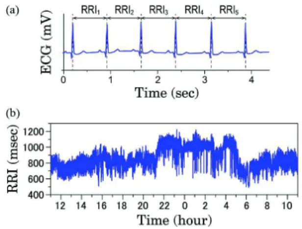
Fig. 2.Definition of R-R interval (RRI) and 24 hour heart rate

variability (HRV). In general HRV analysis, the R-peak in normal sinus rhythm is assumed. (a) The R wave can be detected as a sharp positive peak in the standard electrocardiogram (ECG), and the RRI is defined as the duration between successive R-waves. (b) 24 hour HRV (normal-to-normal R-R intervals) in a 31-yr-old male subject.

statistical physics and nonlinear dynamics have been ap-plied to HRV analysis [51]. The nonlinear indices which have been proposed include scaling exponents character-izing fractal and long-range correlation characteristics [16], [52], multifractal properties [22], Poincare´ plot-based indices [53], entropy measures [54]–[57], symbolic pattern statistics [55], [58] and non-Gaussian properties [23]. Some of these nonlinear indices are expected to provide complementary information on HRV characteris-tics contributing to better diagnosis and prognosis than conventional time and frequency domain indices.

With regards to a dynamical disease perspective [Fig. 1], the following aspects of the HRV dynamics should be considered as important: (1) common dynami-cal properties of HRV have been observed in healthy sub-jects even in daily life, when the measurements are performed, [23], [26], although these properties can de-pend on age [59], [60]; (2) these properties arise from endogenous HRV dynamics, not from behavioral and en-vironmental factors [23], [26]; and (3) an alteration of such properties are associated with morbidity and mortal-ity in cardiac patients [25], [28], [61], [62]. These proper-ties have been observed in long-range correlation [26], multifractality [22] and scale invariant non-Gaussianity [23]. These characteristics are evaluated based on multi-scale (or multiresolution) analysis, and have been exam-ined as mortality risk markers for cardiac patients. Moreover, some markers are suggested to be associated with overall sympathetic hyperactivity during daily life. Thus, multiscale analysis approaches could provide new insight into HRV dynamics.

In this section, we discuss multiscale characteristics of HRV and the key issues for evaluation of ANS func-tions, especially sympathetic activity thought to play an important role in the transition of the allostatic state. B. Frequency Domain HRV Markers and the Limitations

Frequency domain analysis based on Fourier power spectral density estimation is a widely used tool for the investigation of HRV [13]. HRV power spectral density serves to detect a number of physiological processes working at different and multiple time scales. In healthy subjects under controlled conditions, a typical power spectrum of HRV is comprised of two oscillating compo-nents in high-frequency (HF; 0.15 to 0.4 Hz) and low-frequency (LF; 0.04 to 0.15 Hz) bands [Fig. 3(b)], and a 1=f noise-like component in very-low-frequency (VLF;

below 0.04 Hz) band. The HF component reflects effects of respiration on heart rate, referred to as respiratory si-nus arrhythmia (RSA) while the LF component, associ-ated with so-called Mayer waves (approximately 0.1 Hz), represents oscillations related to regulation of blood pressure and vasomotor tone. The origin of the VLF com-ponent remains an open issue: it is however commonly thought to relate to hemodynamic functions [13], [43],

[63], [64], such as thermoregulation and kidney func-tion. For the noninvasive assessment of ANS functions, power of the HF component is taken as a marker for car-diac parasympathetic activity; the LF component is a marker for cardiac sympathetic activity, or both the sym-pathetic and parasymsym-pathetic influences, and the ratio of LF to HF power (LF/HF ratio) indicates sympathovagal balance, which is usually interpreted as reflecting the relative sympathetic predominance [13], [65]. In this view, an increase in LF power is assumed to indicate an increase in sympathetic activity, and a higher value of LF/HF ratio indicates a shift of sympathovagal balance toward sympathetic predominance.

It is generally accepted that HF power reflects RSA me-diated by the parasympathetic activity [66]. However, the origin and clinical significance of LF power have aroused considerable controversy. In short-term HRV recordings (! minutes) under experimental conditions affecting

Fig. 3.Frequency domain HRV analysis. (a) Time series of R-R

intervals in a 31-yr-old male subject (top) and its frequency band

components (3bottom rows). The time series was resampled at

evenly spacedintervals (2 Hz). The R-R time series was decomposed into high frequency (HF: 0.15 to 0.40 Hz), low frequency (LF: 0.04 to 0.15 Hz) and very low frequency (0 to 0.04 Hz) components. These components were obtained using the inverse Fourier transform of corresponding frequency

components. (b) Power spectral density of the R-R time series (a). (c) Assessment of the scaling exponent " of 24-h HRV. The power spectrum was estimated from the resampled time series at 2 Hz.

autonomic response, the relative power contribution of LF component is considered as a marker for sympathetic mod-ulation [65], [67]. However, many studies using pharmaco-logical, physiological and psychological manipulations affecting sympathetic activity on HRV have challenged the association of cardiac sympathetic activity with LF power [68], [69]. The available data have suggested that over a wide frequency range including HF and LF bands, the HRV power spectrum is mainly determined by the para-sympathetic system [70]. It has also been suggested that the LF power constitutes an index of baroreceptor reflex gain (or sensitivity) in mediating oscillations in blood pres-sure and vasomotor activity [71], [72].

More controversial was the interpretation of LF power and LF/HF ratio obtained from 24-hour ambula-tory HRV recordings in patients with a marked reduction in ventricular function. While in these patients, sympa-thetic activity was reported to be markedly elevated [48], a decrease in LF power and LF/HF ratio is more com-monly observed, and associated with increased risk of mortality [18], [73]. Therefore, clinical significance of as-sociation of cardiac sympathetic activity with LF power-related indices is questionable.

In addition to scale-specific behavior of HRV observed in HF and LF bands, it has also been proposed that HRV fluctuations show fractal, or scaling properties in the VLF band (G 0.04 Hz), related to long-range correlations [16], [17], [20], [59], [74], [75]. A time series is said to exhibit long-range correlations when the data points across widely separated times are correlated and the autocorre-lation function of the time series or its increments shows a power-law decay: Cð#Þ ! #$$_{, where # is the time lag} [76]. Although the general mathematical mechanism for generating long-range correlations is not clear, in some numerical studies of complex systems, long-range correla-tions emerge as a result of the collective behavior of mul-tiple interacting components, each with its own, specific and different characteristic time scales [77].

The conventional way to quantify long-range correla-tions is to use power spectral analysis. Although long-range correlated processes withSðfÞ ! f$" _{power spectra} have no characteristic time scale, such processes can be characterized by a scaling exponent " [Fig. 3(c)]. The 1=f" _{power spectrum over large time scales is related to} the power-law autocorrelation ð! #$$_{Þ by " ¼ 1 $ $} when 0 G $ G 1 [78]. By estimating the slope in a log-log plot of the 1=f"-type power spectrum, the scaling expo-nent " can be obtained. A representative stochastic pro-cess exhibiting monofractal behavior is fractional Brownian motion (fBm) as a generalization of Brownian motion [79]. This process is a Gaussian process BHðtÞ and self-similar in terms of statistical properties:

BHðatÞ ¼! jajHBHðtÞ, where “¼!” denotes equality of the probability distribution, 0 G H G 1 is a scaling exponent, called the Hurst exponent, and related to " by "_{¼ 2H þ 1. In addition, the increment process of fBm}

exhibits long-range correlation and is referred to as frac-tional Gaussian noise (fGn), with "¼ 2H $ 1.

In HRV analysis of healthy individuals, the value of " is close to one in young adults, and gradually increases with aging [59]. Moreover, an abnormal increase of " (9 1.5) has been reported to be associated with an in-creased risk of mortality in cardiac patients [61], [62]. To consider this phenomenon, it is important to note that the long-range correlated nature over the range of several tens of seconds to a few hours arises from endogenous HRV dynamics, not from exogenous effects such as be-havioral and environmental factors [26]. To explain the mechanism of the long-range correlated HRV, analogies with critical phenomena have been proposed [23], [24]. The characteristic features at the critical point of a phase transition are the divergence of relaxation time with strongly correlated fluctuations and the scale invariance in statistical properties. A healthy human heart rate has been confirmed robustly to show the 1=f"-type power spectrum. In addition, it is also reported that HRV in healthy individuals undergoes a phase-transition-like be-havior [24]. That is, highly correlated fluctuations are ob-served only during daily activity, and a breakdown of these characteristics occurs during prolonged, strenuous exercise and in the nocturnal sleep period.

In the scaling analysis of HRV, it is important to note that power spectrum analysis may provide spurious de-tection of scaling properties caused by nonstationarity of the time series [76]. The nonstationarity, such as a smooth baseline trend and heterogeneous statistical property, is known to introduce spurious scaling. To avoid such artifacts and to provide more accurate esti-mates of scaling exponents, alternative analysis methods have been developed, such as detrended fluctuation ysis (DFA) [16] and multiresolution time-frequency anal-ysis based on wavelet transform [80], [81]. In clinically oriented studies, the DFA has been frequently used, and some studies demonstrated its clinical significance (see [41] for a comprehensive review). On the other hand, multiresolution time-frequency analysis based on wavelet transform has also been recognized as a tool to study non-stationary signals [80], [81]. In this analysis, a time series is decomposed into different time-scale compo-nents. An advantage of wavelet analysis is that it can have a salutary effect called vanishing moments which eliminates smooth trends in the observed time series. Wavelet analysis can provide more detailed information about the time-varying properties of HRV. Therefore, it may be a useful tool to detect and predict fatal events. The ability of wavelet analysis to model and describe the scale-free properties of HRV temporal dynamics has been well documented in [23], [82]–[85].

C. Intermittent Fluctuations of HRV

In addition to 1=f" scaling as observed in fBm and fGn, multiscaling (multifractal) properties of HRV have

been studied mainly in the field of statistical physics [22], [82], [86]–[88]. Ivanov et al. reported, for the first

time, multifractality of HRV in normal subjects and re-duced multifractality in patients with congestive heart failure (CHF) [22]. Further, it has been suggested that multifractal HRV is associated with ANS functions and mainly with parasympathetic modulation [89], [90]. Re-cent methodological developments in multifractal analy-sis are expected to expand its potential applications to HRV analysis [83]–[85], [91], [92].

Multifractal analysis was initially introduced to study the so-called intermittency phenomenon of the fluid ve-locity field in fully developed turbulence [93]. The multi-fractality of the intermittent turbulent behavior is closely related to a multiplicative cascade process where the lo-cal energy on a given slo-cale is linked to lolo-cal energy on a larger scale via a random multiplier [94], [95]. The ob-served multifractality of HRV implies the intermittent nature of HRV fluctuations and is analogous to the multi-plicative cascade process [96].

A one-dimensional discrete time series based on the idea of the multiplicative cascade can be constructed as follows [97]: one starts with a discrete time series of Gaussian noise fXtg of length 2m _{where m is the total} number of cascade steps, and split the interval into two

equal subintervals. On each subinterval, the local stan-dard deviation (SD) is multiplied by random weightseY, where Y are independent Gaussian random variables

with variance %2=m and %* 0 is a shape parameter con-trolling the strength of non-Gaussianity. Each of the two subintervals is again cut in two equal subintervals and the process is repeated. After m cascade steps, the time

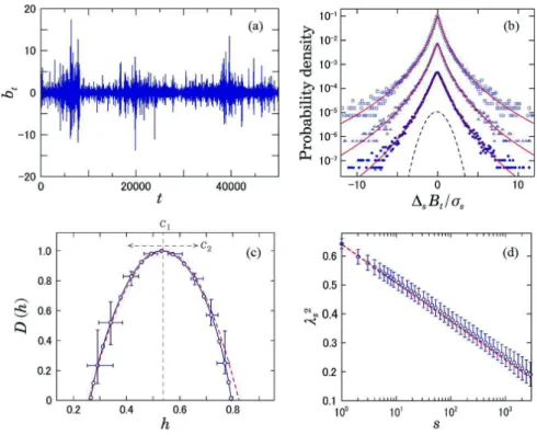
seriesfbtg is given by bt¼ Xtexp Xm j¼1 YðjÞ ðt$1Þ 2m$j j k (1)

where b,c is the floor function. As shown in Fig. 4(a), this process exhibits intermittent bursts due to the multi-plication of multiple random variables. One of the main tools to characterize these intermittent fluctuations has been multifractal analysis [e.g., Fig. 4(c)]. On the other hand, a remarkable property of the intermittent fluctua-tions is heterogeneity of variance, which results in non-Gaussian probability density functions (PDF’s) [Fig. 4(b)]. Thus, characterization of intermittent fluctuations is pos-sible through the analysis of the deformation process of

Fig. 4._{Characterization of intermittent fluctuations. (a) An example of an intermittent time series fb}tg generated by a multiplicative

cascade model (Eq. (1) with %2_{¼ 0:8}2_{, m ¼ 16). (b) Deformation of PDF’s of f!}

sBðtÞg, where BðtÞ ¼Ptk¼1bðkÞ and !sBðtÞ ¼ Bðt þ sÞ $ BðtÞ.

Standardized PDF’s for different scales are shown for (from top to bottom) s ¼ 1; 4; 16. In the solid lines, we superimposed the PDF’s approximated by a multiplicative log-normal model [Eq. (3) with a Gaussian kernel G]. For comparison, the dashed lines denote a Gaussian distribution. (c) The singularity spectrum DðhÞ of the integrated series fBðtÞg. DðhÞ was estimated from 64 samples using

p_{-exponent and p-leader based multifractal analysis with p ¼ 1 (see [8] for details). (d) Scale dependence of %}2

of f!sBðtÞg. Dashed lines

indicate theoretical predictions: %2

the non-Gaussian PDF’s across scales [Fig. 4(d)] [10], [97], [98]. Recently, the non-Gaussianity of HRV has been suggested as a marker potentially related to sympa-thetic cardiac overdrive [11], [25], [28]. Therefore, per-haps even more so than conventional HRV markers associated mainly with parasympathetic activity, this ap-proach may be useful to evaluate another important phys-iological function. In addition, long-range correlation, multifractality, and large non-Gaussian deviations are commonly observed near dynamical transition points [99], [100] [Fig. 1]. Therefore, such properties may be useful for finding early warning signals for fatal and cata-strophic events.

1) Multifractal Analysis—HRV as Multiplicative Cascades:

Multifractal analysis is able to characterize the fluctua-tions over time of the (ir-)regularity or singularity of a

signal XðtÞ, measured by a pointwise regularity (Ho¨lder) exponenth_{ðtÞ, by means of the so-called singularity}

spec-trum, defined as the fractal (Hausdorff) dimension of the set of time instances with the same regularity [101]:

DðhÞ ¼ dimH%tijhðtiÞ ¼ h

&: (2)

The practical counterpart enabling the estimation of

DðhÞ from data termed multifractal formalism relies on the characterization of scaling behavior of higher order statistics.

Many methods have been proposed to estimate the singularity spectrumDðhÞ from observed time series (cf. [84] for a review). As for the multifractality of HRV, wavelet transform modulus maxima (WTMM) methods [38] and multifractal detrended fluctuation analysis (MFDFA) [39], [40] have been mainly employed [22], [82], [86], [87], [89], [90].

Most recently, a framework has been proposed that extends the wavelet based analysis of self-similar pro-cesses and the estimation of the Hurst parameter H to

the analysis of multifractal scaling and to the estimation of the multifractal spectrum D_{ðhÞ [8]. It is referred to as} p-exponent and p-leader based multifractal analysis, and

it permits, beyond the limitation of the Ho¨lder exponent (*0), accounting for negative regularity, widely ob-served in the real-world time series and notably in HRV. Thus, this approach could provide a new and powerful tool to examine the multifractality of HRV, as shown in Fig. 6(d).

Matlab code implementing the wavelet analysis of self-similarity and multifractality is available at http:// www.irit.fr/~Herwig.Wendt/software.html#wlbmf.

2) Non-Gaussian Properties of HRV: In studies of

devel-oped turbulence and non-equilibrium systems exhibiting intermittent fluctuations, it has been demonstrated that

the observed non-Gaussian probability distributions with fat tails are often described effectively by a superposition of Gaussian distributions with fluctuating variances [102]. Based on this framework, the observed distribu-tion can be approximated by

PðxÞ ¼ Z1 0 1 (PL x ( ( ) Gðln (Þdðln (Þ (3)

wherePL is the standard Gaussian distribution and G is a distribution describing the fluctuation of the standard de-viations. In the analysis of intermittent fluctuations, we focus mainly on the estimation of the variance of G and

its scale dependence [102].

Based on this framework, Kiyono et al. proposed a

multiscale probability density function (PDF) analysis in-cluding a detrending procedure [23], [98]. The proce-dure of this analysis is as follows: (1) Time series of R-R intervals are interpolated and resampled at 4 Hz, yielding interpolated time seriesfbtg. After subtracting the mean from the interpolated time series, integrated time series fBðtÞg are obtained by integrating fbðtÞg over the entire series length. (2) The integrated time series fBðtÞg are divided into overlapping segments of length 2s with

50% overlap, where s is the scale of coarse graining

(s¼ 25 sec in Fig. 5). In each segment, the local trend is eliminated by third-order polynomial fit. (3) Coarse grained variation !sBðtÞ is measured as the increment with a time lag s of integrated and detrended time

se-ries. (4) f!sBðtÞg is standardized by its standard devia-tion to quantify the PDF. Then, the non-Gaussianity index %s is estimated based on the qth-order moment of f!sBðtÞg as %2 sðqÞ ¼ 2 qðq $ 2Þ ln ffiffiffi ) p E +!sBðtÞ + ++q , -2q2" qþ1 2 . / 0 B @ 1 C A 2 6 6 4 3 7 7 5 (4)

where E_{ðXÞ is the expectation value of X and " is the}

Gamma function [97]. In previous studies [25], [28], %s is estimated based on the 0.25th-order moment ðq ¼ 0:25Þ to emphasize the center part of PDF. In this anal-ysis, the observed non-Gaussian shape [Fig. 4(b)] at each scale is quantified by the non-Gaussianity index %s defined as the standard deviation of ln ( in (3), where

G is assumed to be a Gaussian. The greater the %s, the greater the proportion of large deviation than what is expected from the Gaussian distribution.

Using this method, Kiyono et al. reported robust

scale-invariant properties in non-Gaussian distributions observed in healthy human HRV spanning the range of

about 20–2000 beats, which were preserved not only in a quiescent condition, but also in a dynamic state where the mean level of the heart rate was dramatically chang-ing [23]. In addition, in patients with CHF, increased non-Gaussianity at scale of 40 beats of 24-hour ambula-tory HRV predicts increased mortality risk, while none of the conventional HRV indices, including those reflect-ing vagal heart rate control, were predictive of death

[25]. Moreover, Hayano et al. reported that, in patients

after AMI, an increased non-Gaussianity index %25 sec at a scale of 25 sec is associated with increased cardiac mortality risk, and its predictive power is independent of clinical risk factors and of other HRV predictors [28].

The aspects characterized by %25 secare related to am-plitude modulation properties of LF component as shown in Fig. 3(a). The detrending procedure in multiscale PDF

Fig. 5.Representative examples of non-Gaussian heart rate fluctuations during the daytime in a healthy subject and a congestive

heart failure patient. Time series of normal-to-normal R-R intervals (top row), standardized time series of coarse grained heart rate variations f!25 secBðtÞg (middle row), and standardized PDFs of !25 secBðtÞ (bottom row). Estimated values of the non-Gaussianity index

%25 secare shown in each panel in the bottom row. The solid lines represent the PDF approximated by a multiplicative log-normal

model [(3) with a Gaussian kernel G].

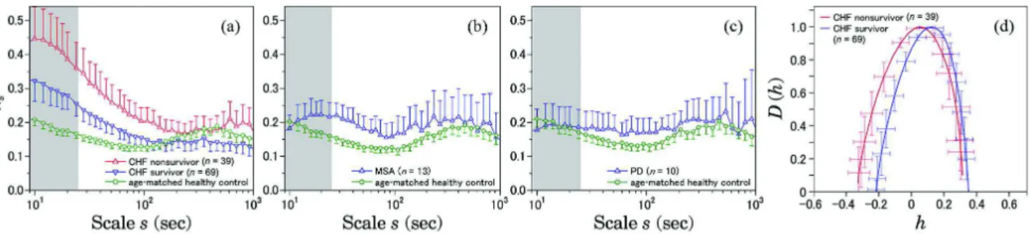
Fig. 6.Scale dependence of the non-Gaussianity index %2

sand Multifractal spectrum DðhÞ of daytime HRV (12:00-1800). The result for:

(a) congest_{ive heart failure (CHF) patients, both for survivors ðn ¼ 69Þ and non-survivors ðn ¼ 39Þ within the follow-up period of} 33 0 7 months; (b) multiple system atrophy (MSA); and (c) Parkinson disease (PD) patients. Age-matched controls were selected from a database of healthy subjects. Error bars indicate 95%-confidence intervals of the group means. The gray shaded range corresponds to low-frequency band ðsG25 secÞ. Marked increases in %2

sin the gray shaded scales are observed only in CHF patients, particularly

non-survivors (a). DðhÞ are estimated in the range of 10–200 sec using p-exponent and p-leader based multifractal analysis with p ¼ 1 (see [8] for details). These figures are modified versions from [11].

analysis acts as a high-pass filter that removes low fre-quency components below a given time scale, and the calculation of partial sums (or increments of integrated series) acts as a low-pass filter. In the estimation of %25 sec, the combination of these procedures acts as a band-pass filter that allows mainly the LF component to pass. The increased %25 secindicates an increase in ampli-tude heterogeneity of LF oscillation as seen in Fig. 5 (middle rows). Note that the %25 seccan change indepen-dently of the value of LF power. Thus, the %25 sec can provide complementary information beyond conventional frequency domain indices.

As for the association of %25 sec with the ANS func-tions, the following facts should be considered: (1) The HRV in the scales corresponding to HF and LF bands are mediated almost exclusively by neural autonomic mecha-nisms [13], [103]. (2) The %25 sec showed no substantial correlation with the HRV indices reflecting vagal heart rate regulation [25], [28]. (3) %25 secwas decreased in post-AMI patients taking beta-blockers suppressing the sympa-thetic influence [28]. Based on these facts, Hayano et al.

suggested that %25 sec captures heart rate fluctuation at least partly mediated by intermittent activations of cardiac sympathetic activity [28].

In addition, in the study of daytime HRV in patients with multiple system atrophy (MSA) and with Parkinson disease (PD), it is reported that a marked increase in non-Gaussianity on a relatively short time scale observed in CHF patients was not observed in these patients with sympathetic dysfunction [11]. Both MSA and PD are pro-gressive neurodegenerative disorders, although auto-nomic lesions in MSA are caused by preganglionic sympathetic failure [104], and those of PD are ganglionic and postganglionic [105], [106]. As shown in Fig. 6, com-pared with an age-matched healthy control group, mean values of %s in CHF patients, especially nonsurvivors in comparison to survivors during the follow-up period, dis

-play marked increases in relatively small scales covering

the LF band. On the other hand, as shown in Fig. 6(b)

and (c), such marked increases were not observed in MSA and PD patients. This result also supports the view that an increase of %25 sec could be a hallmark of overall cardiac sympathetic overdrive detectable with ambulatory HRV monitoring.

The fact that heart rate dynamics of CHF patients with elevated sympathetic activity exhibit a marked in-crease in non-Gaussianity and its decays with scales within LF and VLF ranges suggests a sympathetic origin for HRV intermittency. In these scales (G 200 sec), heart rate dynamics reflect cardiovascular regulation by neural, humoral, and thermal influences [107]. These subsystems are considered to be compensatory; therefore, it is likely that only simultaneous failure of all these subsystems op-erating on multiple time scales, compatible with the re-ciprocal of cascade steps “j” in (1) could result in

sympathetic overdrive, leading to intermittent heart rate

fluctuations with large deviations. We propose that such a multiplicative picture would provide a deeper physio-logical understanding of the nature of sympathetic func-tion [11]. As shown in Fig. 6(d), intermittent nature of HRV in CHF patients may also be characterized by mul-tifractal analysis. Also, the fact that HRV of non-surviving CHF patients exhibit stronger LF intermittency than that of surviving patients [Fig. 6(a)] would indicate a relation-ship between appearance of the HRV intermittency (due to sympathetic overdrive as a control parameter) and a pathological transition [Fig. 1]. The same scenario also applies to AMI patients in [28].

D. Remarks and Other Methods

Sympathetic nervous system activity is thought to be an important factor in many health problems, not only in cardiovascular diseases but also in the development of a wide variety of chronic illnesses [108]. Therefore, mul-tiscale analysis characterizing the intermittent nature of HRV may have widespread applications in various fields of health management. Among HRV indices that have been suggested as markers of sympathetic activity, an in-creased non-Gaussianity of HRV may reflect hazardous effects of elevated cardiac sympathetic activity in cardiac patients. In addition, some other nonlinear markers not mentioned in this paper, such as approximate and sample entropies, have been suggested to be associated with sympathetic activation [109], [110]. Moreover, multiscale entropy analysis [36], [37] and other multiscale tools, such as empirical mode decomposition [111] may have potential clinical applications. However, to establish as-sociations between sympathetic activity and the clinical significance of these approaches, systematic validation and further studies on a large scale data are yet required.

I I I . S P ON T A N EO U S P H YS I C A L A C T I V I T Y

A. Alterations of SPA in Psychiatric Diseases

In the fields of psychiatry and mental healthcare, pre-vention and early interpre-vention are crucially important and widely accepted as effective strategies to reduce the number of patients with serious psychiatric disorders and ultimately medical/healthcare related costs [112]–[114]. In order to develop a reliable and effective strategy based on clinical evidence, the identification of an objective biomarker for psychiatric disorders is essential because it could contribute to the early detection of warning signs for pathogenic and/or pathological changes resulting in the development of these illnesses [115]. However, such an objective measure has not been fully developed.

The recent development of information and commu-nication technologies, such as wearable/mobile devices, provides massive longitudinal, non-medical data from our daily lives (e.g., physical activity, heart rate, GPS,

etc.), which are thought to include useful information on our physiological and/or pathological conditions. While the extraction of pathological information available for clinical use is still challenging, many researchers have re-cently studied and reported promising outcomes [116]– [118]. In this section, we introduce examples of objective evaluation of psychiatric disorders based on physical ac-tivity easily assessed by using a wearable device.

1) Behavioral Abnormalities in Psychiatric Disorders:

Physical activity can be continuously monitored in a quantitative and noninvasive way, e.g., through the use of a wrist watch- type or band-type acceleration sensor, a method referred to as actigraphy. This type of device has

the capability of detecting small changes in bodily/wrist acceleration so that even slight movements by the sub-jects are registered. Therefore, the data recorded include information on both conscious and unconscious behav-iors in daily life. In this review, we call this type of lon-gitudinal behavioral data spontaneous physical activity (SPA).

Behavioral alteration is one of the cardinal signs of psychiatric disorders, and many psychiatric disorders, in-cluding depression, indeed have diagnostic criteria which require an assessment of altered physical activity [15]. For instance, one of the known disease signs of depres-sion is psychomotor retardation, involving a recognizable alteration in physical activity such as slowing down of movement [119]. Therefore, behavioral dynamics is con-sidered to contain rich information on pathological symptoms of psychiatric disorders and is thought to be useful for objective diagnosis of disorders.

In order to characterize behavioral abnormalities, in-cluding chronobiological disturbances, basic statistics (e.g., mean and variance) and periodicities (by, e.g., cosinor method or Fourier analysis) of SPA have been tradition-ally evaluated. For example, reduced daily activity levels have been reported in patients with major depressive dis-order (MDD) [14], [15] and schizophrenia [120], [121]. On the other hand, increased activity levels were shown in patients with attention-deficit hyperactivity disorder [122], [123] and patients with bipolar disorder (BD) dur-ing manic phases [124]. In addition, significant associa-tions of these statistics with clinical variables have also been confirmed [125]–[127]. From the viewpoint of dy-namical properties of SPA, Haugeet al. examined an

en-tropy measure to show the increase in complexity of SPA in schizophrenia [120]. Indic et al. examined the scaling

behavior of amplitudes of SPA on multiple time scales and reported altered scaling behavior in BD as well as as-sociations with clinical states, indicating the utility of monitoring SPA for objective evaluation of pathological states of BD [128].

The direct connection between alterations in these traditional measures and the underlying pathophysiology is unknown, but several studies using neuroimaging

approaches have recently suggested the existence of asso-ciations of SPA with brain structures or functions in the motor control systems [129]–[132]. For example, altered associations of SPA with structures and functions of mo-tor regions of brain, including anterior cingulate cortex, supplementary motor area, and thalamus, have been re-ported in schizophrenia patients [129], [131], [133]. In addition, a relationship between dysfunction of cortico-basal ganglia pathways in white matter and the patho-physiology of hypokinesia in schizophrenia has been reported, suggesting that structural disconnectivity could lead to disturbed motor behavior in schizophrenia [132]. Studies about MDD have also demonstrated the link be-tween psychomotor retardation and white matter integ-rity of the motor system [134], [135]. These reports manifest the existence of underlying neurological bases for SPA.

B. On-off Intermittency and Scale-Invariance in SPA As detailed in this subsection, Nakamura et al.

re-cently studied the dynamical properties of SPA and dis-covered robust statistical laws of behavioral organization, specifically how resting and active periods derived from physical activity data are interwoven into daily life [1], [2], [31]. Furthermore, they reported alterations in the resting period statistical law in patients with MDD [1] and schizophrenia [31] reflecting increased intermittent bursts in activity counts characterized by reduced activity levels associated with occasional bursts of physical activ-ity. These studies manifest that the quantitative and ob-jective evaluation of intermittency of physical activity could provide appropriate behavioral measures capable of probing alterations in pathological states in psychiatric disorders.

1) Intermittent Nature of SPA and its Alterations: Fig. 7

shows typical fluctuations of SPA in a healthy subject and in a patient with MDD. In the healthy subject [Fig. 7(a)], a clear circadian rest-activity cycle is observed, while in the MDD patient [Fig. 7(b)], this rhythmic pat-tern is notably disrupted, reflecting the reported chrono-biological abnormality in depression [14]. During the daytime, physical activity of the healthy subject is charac-terized by consistently higher activity levels, whereas the MDD patient exhibits intermittent bursts in activity counts with more episodes of slowing down or cessation of movements [1], [31]. As mentioned below, the inter-mittent burst is a significant dynamical feature of physical activity and its alteration is a robust and effective indica-tor for behavioral abnormalities observed in psychiatric disorders.

2) Statistical Laws of Behavioral Organization: In order to

characterize the intermittent patterns in physical activity, Nakamuraet al. evaluated the cumulative probability

dis-tribution PCðx * aÞ of durations a of both resting pe-riods, where the activity counts were successively lower

than a certain predefined threshold value (e.g., an over-all average of non-zero activity counts), and of active periods, where the counts were successively higher than the threshold values [1], [2] [the bottom panels in Fig. 7(a) and (b)]. The robust statistical laws they found in healthy subjects [1], [2], against factors such as differ-ence in study populations and choice of different thresh-olds, were the power-law distribution PCðx * aÞ ! a$$ with the scaling exponent $! 1:0 for the distributions of resting period durations [Fig. 7(c)] and the stretched ex-ponential functional form PCðx * aÞ ¼ expð$*a"_{Þ with} the stretching parameter "! 0:5 for the distribution of active period durations [Fig. 7(d)]. In addition, they re-ported that these statistical laws found in healthy humans were shared by wild-type mice (i.e., no significant differ-ence in values of the scaling exponent $ and the stretch-ing parameter "), suggestive of the presence of an underlying principle governing behavioral organization, or

behavioral switching, across species [2]. Furthermore, a significant decrease in $ of resting period distributions among humans with MDD or schizophrenia [1], [31] and mice with deficiency in a circadian clock gene (Period 2) [2] has also been reported. These findings indicate that al-terations in intermittency of behavioral dynamics charac-terized by $ are useful for describing abnormalities in SPA observed in psychiatric disorders. Another important point to be emphasized is the possibility that the cross-species translation provided by the statisitcal law of behavioral organization may play a crucial role in bridging the gap between specific genetic substrates and behavioral endo-phenotypes in psychiatric disorders [136], [137].

3) A Model for on-off Intermittency in Behavioral Organiza-tion: In order to elucidate the underlying mechanisms of

the alteration in resting period distributions, a mathe-matical model based on queuing theory [12], [124], which models a decision-making strategy for selection of

Fig. 7.Fluctuations in spontaneous physical activity and their statistical laws of behavioral organization (modified from [1], [2]).

Illustrative examples of physical activity data for a healthy adult (a), and a patient with major depressive disorder (MDD) (b) over

three consecutive days (top panels). These data were measured by a watch-type device (Ambulatory Monitors Inc., Ardsley, NY, USA) worn on the wrist of their non-dominant hand. The zero-crossing mode, which measures counts of events in which an acceleration signal crosses a zero level within a predefined time (e.g., 1 min), is used. The middle panels are magnifications of the top panels with 4 h periods during the third day. The overall average of non-zero activity counts was used as the threshold (horizontal dotted line), and the period during which the activity counts were successively below or above the threshold is defined as a resting or active period, respectively (bottom panels). (c) Cumulative distributions PCðx * aÞ of resting period durations a for healthy adults (open

circles) and MDD patients (blue filled squares). Straight lines are eye guides with the overall mean values; the power law distribution with $ ! 1:0 for healthy adults and $ ! 0:7 for MDD patients, respectively. The green curve indicates a random case (i.e., an exponential functional form). (d) The same as (c) but for active period durations. The stretched exponential functions were nicely fitted to the active distributions. Error bars indicate standard error of the mean.

a biological “cue” to response [4], was considered. This model is based on the following assumptions; spontane-ous movements in animals would be triggered by contin-uously presented internal or external demands and/or stimuli (e.g., appetite, emotion, etc.); on the basis of their biological importance, one demand/stimuli is prob-abilistically chosen either consciously or unconsciously. This decision-making process can be modeled well by a stochastic priority queuing model. In [4], we demon-strated that a strategy where each demand/stimuli is probabilistically chosen every time in proportion to its biological importance can explain the unique statistical law of resting periods with $ ! 1:0. Mathematically, with the probability of response to a demand/stimuli with priority x given by _{QðxÞ ! x [black line in Fig. 8(a)],}

the cumulative distribution of durations of resting pe-riods is analytically derived to follow the power-law func-tional form [12] with the exponent $¼ 1 [Fig. 8(b)]. In contrast, the decrease of $ observed in MDD, schizo-phrenia, and BD during the depression phase [Fig. 8(c); see III-C below] can be reproduced by assumingQðxÞ !

x% with % greater than unity (e.g., %¼ 1:4) [blue curve in Fig. 8(a)]. This assumption implies that a demand/ stimuli with higher priority is preferentially selected, giv-ing rise to a fatter distribution tail and frequent episodes

of longer resting periods, generating a more intermittent sequence of onset of activity bursts [Fig. 8(c)]. Also, the increase of $, observed in a patient with BD during a manic episode, can be modeled by assuming % smaller than unity (e.g., %¼ 0:8) [red curve in Fig. 8(a) and (d)]. Based on the findings for mice with deficiency in Period 2 also showing decreased $ [138], [139], we dis-cussed [4] that these strategic changes in decision-making —preferential selectivity to demands and/or stimuli with higher priority—may be related to reinforcement of re-warding neural networks induced by dysfunction of the dopamine and/or glutamatergic systems.

C. Towards Monitoring and Early Detection of Psychiatric Disorders

1) ILD of SPA in Bipolar Disorder: Bipolar disorder is a

major psychiatric disorder demonstrating recurrent and alternating periods of manic (or hypomanic), depressive, and mixed episodes, with varying intervals [119], [140], [141]. Mania, a period of elevated or irritable mood, as well as increased energy (overactivity) and a decreased need for sleep, is the defining feature of BD. On the other hand, like MDD, depressive episodes are character-ized by lack of interest, loss of energy, insomnia, fatiga-bility, and suicidal thoughts. The most prominent feature

Fig. 8.Sequences of resting period durations and their model (modified from [4]). (a) Probability density function_{QðxÞ ! x}%_for

choosing a demand/stimulus with physiological priority x. The sequence of onset of activity bursts (resting durations) derived from

physic_{al activity of a (b) healthy adult ð$ ! 1:0Þ, (c) a bipoloar disorder (BD) patient in the depressive phase ð$ ! 0:7Þ, and (d) in the}

hypomanic phase. The sequence of waiting times simulated from the priority stochastic queuing model with (b) % ¼ 1:0 (i.e., $ ¼ 1:0), (c) % ¼ 1:4 (i.e., $ ! 0:7), and (d) % ¼ 0:8 (i.e., $ ! 1:25) are also shown. The simulated sequences of waiting time were generated on the base of the stochastic priority queuing model [12] with a priority list comprising L ¼ 10 demands, where a priority parameter xiði ¼ 1; . . . ; LÞ

chosen from a uniform distribution +ðxÞ ¼ Uð0; 1Þ is assigned to each demand. At each time step, one demand is selected from the list (in the brain) according to_{QðxÞ ! x}%_{for execution (or act), and then removed from the list. At that moment, a new demand is added to}

the list with a priority randomly selected from +ðxÞ. The probability that a demand with priority x is executed at time t is given by fðx; tÞ ¼ ð1 $QðxÞÞt$1QðxÞ, and the average waiting time of a demand with priority x is obtained by averaging over t weighted with fðx; tÞ, giving rise to #ðxÞ ¼P1

t¼1tfðt; xÞ ¼ 1=$ðxÞ 1 1=x%. Analytically, with the conservation law of probability ð+ðxÞdx ¼ Pð#Þd#Þ, the waiting time

distribution of the demands is given by Pð#Þ 1 +ð#$1=%_Þ=#1þ1=%_{. Note that each vertical line separates the successive waiting time of demands}

of BD is the switching dynamics between depressive and manic phases. Elucidating the underlying mechanism of these sudden changes in pathological states is important as it would contribute to the precise and reliable predic-tion of the timing of these transipredic-tions. This in turn would lead to the development of timely and efficient clinical interventions, and novel treatments aimed at the prevention of suicide and decreasing the risk of issues with social relationships, loss of job and financial prob-lems. However, little attention has been given to these sorts of dynamical features (clinical phase transitions) of

pathological states in BD.

A longitudinal study design allows us to investigate dynamical aspects in pathological states during the period of clinical phase transitions in BD, along with inter-relationships between psychological and behavioral vari-ables. Indeed, studies examining BD using longitudinal designs have demonstrated dynamical changes related with phase transitions in subjective mood [142], [143], physical activity (including sleep and circadian rhythm) [144], [145], and biochemical variables [146].

Nakamura et al. recently measured ILD of SPA and

self-reported symptoms in bipolar patients (type-II) to cap-ture clinical phases transitions [3]. Fig. 9(a) and (b) repre-sent an example of physical activity data and subjective mood scores continuously monitored over almost one year, respectively, including a period of well-identified clinical phase transition. The activity levels during around 110– 140 days were consistently low with worsening of mood, indicative of a depressive episode. After this period, the mood scores gradually increased and then reached at the maximum score (the patient rated the best) on day 165. In parallel with this rapid mood change, the activity levels in-creased, manifesting the transition from the depressive phase to manic phase. The physical activity [labeled “A” in Fig. 9(a)] during the depressive phase showed frequent in-termittent bursts in the activity counts during the daytime [Fig. 9(d)], while the data [labeled “B” in Fig. 9(a)] in the manic phase was characterized by more sustained higher activity levels [Fig. 9(e)] [3].

In this subsection, we demonstrate the possibility to objectively monitor changes in pathological states based on alterations of behavioral dynamics (i.e., intermit-tency) and further discuss the detection of early signs for clinical phase transition.

2) Objective and Continuous Monitoring of Pathological States: Application of the method for behavioral

organiza-tion (see Fig. 7) during the clinical phase transiorganiza-tion re-vealed that the resting period distributions in both depressive and hypomanic phases took a power-law form

PCðx * aÞ ! a$$ _{over almost two decades (from 2 min to} 100 min), with considerable difference in their scaling exponent [$¼ 0:85 for the data during depressive phase shown in Fig. 9(d) and $¼ 1:22 for the data during hypo-manic phase shown in Fig. 9(e)]. The increase in longer resting periods in the depressive phase, like MDD,

suggests more episodes of slowing down or cessation of movement in depressive phase than in hypomanic phase.

The continuous nature of physical activity data allows us to evaluate daily changes in values of $ in a continu-ous fashion [Fig. 9(c)]. The objective behavioral index $ can distinguish the differences in pathological states in BD; the values of $ were lower in depressive phase than those in hypomanic phase. In addition, the low-frequency fluctuations (9 7 days) in the value of $ demonstrated the significant concurrent association with self-reported mood scores and the values of $ [3]. This indicates the possibility of quantitatively and continuously capturing manic-depressive phase transitions from physical activity monitored using a wearable device.

3) Detection of Early Signs for Pathological Transitions From the Viewpoint of Dynamical Systems: Investigation

into a theory for aperiodic alterations between depressive and manic episodes, by developing a dynamical model, may help elucidate the underlying mathematical mecha-nisms of the pathological phase transitions in BD and de-velop novel prediction methods, leading to timely and effective interventions.

The most prominent dynamical feature of BD is the coexistence of two extreme mood states (depression and mania) and oscillating/switching dynamics between them with unequal durations of each episode [143]. In addi-tion, clinical observations suggest that this aperiodicity in transition periods is determined by the interaction be-tween the biological mechanisms generating periodicity and environmental and psychological stresses in daily life [144], [147]. These complex and nonlinear dynamical phenomena are reminiscent ofbistability. Although other

dynamical models could be considered to describe the al-ternating phenomena between manic and depressive states [143], we start from hypothesizing a bistable sys-tem as a simple model to explain the switching mecha-nism. Indeed, by proposing a mathematical model with bistability, Goldberter successfully simulated the recur-rent and alternating switching dynamics between depres-sion and mania, together with the antidepressant effects clinically observed [148] (e.g., a transition to mania or rapid cycling triggered by antidepressants [149]).

Bifurcation of the bistable system reproduced the phenomena clinically observed in patient with BD well. If the same mechanism exists in actual pathological tran-sitions, there is a possibility to detect a tipping point of pathological transitions by evaluating the dynamical fea-tures of fluctuations in physiological parameters (e.g., mood and/or physical activity) because the system dis-plays complex and unique fluctuations around a bifurca-tion point [32]. Fig. 10(a)–(c) shows potential landscapes illustrating a bifurcation phenomenon of a bistable sys-tem as a model for pathological cycling in BD. Under the condition where a control parameter governing the dy-namics of the system is sufficiently close to a bifurcation point, the steady states (potential wells) become unstable,

and the system can no longer remain at these states, start-ing to fluctuate in a unique manner [Fig. 10(b)]. There-fore, the evaluation of dynamical features of fluctuations in state variables allows us to detect a tipping point of pathological transitions, like the dynamical disease sce-nario in Fig. 1. For example, critical slowing down is

known as a characteristic dynamical phenomenon emerg-ing in the vicinity of a phase transition or a critical point [32], indicating the occurrence of bifurcation in the un-derlying systems. These early warning signs are com-monly observed in a variety of fields from economics to climate systems [32], [150]–[153]. Systems showing

Fig. 9.Dynamics of spontaneous physical activity and subjective mood during clinical phase transitions in bipolar disorder (BD)

(modified from [3]). (a) A double-plot actogram of physical activity data of a patient with BD over 333 days. For presentation

purposes, the activity data were converted into resting and active periods and then color coded according to the corresponding value of $ [see (c)]. (b) Fluctuations in subjective mood scores reported by the patient every night, ranging from the 0 (the worst) to 10 (the best). The clinical phase transition from a depressive phase to a hypomanic phase occurred during the period between days 140–150. (c) The continuous evaluation of the scaling exponent $ of resting period distributions. Here, the value of $ was continuously estimated by using a sliding window of 7-day width by shifting 1 day [red filled circles in (c)]. The trend of $ [blue curve in (c)] significantly traced pathological changes of depressive-manic cycles rated by subjective mood [3]. The physical activity data during depressive phase (d) and manic phase (e), labeled “A” and “B” in the panel (a), respectively, are shown in (d) and (e). Their magnification with 4 h periods during the third day is also shown. The value of $ was 0.85 and 1.22, respectively.

critical slowing down are theoretically characterized by a decreasing rate of recovery from small perturbations (slowness), which results in the accumulation and persis-tence of perturbations over time, leading to increases in local variance and autocorrelation around critical points [32]. Fig. 10(e) as applied to the BD transition shows the changes in autocorrelation coefficients obtained by fitting an autoregressive model of order 1 [i.e., AR(1) model] to the data of $ [shown in Fig. 10(d)] within a sliding win-dow of size 10 days. During the transition period from de-pressive to manic phase (from 130–150 days), the autocorrelation coefficients of daily fluctuations of $ gradually increase, possibly giving rise to an early warn-ing sign for the phase transition. On the other hand, dur-ing clinically “stable” states in depressive and manic phases, the decrease of correlation coefficients to around zero value can be observed. This implies that the state of the system randomly fluctuates around a stable well [Fig. 10(a) or (c)]. This example suggests the possibility of detecting early warning signs for pathological transi-tions by evaluating the dynamical features of SPA, and also the viability of utilizing biomedical ILD to empiri-cally study disease dynamics, i.e., dynamical disease.

I V. S U M M A R Y A N D F U T U R E

D I RE C T I O N S

In this paper, we have shown the application of multi-scale analysis to two types of intensive longitudinal bio-medical signals, i.e., HRV and SPA time series. Recent advances in wearable and/or biomedical sensing technol-ogies [5]–[7] are enabling us to collect these data with large temporal scales up to days and months during daily life. Thus, it is now timely to start thinking about the rig-orous “use” of this type of data. In particular, it is consid-ered important to begin investigation into how to robustly characterize their statistical and dynamical prop-erties and how to practically utilize the analytical results in medicine and healthcare.

It was shown that these ILD indeed have robust char-acteristics unique to various multiscale complex systems, and that some parameters for multiscale complexity are in fact altered in pathological states, indicating potential usability as new types of ambient diagnostic and/or prog-nostic tools. For example, parameters characterizing in-creased intermittency (like %s; Section II) of HRV are found to be potentially useful in detecting abnormalities in the state of the autonomic nervous system, in

Fig. 10.A bifurcation phenomenon of a bistable system and early warning signs for clinical phase transitions in bipolar disorder (BD).

(a) and (c): the potential landscapes for a depressive phase (a) and a manic phase (c). (b) is an illustration of a potential function at

the bifurcation point (e.g. saddle node bifurcation). When the control parameter of the system is sufficiently close to the bifurcation

point, the steady statesbecome unstable and the most unstable direction in phase space dominates the behavior of the system. This direction is determined by the eigenvector of the Jacovian corresponding to the eigenvalue for which the eigenvalue becomes zero real valued. Around this point, fluctuations with unique dynamical properties (e.g., critical slowing down) can be observed. (d) The fluctuations in $ around the period of the phase transition from depression to mania. (e) The alteration in autocorrelation coefficients obtained by fitting an autoregressive model of order 1 [AR(1) model] to the data of $ within a sliding window of size 10-days. The locations where the values of autocorrelation coefficient approach to zero may correspond to the “stable” depressive and manic phase [labeled “(a)” and “(b)”] as illustrated in panel (a) and (b), respectively.