HAL Id: hal-00437293
https://hal.archives-ouvertes.fr/hal-00437293
Submitted on 30 Nov 2009
HAL is a multi-disciplinary open access
archive for the deposit and dissemination of
sci-entific research documents, whether they are
pub-lished or not. The documents may come from
teaching and research institutions in France or
abroad, or from public or private research centers.
L’archive ouverte pluridisciplinaire HAL, est
destinée au dépôt et à la diffusion de documents
scientifiques de niveau recherche, publiés ou non,
émanant des établissements d’enseignement et de
recherche français ou étrangers, des laboratoires
publics ou privés.
Fast and robust dominant point detection on digital
curves
Thanh Phuong Nguyen, Isabelle Debled-Rennesson
To cite this version:
Thanh Phuong Nguyen, Isabelle Debled-Rennesson. Fast and robust dominant point detection on
digital curves. International Conference on Image Processing, Nov 2009, Caire, Egypt. pp.953-956.
�hal-00437293�
FAST AND ROBUST DOMINANT POINTS DETECTION ON DIGITAL CURVES
Thanh Phuong Nguyen, Isabelle Debled-Rennesson
LORIA Nancy, Campus Scientifique - BP 239
54506 Vandoeuvre-l
e
`
s-Nancy Cedex, France
ABSTRACT
A new and fast method for dominant point detection and polygonal representation of a discrete curve is proposed. Starting from results of discrete geometry [1, 2], the notion of maximal blurred segment of widthν has been proposed, well adapted to possibly noisy and/or
not connected curves [3]. For a given width, the dominant points of a curveC are deduced from the sequence of maximal blurred
seg-ments ofC in O(n log2n) time. Comparisons with other methods
of the literature prove the efficacity of our approach.
Index Terms— corner detection, dominant point, critical point
1. INTRODUCTION
The work on the detection of dominant points started from the re-search of Attneave [4] who said that the local maximum curvature points on a curve have a rich information content and are sufficient to characterize this curve. Therefore, these points play a critical role in curve approximation, image matching and in other domains of machine vision. Many works have been realised about the dominant point detection and an interesting survey is presented in [5]. Several problems have been identified in the different approaches: time com-putation, number of parameters, selection of start point, bad results with noisy curves, ...
In this paper, we present a new fast and sequential method issued from theoretical results of discrete geometry, it only requires to fixe one parameter, it is invariant to the choice of the start point and it works naturally with general curves : possibly being noisy or dis-connected. It relies on the geometrical structure of the studied curve obtained by considering the decomposition of the curve into maxi-mal blurred segments for a given width [3].
In section 2, we recall theoretical results of discrete geometry used in this paper to analyse a curve. The section 3 describes our method for dominant point detection. Finally, the section 4 presents experimental results and comparisons with other methods.
2. DECOMPOSITION OF A CURVE INTO MAXIMAL BLURRED SEGMENTS
The notion of blurred segment [2] relies on the notion of arithmetic discrete line [6]. An arithmetic discrete line, notedD(a, b, µ, ω),
is a set of points (x, y) that verifies this double inequation: µ ≤ ax − by < µ + ω with a, b, µ, ω integer parameters. A width ν
blurred segment is a set of integer points which belong to a discrete lineD(a, b, µ, ω) verifying ω−1
max(|a|,|b|) ≤ ν. The notion of width This work is supported by the ANR in the framework of the GEODIB project, BLAN06-2 134999.
ν maximal blurred segment, used in this paper, was proposed in [3]
(deduced from [1,2]). We consider a discrete curveC = {Ci}i=1..n
of n points, let us recall that the predicate ”Si,j, a set of points
in-dexing from i to j inC, is a blurred segment of width ν” is noted by BS(i, j, ν).
Definition 1
Si,j is called a width ν maximal blurred segment and noted
M BS(i, j, ν) iff BS(i, j, ν) and ¬BS(i, j + 1, ν) and ¬BS(i − 1, j, ν).
An algorithm is proposed in [3] to determine the sequence of max-imal blurred segments of widthν of a discrete curve C of n points.
The complexity of this algorithm isO(n log2n). For a given width ν, the sequence of the maximal blurred segments of a curve C
en-tirely determines the structure ofC.
LetC = {Ci}i=1..n be a discrete curve andM BSν(C) the
se-quence of all maximal blurred segments of C, in which theith
max-imal blurred segmentM BS(Bi, Ei, ν), is a set of point indexing
fromBitoEi. We recall below two important properties [3].
Property 1
Let M BSν(C) the sequence of width ν maximal blurred
seg-ments of the curveC. Then, M BSν(C) = {MBS(B1, E1, ν),
M BS(B2, E2, ν), ..., M BS(Bm, Em, ν)} and satisfies B1 <
B2< ... < Bm. So we have:E1< E2< ... < Em.
Property 2
LetL(k), R(k) be the functions which respectively return the indices
of the left and right extremities of the maximal blurred segments on the left and right sides of the pointCk. So:
• ∀k such that Ei−1< k ≤ Ei, thenL(k) = Bi
• ∀k such that Bi≤ k < Bi+1, thenR(k) = Ei
Thanks to Property 2 and the sequenceM BSν(C), it is easy to
ob-tain the left and right extremities of the widthν blurred segments
starting from each point of the studied curveC. For each point M of C, the width ν blurred segment between M and left (resp. right)
ex-tremity is called widthν maximal left (resp. right) blurred segment
of this point (see Fig. 1).
3. DOMINANT POINT DETECTION
We present here a new method for dominant point detection based on theoretical results of discrete geometry (recalled in section 2) : the sequence of maximal blurred segments of a curve permits to obtain important informations about the geometrical structure of the studied
M D(1,2,−2,5) Ox Oy D(1,−2,−3,5) ROS
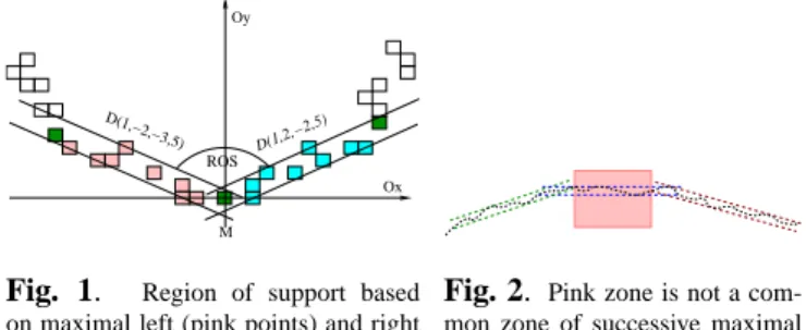
Fig. 1. Region of support based on maximal left (pink points) and right (blue points) blurred segments of M
Fig. 2. Pink zone is not a com-mon zone of successive maximal blurred segments
curve. The width of the maximal blurred segments permits to work in different scales and permits to consider the noise present in the studied curve. The width is the only parameter uses in our method. 3.1. Dominant point and region of support (ROS)
Deducing from [7], we propose in this section the notion of ROS that is compatible with the blurred segment notion.
Definition 2
Widthν maximal left and right blurred segments of a point constitute
its region of support (ROS) (see figure 1). The angle between them is called the ROS angle of this point.
Remark 1
The smaller the ROS angle of a point is, the higher the dominant character of this point is.
This remark is deduced from the work [3], where curvature at a pointCkis estimated as inverse of the radius of the circumcircle
passing throughCkand the extremities of its left and right widthν
maximal blurred segments. Therefore, we have a corollary of this remark: if the ROS angle of a point is nearly180◦, this point cannot be a dominant point.
3.2. Relation between dominant points and maximal blurred segments
In this paragraph, we study the relation between position of domi-nant points and maximal blurred segments.
Proposition 1
A dominant point of the curve must be in a common zone of succes-sive maximal blurred segments.
Proof 1
Let us consider the points on the pink zone (see Fig. 2) which are not in a common zone of successive maximal blurred segments but which belong to one blurred segment. By applying the Property 2, the left and right end points of the blurred segments of these points are also in the same blurred segment. The ROS angles of these points are nearly180◦. Therefore these points are not candidates as domi-nant points.
Let us now consider the common zone of more than 2 successive maximal blurred segments.
Proposition 2
The smallest common zone of successive widthν maximal blurred
segments whose slopes are increasing or decreasing contains a can-didate as dominant point.
Proof 2
Let us consider k successive widthν maximal blurred segments
which share the smallest common zone. Without loss of general-ity, we assume that these k maximal blurred segments do not inter-sect any other smallest zone. Suppose that there are k first maximal blurred segments with the extremities below: (B1, E1), (B2, E2),
...,(Bk, Ek). Their slopes satisfy slope1 < slope2 < ... < slopek
(similarity to decreasing case). Due to Property 1, we must have:
B1 < B2< ... < Bk;E1 < E2 < ... < Ek. Because these
max-imal blurred segments share the smallest common zone, we must haveBk< E1. So, the smallest common zone is[Bk, E1]. By
ap-plying Property 2, the left and right extremities of the points of the k partial common zones[B1, B2[, [B2, B3[, ...[Bk, E1[ respectively
are(B1, E1), (B1, E2),...(B1, Ek). The slopes of the left blurred
segments of the points of these partial common zones are always equal toslope1. On the contrary, the slopes of the right blurred
seg-ments of the points of these partial common zones respectively are
slope1,slope2, ... ,slopek. By a similar way, we deduce that on
the partial common zones]E1, E2],...,]Ek−1, Ek], the slopes of the
right blurred segments of the points of these partial common zones are equal toslopekand the slopes of the left blurred segments
re-spectively are equal toslope2, ... ,slopek. The ROS angle of the
points in the zone[Bk, E1) is equal to the angle (slope1, slopek)
and this value is minimal for all the points indexed fromB1toEk,
due to the hypothesis of the increasing slopes of maximal blurred segments. Therefore, this zone contains a candidate as dominant point.
To eliminate the weak dominant point candidates, we use the fol-lowing natural property of a maximal blurred segment, due to the shape of straight line of a maximal blurred segment and also due to the property of corner of a dominant point.
Property 3
A maximal blurred segment contains at most 2 dominant points.
3.3. Proposed algorithm
3.3.1. Algorithm
We propose below a heuristic strategy for localizing the position of each dominant point candidate. Heuristic strategy: In each smallest
common zone of successive maximal blurred segments whose slopes are increasing or decreasing, a candidate as dominant point is de-tected as middle point of this zone.
C MBS1
MBSk
Fig. 3. A dominant point is expected as center of smallest common zone.
Let us consider a small-est zone that satisfies this condition. This zone con-tains a candidate as domi-nant point (cf. proposition 2). By using the property 1, this zone must be the inter-section of the first and the last maximal blurred seg-ments in the set of succes-sive maximal blurred seg-ments that share this zone (see Fig. 3). We recall that each point in this zone has the same region of support. We then propose to lo-cate the candidate as dominant point that has geometric properties close to the expected corner point. So, the candidate as dominant
point is detected as middle point of the partial curve corresponding to this zone.
Based on the above theoretical framework and using the heuris-tic strategy above, we present hereafter our proposed algorithm for dominant point detection. It is decomposed into two parts :
• the scan of the interesting common zones of maximal blurred
segments according to the Proposition 2 and the Property 3,
• the detection of dominant points in common zones of
succes-sive maximal blurred segments whose slopes are increasing or decreasing.
Algorithm 1:Dominant point detection
Data: C discrete curve of n points, ν width of the segmentation Result: D set of extracted dominant points
begin
Build M BSν= {M BS(Bi, Ei, ν)}mi=1,{slopei}mi=1;
m= |M BSν|; p = 1; q = 1; D = ∅ ; while p≤ m do while Eq> Bpdo p+ +; Add(q, p − 1) to stack; q=p-1; while stack6= ∅ do
Take(q, p) from stack;
Decompose{slopeq, slopeq+1, ..., slopep} into monotone sequences;
Determine the last monotone sequence
{sloper, ..., slopep}; D= {D ∪ C⌊r+p 2 ⌋ } ; end 3.3.2. Complexity
The complexity of our method depends on the decomposition of a curve into maximal blurred segments that can be done in
O(n log2n) time [3]. The slope estimation of maximal blurred
segments is done in linear time. On the other hand, each maximal blurred segment is considered at most twice while the curve is de-composed into common zone of maximal blurred segments whose slopes are monotone sequence. So, in this phase, the dominant points are detected in linear time. Therefore the complexity of this method isO(n log2n).
4. EXPERIMENTAL RESULTS
The figures 4 and 5 show our obtained results and compare them with other methods (see table I) on some classical criteria: number of dominant points (nDP), compression ratio (CR), ISE error, max error, and figure of merit (FOM). CR is the ratio between number of curve points and number of detected dominant points, ISE is the sum of squared perpendicular distance of the curve points from ap-proximated polygon. As a low error of approximation leads to a low ratio of compression, Sarkar [8] propose a FOM criterion to combine these measures:F OM = CR/ISE.
Because FOM criterion is not suitable for comparation with dif-ferent dominant point number, Rosin [9] proposed other criteria to evaluate obtained result by comparing with the optimal result.
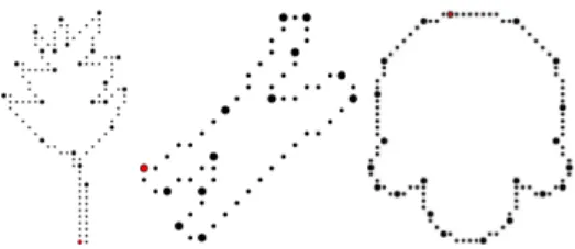
Fig. 4.Detected dominant points with default parameter (width=0.9). From left to right: leaf, chromosome, semicircle curves.
He proposed 2 measures, fidelity for error measurement and effi-ciency for compression ratio. F idelity = (Eopt/Eappr) ∗ 100,
Ef f iciency = (Nopt/Nappr) ∗ 100 where EapprandNapprare
respectively error and DP number of tested algorithm,Eoptis
er-ror of optimal algorithm with the same approximated DP num-ber, Nopt is DP number of optimal algorithm with the same
ap-proximated error. The merit measure is based on these measures.
M erit = √F idelity ∗ Efficiency. Our method is not as
effi-cient as the top 3 of the Rosin’s list [9], that contains 30 different methods (see table II), but it is better than all others.
Moreover, our method also gives good results on noisy curves as it can be seen on figure 6 and in the table hereafter. The noisy image is created by using Kanungo model [10]:
Without noise, nPoint=338 With noise, nPoint=370 width ISE CR nDP width ISE CR nDP
1 62.22 7.51 45 2 262.68 11.21 33 2 203.25 12.52 27 3 506.62 16.09 23 3 424.65 17.79 19 4 878.72 20.56 18
5. CONCLUSION
We have presented a new method for dominant point detection. This method utilizes recent results in discrete geometry to work naturally with noisy curves. The width parameter permits to take into account the noise present in the curve. For the future work, we will compare our method with other methods that can also work with noisy curves.
6. REFERENCES
[1] F. Feschet and L. Tougne, “Optimal time computation of the tangent of a discrete curve: Application to the curvature.” in DGCI, ser. LNCS, vol. 1568, 1999, pp. 31–40.
[2] I. Debled-Rennesson, F. Feschet, and J. Rouyer-Degli, “Optimal blurred segments decomposition of noisy shapes in linear time,”
Com-puters & Graphics, vol. 30, no. 1, 2006.
[3] T. P. Nguyen and I. Debled-Rennesson, “Curvature estimation in noisy curves,” in CAIP, ser. LNCS, 2007, pp. 474–481.
[4] E. Attneave, “Some informational aspects of visual perception,”
Psy-chol. Rev., vol. 61, no. 3, 1954.
[5] A. Masood, “Optimized polygonal approximation by dominant point deletion,” Pattern Recognition, vol. 41, no. 1, pp. 227–239, 2008. [6] J.-P. Reveill`es, “G´eom´etrie discr`ete, calculs en nombre entiers et
algo-rithmique,” 1991, th`ese d’´etat. Universit´e Louis Pasteur, Strasbourg. [7] C.H.Teh and R.T.Chin, “On the detection of dominant points on the
digital curves,” IEEE Trans. Pattern Anal. Mach. Intell., vol. 2, pp. 859– 872, 1989.
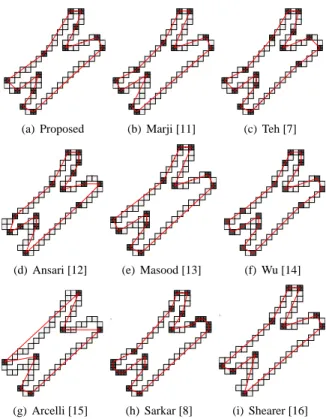
(a) Proposed (b) Marji [11] (c) Teh [7]
(d) Ansari [12] (e) Masood [13] (f) Wu [14]
(g) Arcelli [15]
y
(h) Sarkar [8]
y
(i) Shearer [16]
Fig. 5.Dominant points of the chromosome shape
[8] D. Sarkar, “A simple algorithm for detection of significant vertices for polygonal approximation of chain-coded curves,” Pattern Recognition
Letters, vol. 14, no. 12, pp. 959–964, 1993.
[9] P. L. Rosin, “Techniques for assessing polygonal approximations of curves,” IEEE Trans. Pattern Anal. Mach. Intell., vol. 19, no. 6, pp. 659–666, 1997.
[10] T. Kanungo, R. M. Haralick, H. S. Baird, W. Stuetzle, and D. Madi-gan, “Document degradation models: Parameter estimation and model validation,” in MVA, 1994, pp. 552–557.
[11] M. Marji and P. Siy, “A new algorithm for dominant points detection and polygonization of digital curves,” Pattern Recognition, vol. 36, no. 10, pp. 2239–2251, 2003.
[12] N. Ansari and K. wei Huang, “Non-parametric dominant point detec-tion,” Pattern Recognition, vol. 24, no. 9, pp. 849–862, 1991. [13] A. Masood, “Dominant point detection by reverse polygonization of
digital curves,” Image Vision Comput., vol. 26, no. 5, pp. 702–715, 2008.
[14] W.-Y. Wu, “An adaptive method for detecting dominant points,” Pattern
Recognition, vol. 36, no. 10, pp. 2231–2237, 2003.
[15] C. Arcelli and G. Ramella, “Finding contour-based abstractions of pla-nar patterns,” Pattern Recognition, vol. 26, no. 10, pp. 1563–1577, 1993.
[16] M. Shearer and J. J. Zou, “Detection of dominant points based on noise suppression and error minimisation,” in ICITA ’05, vol. 2. USA: IEEE, 2005, pp. 772–775.
Shape Algo. Nd CR M axE ISE F OM
Chro. Proposed 13 4.61 0.742 5.853 0.798 Masood [13] 12 5 0.88 7.76 0.65 Shearer [16] 10 6 6.086 0.744 Wu [14] 17 3.53 0.64 5.01 0.704 Marji [11] 11 5.45 0.895 9.96 0.548 Teh [7] 15 4.00 0.74 7.2 0.556 Ansari [12] 16 3.75 2 20.25 0.185 Arcelli [15] 7 8.57 Sharkar [8] 19 3.16 0.55 3.857 0.819 Leaf Proposed 23 5.217 0.74 11.52 0.4527 Masood [13] 23 5.217 0.74 10.61 0.49 Shearer [16] 22 5.46 13.06 0.418 Wu [14] 23 5.22 1 20.34 0.256 Marji [11] 22 5.45 0.78 13.21 0.413 Teh [7] 29 4.14 0.99 14.96 0.277 Ansari [12] 30 4.00 2.13 25.57 0.156 Arcelli [15] 16 7.50 Sarkar [8] 23 5.22 0.784 13.17 0.396 Semi. Proposed 21 4.857 0.84 10.41 0.466 Masood [13] 19 5.37 1.00 23.9 0.23 Shearer [16] 13 7.85 22.97 0.342 Wu [14] 27 3.78 0.88 9.19 0.411 Marji [11] 18 5.67 1 24.2 0.234 Teh [7] 22 4.64 1 20.61 0.225 Ansari [12] 28 3.64 1.26 17.83 0.24 Arcelli [15] 10 10.20 Sarkar [8] 19 5.37 1.474 17.37 0.309
Table 1.Comparisons using Sarkar’s criteria
Method nDP ISE Fidel. Effi. Merit Rosin’s rank Massod [13] 21 9.82 81.7 95.8 88.5 -Proposed 21 10.41 77.07 90.47 83.5 -Sarkar II [8] 20 13.65 66 78.9 72.2 4 Sarkar I [8] 19 17.38 57.8 73.7 65.3 6 Arcelli [15] 10 75.10 51.8 80.3 64.5 7 Teh [7] 22 20.61 34.0 59.2 42.4 17 Ansari [12] 28 17.83 18.8 49.1 28.8 26 Wu [14] 27 9.01 41.09 74.07 55.17
-Table 2.Comparisons using Rosin’s criteria on semicircle curve
Fig. 6. From left to rigth : First line -Leaf image, segmentations for width=2 and 3- Second line - segmentations of noisy curve [10] for width = 2,3 and 4