Probabilistic Orienteering Problem
Doctoral Dissertation submitted to the
Faculty of Informatics of the Università della Svizzera italiana in partial fulfillment of the requirements for the degree of
Doctor of Philosophy
presented by
Xiaochen Chou
under the supervision of
Prof. Luca Maria Gambardella
co-supervised by
Prof. Roberto Montemanni
Prof. Evanthia Papadopoulou Università della Svizzera italiana, Switzerland
Prof. Olaf Schenk Università della Svizzera italiana, Switzerland
Prof. Philipp Baumann Universität Bern, Switzerland
Prof. Carlo Filippi Università degli Studi di Brescia, Italy
Dissertation accepted on October 2020
Prof. Luca Maria Gambardella
Research Advisor
Università della Svizzera italiana, Switzerland
Prof. Roberto Montemanni
Research Co-Advisor
University of Modena and Reggio Emilia, Italy
Prof. Binder Walter
PhD Program Director
or in part, to qualify for any other academic award; and the content of the thesis is the result of work which has been carried out since the official commencement date of the approved re-search program.
Xiaochen Chou Lugano, October 2020
Stochastic Optimization Problems take uncertainty into account. For this reason they are in general more realistic than deterministic ones, meanwhile, more difficult to solve. The chal-lenge is both on modelling and computation aspects: exact methods usually work only for small instances, besides, there are several problems with no closed-form expression or hard-to-compute objective functions. A state-of-the-art approach for several stochastic/probabilistic vehicle routing problems is to approximate their cost using Monte Carlo sampling.
The Orienteering Problem is a routing problem aiming at selecting a subset of a given set of customers to be visited within a given time budget, so that a total revenue is maximized. Multiple stochastic variants of the problem have been studied. The Probabilistic Orienteering Problem is one of these variants, where customers will require a visit according to a certain given probability. The objective is to select a subset of customers to visit within a given time budget, so that an expected total reward is maximized while the expected travel time is minimised. The problem is NP-hard. In this work we propose different metaheuristics based on hybrid Monte Carlo sampling approximation to solve the problem. Detailed computational studies are presented, with the aim of studying the performance of the metaheuristics in terms of precision and speed, while positioning the new method within the existing literature.
In this work, we also study the use of Machine Learning tools to help solve optimization problems. By shifting the problem of selecting the number of samples used by the Monte Carlo approximation to that of choosing a trade off between speed and precision, the best number of samples can be predicted by using Machine Learning models in a fast and efficient way.
The Tourist Trip Design Problem (TTDP) is a variant of a route-planning problem for tourists interested in visiting multiple points of interest. A practical application of the POP to the prob-abilistic version of the TTDP is also discussed, and this provides inspiration for more possible applications.
I am deeply grateful to my Research Advisor Prof. Luca Maria Gambardella, Research Co-Advisor Prof. Roberto Montemanni and Academic Co-Advisor Prof. Jürgen Schmidhuber, who generously rendered help and encouragement during the process of this thesis. Whatever I have accomplished in pursuing this undertaking is due to their guidance and thoughtful advice. I would also like to thank my dissertation committee (in alphabetical order): Prof. Carlo Filippi from Università degli Studi di Brescia, Prof. Evanthia Papadopoulou from Università Della Svizzera Italiana (USI), Prof. Olaf Schenk from Università Della Svizzera Italiana (USI) and Prof. Philipp Baumann from Universität Bern. All of them have already provided valuable feedback, ideas and advice related to my research.
At this point, I would like to thank everyone who helped me through my doctoral studies culminating and contributed to my research in one way or another (again in alphabetical or-der): Aleksandar Stanic, Arpitha Bharathi, Bingrong Chen, Francesco Faccio, François Févotte, Hui Yan, Krsto Prorokovic, Mengke Ren, Micheal Wand, Murodzhon Akhmedov, Paulo Rauber, Ricardo Omar Chavez-Garcia, Robert Csordas, Thi Viet Ly Nguyen, Vasileios Papapanagiotou and Yingjie Li.
Last but not least I would like to thank my family. Thank you all for your care, support and encouragement all the time. Thank you for the wise counsel and sympathetic ear, always be there for me.
Contents ix
List of Figures xi
List of Tables xiii
1 Introduction 1
1.1 Research Motivation . . . 1
1.2 Structure of the Thesis . . . 2
1.3 Literature Review . . . 3
1.3.1 Stochastic Combinatorial Optimization Problems . . . 3
1.3.2 Machine Learning techniques in Optimization . . . 5
2 The Probabilistic Orienteering Problem 7 2.1 Problem Definition . . . 7
3 Monte Carlo sampling for the Probabilistic Orienteering Problem 11 3.1 A Monte Carlo sampling approach . . . 11
3.1.1 Methodology . . . 11
3.1.2 Experimental data sets . . . 13
3.1.3 Customers selection . . . 14
3.1.4 Tuning of the number of samples . . . 19
3.2 A heuristic speed-up criterion for the Monte Carlo sampling method . . . 20
3.2.1 Methodology of the heuristic speed-up criterion . . . 21
3.2.2 Tuning of the tolerance value y . . . . 23
3.3 Conclusions . . . 25
4 A Random Restart Local Search Heuristic Algorithm 27 4.1 A 2-opt Local Search heuristic . . . 27
4.2 Methodology of the RRLS algorithm . . . 28
4.3 Tuning of the MC evaluator embedded in the RRLS algorithm . . . 29
4.3.1 General case . . . 29
4.3.2 Tuning of the tolerance value y based on DIMENSION . . . 31
4.3.3 Tuning of the tolerance value y based on PRIZETYPE . . . 35
4.3.4 Summary and considerations . . . 37
4.4 A wiser selection of starting solutions . . . 37
4.4.1 Generation of initial solutions for the random restart phase . . . 37
4.4.2 Effectiveness of parameter k . . . . 40
4.4.3 Statistical significance of the results on parameter k . . . . 41
4.5 Conclusions . . . 43
5 A Tabu Search Heuristic Algorithm 45 5.1 The role of Monte Carlo sampling within the heuristic . . . 45
5.2 Comparison between the TS and RRLS methodologies . . . 45
5.3 Memory Structure . . . 46
5.4 Local Searches . . . 47
5.5 The Complete Tabu Search Algorithm . . . 49
5.6 Experimental Results . . . 54
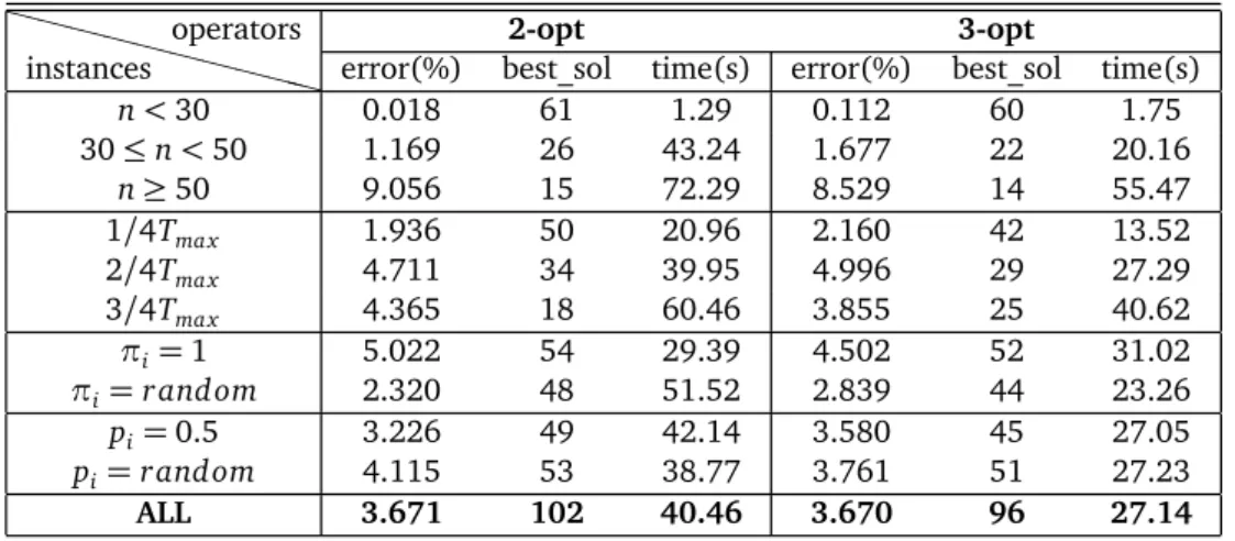
5.6.1 Random Restart Local Search TS: 2-opt and 3-opt . . . 54
5.6.2 Tuning for the length of the Tabu List: the 2-opt case . . . 55
5.6.3 Tuning for the length of the Tabu List: the 3-opt case . . . 57
5.6.4 Comparison of the TS algorithm with other methods from the literature . 60 5.6.5 Results of the TS algorithm on large instances . . . 61
5.7 Conclusions . . . 61
6 Parameters Tuning and Machine Learning 65 6.1 Introduction . . . 65
6.2 Features Selection . . . 65
6.3 Predicting the best number of samples for an instance . . . 66
6.3.1 The Concept of Satisfaction . . . 66
6.3.2 Method NN1 . . . 68 6.3.3 Method NN2 . . . 69 6.4 Computational Experiments . . . 70 6.4.1 Training . . . 71 6.4.2 Testing . . . 71 6.5 Conclusions . . . 75
7 The Probabilistic Tourist Trip Design Problem 77 7.1 Introduction . . . 77
7.2 Problem Definition . . . 77
7.3 Experimental Results . . . 78
7.3.1 Touristic application in Paris, France . . . 79
7.3.2 A comparison between the POP solvers for small instances . . . 81
7.4 Models with extra features . . . 82
7.5 Conclusions . . . 83
8 Conclusions 85
A 2-opt and 3-opt operators inside the Tabu Search algorithm: Extended Results 89
3.1 Example of s scenarios generated from a tourτ . . . 12
3.2 u(τ) of an example instance with pi= 1, πi= 0.5 . . . 15
3.3 u(τ) of an example instance with pi= 1, πi random . . . 16
3.4 u(τ) of an example instance with pirandom,πi= 0.5 . . . 17
3.5 u(τ) of an example instance with pirandom,πirandom . . . 18
3.6 Relative difference between xsand xr e f for 8 test instances . . . 20
3.7 Relative standard deviation for 8 test instances . . . 21
3.8 Computational speed for 8 test instances . . . 22
3.9 An instance with profit increase until the deadline D is incurred . . . . 23
3.10 An instance with irregular profit before the deadline D is incurred . . . . 24
4.1 Example of a 2-opt move . . . 28
4.2 Average gap (%) over time for 264 POP instances . . . 30
4.3 Analysis of Variance of the POP characteristics . . . 31
4.4 Average gap (%) over time for 84 POP instances with n< 30 . . . 32
4.5 Average gap (%) over time for 84 POP instances with 30≤ n < 50 . . . . 33
4.6 Average gap (%) over time for 96 POP instances with n≥ 50 . . . 34
4.7 Average gap (%) over time for 132 POP instances withπi= 1 . . . 35
4.8 Average gap (%) over time for 132 POP instances withπi= random . . . 36
4.9 Evolution of the best solution retrieved by RRLS over time with three initializa-tion methods (instance att48FSTCII_q1_g1_p1) . . . . 39
5.1 Comparison between the TS algorithm and the RRLS algorithm for an example instance . . . 47
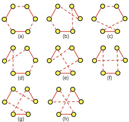
5.2 All the possible combination cases of a 3-opt move . . . 48
5.3 Converging speed of the TS algorithm on the new 24 POP instances with different dimension . . . 62
6.1 Values of speed(I, s) for different values of s for an example instance . . . 68
6.2 Values of pr ec(I, s) for different values of s for an example instance . . . 69
6.3 Values of speed(I, s), prec(I, s) and sat(I, s) for different values of s for an ex-ample instance . . . 70
6.4 Feed Forward Neural Network: Architecture NN1 . . . 71
6.5 Values of sat(I, s) for different values of s for an example instance . . . 72
6.6 Feed Forward Neural Network: Architecture NN2. The differences with respect to architecture NN1 are highlighted in red. . . 73
6.7 Distribution of the best number of samples predicted for 252 POP instances . . . 74 6.8 Satisfaction level of the prediction . . . 75 7.1 Locations of 15 Top Attractions in Paris, France . . . 80 7.2 Optimal solution for the case with equal satisfaction score for all POIs . . . 81 7.3 Optimal solution for the case with different satisfaction scores for the POIs . . . 82
3.1 The average gap increase (%) for different values v for parameter y . . . . 24
3.2 The average speed gain (%) for different values v for parameter y . . . . 25
4.1 Average gap (%) for 264 POP instances . . . 31
4.2 Detailed average error ek(%) for different k values . . . 41
4.3 Detailed p-value between k= 2 and k = 3 . . . 42
4.4 p-value over time for different k values . . . . 42
5.1 RRLS - Comparison between 3-opt and 2-opt heuristics for the POP . . . 55
5.2 Average results for the TS algorithm (2-opt) with different tabu lengths . . . 56
5.3 Best results obtained by TS algorithm (2-opt) for different tabu lengths . . . 57
5.4 Average results for the TS algorithm (3-opt) with different tabu lengths . . . 58
5.5 The 42 instances on which the 3-opt heuristic achieves more accurate results than 2-opt for the TS algorithm . . . 59
5.6 Comparison between different heuristics for the POP . . . 60
5.7 Best results found by the TS algorithm for the 24 new POP instances . . . 62
6.1 Features selected to feed the predictors . . . 66
6.2 Prediction results for the two Neural Network-based methods. Average differ-ence between the predicted value of s and the optimal one . . . . 76
7.1 List of the 15 top attractions in Paris . . . 79
7.2 Experimental comparison of heuristic methods on small instances . . . 82
A.1 TS - 2-opt vs 3-opt for 264 POP instances . . . 89
A.1 TS - 2-opt vs 3-opt for 264 POP instances (cont’d) . . . 90
A.1 TS - 2-opt vs 3-opt for 264 POP instances (cont’d) . . . 91
A.1 TS - 2-opt vs 3-opt for 264 POP instances (cont’d) . . . 92
A.1 TS - 2-opt vs 3-opt for 264 POP instances (cont’d) . . . 93
A.1 TS - 2-opt vs 3-opt for 264 POP instances (cont’d) . . . 94
A.1 TS - 2-opt vs 3-opt for 264 POP instances (cont’d) . . . 95
1 Random Restart Local Search . . . 29
2 Random Restart Local Search version 2 . . . 38
3 Random Restart Local Search (TS) . . . 50
4 Tabu Search algorithm with a 2-opt operator . . . 51
5 Tabu Search algorithm with a 3-opt operator . . . 52
Introduction
In this chapter, the motivation of the research and the contributions of our study are intro-duced, along with the structure of the thesis. A literature review on the research areas relevant to the thesis is also presented.
1.1
Research Motivation
Stochastic Combinatorial Optimization Problems have drawn the attention of many re-searchers in recent years. With respect to classic optimization approaches, uncertainty fac-tors are taken into account, thus the resulting models are more realistic. However, stochastic problems are also more difficult to solve. The challenge is both on modelling and computa-tion aspects: exact methods usually work only for small instances, besides, there are several problems with no closed-form expression or hard-to-compute objective functions. Designing efficient (meta)heuristics to produce high quality solutions in a reasonable amount of time is an actual research goal.
Metaheuristics based on (hybrid) Monte Carlo sampling have become state-of-the-art ap-proaches for several stochastic/probabilistic vehicle routing problems, such as the Probabilistic Traveling Salesman Problem (PTSP), the Probabilistic Traveling Salesman Problem with Dead-lines (PTSPD) and the Orienteering Problem with Stochastic Travel and Service Times (OPSTS). Given a problem with stochastic input data, non-stochastic constraints and an objective func-tion which is the expectafunc-tion of a certain random variable, the Monte Carlo sampling method is able to deal with different scenarios regarding the complexity of the objective function. For problems either with or without a close-form expression available for the objective function, the Monte Carlo sampling method can approximate the objective function in a fast and efficient way. Even for problems with objective functions that have already been computed efficiently, the Monte Carlo sampling method is still a strong competitor in speed and efficiency. This makes the Monte Carlo Approximation an effective evaluator to be used inside heuristic methods. In this work, we approximate the objective function of the Probabilistic Orienteering Problem by using the Monte Carlo sampling method and solve it with metaheuristic algorithms.
The Probabilistic Orienteering Problem (POP) was first introduced in Angelelli et al. [1]. It is a variant of the Orienteering Problem (OP)[63] where customers are requiring a visit with certain probabilities. In the OP, there is a set of customers at different locations and with
associated prizes. A prize is collected only if the respective customer is visited. The aim is to maximize the total prize collected within a given time budget. In the POP, the potential customers will require a visit according to given probabilities, correspondingly, a prize can be collected only when a customer actually requiring a visit is served before the given deadline. Thus, the target of the POP is to construct a planning that consists in selecting a subset of the given customers, in such a way that the respective expected prize collected is maximized and the expected total travel time cost is minimized.
Given a tour, the analytical approximation of the expected total travel time cost requires cumulative products considering all combinations in which each customer requires a visit or not. Given a feasible tour, the objective function value can be evaluated in quadratic time. However, optimizing the feasible tour is a complex task. The MILP model presented in[1] based on feasible solutions has an exponential number of constraints. The Monte Carlo sampling method is also able to approximate the objective function in polynomial time. By using it as an interrelated part of a simple local search heuristic, the POP can be solved. However, the searching process may get stuck in local extrema. We proposed a Random Restart Local Search algorithm and a Tabu Search algorithm to solve the POP. Both methods are designed to escape from local extrema and they both embed a Monte Carlo evaluator. An innovative integration of the local search heuristics and the Monte Carlo sampling method allows the creation of simple and effective algorithms. With this technique, we provide solutions for the POP with low error in a very short time.
One crucial parameter in the Monte Carlo sampling evaluator is the number of samples to be used. More samples means precision, while less samples means speed. An instance-dependent trade-off has to be found. Machine Learning techniques have been recently used in Optimization contexts. Apart from the classic experimental tests, we are also interested in understanding whether a Machine Learning model can effectively predict the number of samples required for an instance or not. Two methods are presented and compared from an experimental point of view. It is shown that a less intuitive and slightly more complex method is able to provide more precise estimations.
Finally, we are also interested in the possible application of the POP. The Touristic Trip Design Problem (TTDP) is a variant of a classic route-planning problem for tourists interested in visiting multiple points of interest. A simple formulation of the TTDP is proven to be identical with the OP. Adhering to the practicality, we also take uncertainties into consideration for the TTDP. In fact, a variety of uncertainties could affect the availability of the points of interest. For example, popular places may probabilistically require a long waiting time and open-air places may not be visitable due to unseasonable weather. In this work, we define the Probabilistic Tourist Trip Design Problem (PTTDP) and show that simple POP solvers can efficiently provide solutions for this application.
1.2
Structure of the Thesis
The structure of the document is as follows.A review of the literature focusing on the POP and on common methods used for several related stochastic combinatorial problems is presented in Section 1.3. In Chapter 2, a detailed formal definition of the problem studied is provided. A Monte Carlo evaluator is presented in
Chapter 3. The Monte Carlo evaluator is then embedded in a Random Restart Local Search algorithm presented in Chapter 4 to solve the POP. In Chapter 5, we describe a Tabu Search algorithm based on the Monte Carlo evaluator as well. Experimental tests on the performance of the metaheuristic algorithms proposed are carried out in both Chapters, with an analysis of limitation and advantages of the approach with respect to other methods from the literature. In Chapter 6 we discuss the use of Machine Learning technologies for parameter tuning purposes. In Chapter 7 a stochastic Tourist Trip Design Problem with personalized customisation is pre-sented and solved by using the methods proposed in the previous chapters. Finally, conclusions are drawn in Chapter 8.
1.3
Literature Review
In this section, we give an overview about publications regarding stochastic combinatorial problems related to our research, technical aspects of the Monte Carlo sampling methods, the metaheuristics using the Monte Carlo sampling approximation of the objective function, and the use of Machine Learning techniques in Optimization contexts.
1.3.1
Stochastic Combinatorial Optimization Problems
The Probabilistic Orienteering Problem (POP) was first introduced by Angelelli et al. [1]. It is a variant of the Orienteering Problem (OP) where customers are requiring a visit with certain probabilities. Detailed information of the OP along with survey can by found in Vansteenwegen et al.[63] and Gunawan et al. [27].
As shown in Feillet et al.[5] and Bérubé et al. [21], the OP can be formulated as a Travelling Salesman Problem with Profits. The problem has been proven to be NP-hard by Golden et al. [26]. To solve the OP, a brand-and-bound method is used by Laporte and Matello [38] and Ramesh et al. [50]. Improved approaches based on branch-and-cut have been proposed by Fischetti et al. [22] and Gendreau et al. [24]. There have been continuous improvements to the solving methods over the years, and a classification of the exact algorithms and details about the applied techniques can be found in Feillet et al.[21]. The OP arises in several real domains. A recent application is the Mobile Tourist Guide introduced in Souffri et al.[56], which makes feasible plan for tourists to visit the most valuable attractions among all the places that they wish to visit in the limited time of the trip. Such planning problems are called Tourist Trip Design Problems (TTDP) (Vansteenwegen and Van Oudheusden[60]). Similar Tourist Trip problems of selecting the most interesting combination of attractions is mentioned in Chou et al. [18] and Wang et al.[66]. In general, the application of the TTDP requires high quality solutions in a short calculation time, which helps to make real-time decisions.
There are several deterministic extensions to the OP. The Team Orienteering Problem (TOP) [12, 59, 3] considers multiple routes limited by the deadline and the goal is to maximise the total prize collected. The Orienteering Problem with Time Windows (OPTW) and the Team Orien-teering Problem with Time Windows (TOPTW) add time window constraints for the customers, and a visit to a customer can only starts during this time window. The OPTW and TOPTW have been solved with Ant Colony optimization by Montemanni and Gambardella[46, 47], and It-erated Local Search metaheuristic by Vansteenwegen et al.[62]. Another interesting variation of the OP is the Clustered Orienteering Problem (COP) proposed by Angelelli et al.[2], where
each profit is associated with a cluster of customers and is gained only when all customers in the cluster are served.
The probabilistic variations of the OP are mainly considering uncertainty on time and/or profit. From the objective perspective, the POP we study in this work is similar to the Proba-bilistic Travelling Salesman Problem with deadline (PTSPD)[11]. In the PTSPD, a minimum expected cost a priori tour is to be find through a set of customers with probabilities of requiring service. Each customer has a deadline, and service at each customer should begin at or before its deadline. The objective is to minimize the expected travel time and the expected penalty caused by violation of the deadline. In Campbell et al. [11], different models are considered such as paying a penalty for any violation of a deadline, or paying penalties for skipping the customers whose deadline would be violated. In both the POP and the PTSPD, the stochas-ticity is on the probability of a customer requiring service. The main difference is that in a POP feasible solution every customer on the tour must be visited before the global deadline, while in PTSPD customers can be visited after the deadline, paying a penalty. Other variants of the OP with stochasticity on service or travel time have been studied in Tang and Miller-Hooks [58] and Campbell et al. [10]. A vehicle routing problem with stochastic travel times and soft time windows is considered in Russel and Urban[52]. An OP with uncertain prizes has been considered in Ilhan et al. [33]. From an application perspective, a tourism-related practical application of the POP has been studied in[18].
The basic models can be extended with extra feature. For example, a Probabilistic Team Orienteering Problem (PTOP) based on the Team Orienteering Problem (TOP) is discussed in Chao et al.[12] and Tang and Miller-Hooks [59]. The PTOP can be open to more applications, such as planning a different tour for each day during the length of the stay, or determine same or separate tours for a tour group, regarding the different satisfaction scores given by each member in the group and the availability of the points of interests on the list. A much further probabilistic extension of the problem can also be based on the variations of the OP, such as OPTW and TOPTW.
The POP inherits the NP-hardness from the OP[1]. To solve the POP, a MILP model has been proposed and the problem is solved by branch-and-cut methods in Angelelli et al. [1]. Since solving with a basic branch-and-cut method is computationally demanding, three matheurstic methods to reduce the solution time (detailed in Section 3.1.2) have also been also studied in [1]. The use of Monte Carlo sampling techniques in the context of the POP has been studied in Chou et al. [14]. A fast objective function cost approximator for the problem using Monte Carlo sampling method has been proposed. Similar uses of the Monte Carlo sampling approach for stochastic/probabilistic vehicle routing problems can be found in Weyland et al. [67] and Papapanagiotou et al.[48]. Given the characteristics of an instance, a Machine Learning-based study on estimating the best number of samples to use in such a Monte Carlo sampling evaluator for the POP can be found in Montemanni et al.[45].
Local search methods provide fast and efficient heuristic solutions for problems with high computational complexity[30]. For example, the 2-opt heuristic ([19, 23, 40, 34]) is proven to be crucial to obtain high quality results for the TSP and OP. However, a standard technique like 2-opt and 3-opt[6] which only searches in the neighborhood of the solution may get trapped in local extrema[54]. To take care of this undesired phenomenon, random restart strategies applied on top of the local search adopted are normally used, in order to increase the probability of success in searching procedures. The method works by restarting the optimization search
once no further improvement is possible by the embedded local search component. In our work, a solver with heuristic speedup criterion for the POP (details in Chapter 4) using Random Restart mechanism is proposed, which proved to be fast and efficient for small instances problems. A study on improving the performance of the solver by modifying the generation of re-initialising solutions is also presented in[17].
Tabu Search (TS) is a metaheuristic search technique that has been widely used in combi-natorial optimization problems since it was introduced by Glover[25]. It is another effective method to deal with local extrema. The basic idea is to accept a sequence of non-improving solutions to escape from local extrema. This is achieved by the use of an explicit memory called Tabu List during the search process. It avoids visiting solutions that have been visited recently. A variety of implementations of Tabu Search in the context of the Travelling Salesman Prob-lem and related probProb-lems is reviewed and compared in Basu[4]. Other methods have been proposed, such as Simulated Annealing in Kirkpatrick et al. [35], Genetic Algorithms in Hol-land[29] and Ant Colony Optimization in Dorigo and Gambardella [20]. They are other tech-niques frequently used to escape from local extrema. The Tabu Search method implemented by Kulteral-Konak et al. [37] has been compared with a Multi-Level Variable Neighbourhood Search (MLVNS) algorithm on solving large OP instances in Liang et al.[39]. In the MLVNS, in-stances with identical settings (i.e. dimension, coordinates, and associated scores of the nodes) differing only in the constraint levels will be solved concurrently. In this way, information from the searching process can be shared among the instances to improve the efficiency. Experimen-tal results show that the MLVNS performances better on the quality of the solutions, while the TS requires shorter computing time.
1.3.2
Machine Learning techniques in Optimization
Machine Learning techniques have been recently used in Optimization domain. Examples of such methods can be found in the context of branch and bound solvers for Mixed Integer Programming: the branching strategy has a key role in the performance of methods. In Hutter et al.[31] some methods are devised to learn which is the best strategy. The idea is to identify some features of the present sub-problems or the present search-tree node, based on which the branching strategy to employ is selected, in order to mimic in a fast way the so-called strong branching that guarantees the best performance, but is time-consuming [42]. The training phase of the neural network can either be done before or during the run of the branch-and-bound algorithm. A successful combination of Monte Carlo Tree Search and Deep Learning can be found in Silver et al.[55] and Parascandolo et al. [49].
Another trend is to use Machine Learning techniques to tune the parameters of the solving methods such as in Calvet et al. [9], Hutter et al. [32], and Lodi et Zarpellon [41]. Such methods again rely on the identification of some features and as it was happening with the previous application the identification of such features is very crucial for the performance of the methods. A similar application, based on a similar concept of features identification and evaluation, is to adopt Machine Learning techniques to forecast the running time of an algorithm ([32]) or classifying quadratic programming problems in terms of the best algorithm to use to solve them[41]. The use of Artificial Neural Networks in Optimization has been considered in Villarrubia et al. [65]. Another Machine Learning-based study on Reinforcement Learning for the Travelling Salesman Problem is discussed in Mele et al. [44].
The Probabilistic Orienteering Problem
2.1
Problem Definition
The Probabilistic Orienteering Problem answers the following question: given a time budget and a list of customers at different locations with different probabilities of requiring a visit and deterministic prizes to be collected, what is the best subset of customers to visit (and in which order) so that the expected total collected prize is maximized and the travel time is concur-rently minimized? This problem, faced by companies while organising their day-ahead plan or general users having to take real time decisions[18], is a variation of the Orienteering Problem which takes uncertainties of the customers’ requirements into consideration, with uncertainty modelled through probabilities.
As described in[63], the Orienteering Problem can be defined on a graph G = (V, A) where V = {0, 1...n, n + 1} is the node set representing customers with the depot being node 0 and the destination being node n+ 1 and A is the arc set representing the paths between pairs of customers. A prize pi is associated with each node, a travel time ti j is associated with each
arc ai j ∈ A and a deadline D is finally provided. A feasible tour σ is defined as a sequence
of customers that can be visited before the deadline incurs. With this notation, the OP can be described as the problem of finding the tour that collect the largest possible amount of prizes from customers within the given deadline[63]. This of course implies a selection of the shortest tour among the selected customers. The objective function of the OP can be reduced therefore to the maximization of the following quantity o(σ), given a feasible (partial) tour σ not exceeding the deadline D:
o(σ) =X
i∈σ
pi (2.1)
Differently from the OP, the objective function of the POP is no longer a simple sum. Due to the probabilistic nature of the problem, customers that offers a large prize may require a visit with a very low probability. With this consideration, the POP is defined as follows.
A POP instance contains the information(V, t, π, D, p) where:
• V = {0, 1...n, n + 1} is the set of n customers (nodes) with the depot being node 0 and the destination being node n+ 1.
• D is the global deadline.
• ti jis the deterministic travelling time from customer i to customer j defined, for all i, j∈
V.
• πiis the probability of a customer i∈ V to require a visit and is modeled in our study by
a Bernoulli variable bi= {0, 1}. bi takes value 1 with an independent probabilityπifor
each customer. Depot and destination are required to be visited by definition, therefore πo= πn+1= 1.
• piis the prize collected when a customer i ∈ V is served before the global deadline D.
There is no prize for depot and destination, therefore p0= pn+1= 0.
Formally, we define a feasible solutionσ = (i0= 0, i1, i2, ..., iq, iq+1= n+1) as a tour starting from the depot, allowing to serve a sequence of q customers even when all customers on the route require visits and going to the destination before the global deadline D. A complete tour τ = (0 = i0, i1, i2, ..., in, in+1= n + 1) is defined as a sequence of n customers, plus the depot
and the destination node. For a given complete tourτ, the associated prize is P(τ) and the associated travel time is T(τ).
The POP is a combinatorial optimization problem with the objective of maximizing the total expected prizes collected while visiting customers before the given deadline, minus a measure of the total expected travel time. The last factor helps to make a choice when several tours are associated with a same total prize, and in this case we pick the one associated with smaller travel cost. Note that the travel time component is not present in the classic formulation of the OP described above.
The objective function of the POP is to retrieve a feasible solutionσ among all possible tours that maximize the following quantity:
u(σ) = E[P(σ)] − C E[T(σ)] (2.2)
where the difference between the expected total prize and the expected total travel time is multiplied by a given coefficient C that is normally set by the decision maker[1].
From a computational perspective, solving the POP is computationally demanding. Given a feasible tour, the objective function value can be evaluated in quadratic time by using the following formulas ([1]): E[P(σ)] = q X k=1 πkpk (2.3) E[T(σ)] = q X h=0 [πh q+1 X k=h+1 (thk· πk· k−1 Y j=h+1 (1 − πj))] (2.4)
where it is assumed thatQkj=h+1−1 (1 − πj) = 1 whenever h + 1 > k − 1.
However, optimizing the feasible tour is a complex task. The MILP model presented in[1] based on feasible solutions has an exponential number of constraints.
The main purpose of our study is to design simple heuristics to solve the POP in a simple and effective fashion. To achieve this, we think from another perspective to work with complete tours directly generated from the POP instances. The best complete tour can be easily obtained
by local search heuristics, and the best feasible solution can be extracted from the best complete tour. In this way, the bottlenecks are transferred to the evaluating part in our approach. We design a smart Monte Carlo evaluator. It not only evaluates the objective function value of a given complete tour, but also extracts the best feasible solution out of the given tour with the maximum profit, which is consistent with the objective function, during the evaluation. In this way, when two complete tours are associated with a same feasible solution, the evaluator is be able to tell the difference within the local search procedure, and picks the one that is more likely to lead to a better searching space and eventually improves the accuracy of the solving method. The smart Monte Carlo evaluator is described in the following Chapter 3, and it is used as an interrelated part of heuristics we propose (see Chapter 4 and Chapter 5)) to solve the POP eventually.
Monte Carlo sampling for the
Probabilistic Orienteering Problem
3.1
A Monte Carlo sampling approach
In this section we propose a way of evaluating the objective function value of the Proba-bilistic Orienteering Problem described in Chapter 2 by using a Monte Carlo sampling method. The work presented has appeared in[14].
3.1.1
Methodology
The objective function value is approximated by the Monte Carlo sampling method (MC) in the following way: for a given complete tourτ with n customers, according to the probability of each customer to require a visit, a set of s deterministic scenarios is generated. Each scenario is a fully connected graph with a fixed set of customers requiring a visit and implies therefore a tourτJ obtained byτ by cancelling the customers not present in scenario J. For each scenario
J∈ {1 . . . s}, a deterministic objective function value can be evaluated in linear time as ud(τJ) = P(τJ) − C · T(τJ), thus the objective function value u(τ) of the tour τ can be approximated by averaging these values in time O(ns).
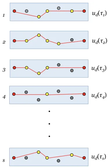
Figure 3.1 shows an example of generating s scenarios for a given complete tour τ = (0, 1, 2, 3, 4, 5, 6), with 0 being the depot and 6 being the destination. Each block represents a scenario and each dot in the block represents a node, which can be either a customer or the depot/destination. In each scenario, whether a customer requires a visit (yellow) or not (grey) is deterministic. When a customer i does not require a visit, he will be skipped while travelling on the tourτ, and the truck moves from the previous customer directly to the next customer that requires a visit. For example in scenario 1, customer 1 and 4 do not require a visit, there-fore, a tourτ1= (0, 2, 3, 5, 6) is obtained, and straightforwardly, its objective function value ud(τ1) can be calculated. Similarly, a total of s scenarios are generated regarding the probabil-ity of each customer in tourτ requires a visit. With ud(τJ) being the deterministic cost of the
tourτJ adapted to the deterministic scenario J , the approximation value for u(τ) is given by
Figure 3.1. Example ofs scenarios generated from a tourτ
the average objective function value of the deterministic costs of all the scenarios considered:
u(τ) ≈ s P J=1 ud(τJ) s (3.1)
By design, our solver treats complete tours touching all customers, while a feasible solution only visits a subset of customers that can be served before the deadline D. Thus the Monte Carlo evaluator is also delegated to extract a feasible solutionσ(τ) as a prefix of a complete tourτ.
By the definition of the problem, the travel time of going from the last visited customer back to the depot has always to be considered. Due to this feature, when a complete tour τ = (i0= 0, i1, i2, ..., in, in+1= n + 1) is being evaluated over a given deterministic scenario s,
the tour stops at the last customer iq(q ≤ n) before the deadline D is incurred, and then goes
directly to the destination node. The best feasible POP solution selected out of a complete tour can also be easily obtained in this way by supposing all customers on the route require visits. However in certain situation, it is possible that some customers visited within the deadline are not offering enough prize to make an increase on profit. Therefore, to make a smarter selection that is consistent with the objective function, we take the best feasible solutionσ(τ) selected out of a complete tourτ as the one with the peak value of (3.1) encountered during the evaluation ofτ, denoted as u(σ(τ)). This coincide with the fact that during the evaluation of a complete tourτ, after the deadline is incurred only the travel time component increases, but no more prize is collected.
Experimental examples on customer selection regarding this peak value during evaluation can be found in Section 3.1.3. A detailed design choice for the heuristic speed-up criterion with parameters tuning is presented in Section 3.2, where the Monte Carlo evaluator is able to un-derstand how to cut the best feasible solutions from given complete tours, and stops evaluating at proper time to improve the speed of the evaluation while not losing precision.
In conclusion, the Monte Carlo Approximation component receives in input a (complete) tourτ and outputs:
• a POP feasible solutionσ(τ) extracted from the complete tour τ;
• an approximation for the objective function value u(τ) of the complete tour τ; • an approximation for the objective function value u(σ(τ)) of the POP solution σ(τ). Due to the heuristic nature of the approach, the approximation of the objective function value is more accurate when more scenarios are used, but this requires more computational time. In the following subsections, experiments are carried out to understand which could be promising values for the number of samples to be used for evaluation.
3.1.2
Experimental data sets
The POP benchmark instances used for the main experiments in this work are the 264 in-stances introduced in[1]1. They are based on 22 TSP benchmark instances from the TSPLIB95 library2 [51]. With reference to the definition in Section 2.1, the characteristics of the POP instances are set as follows:
• The customers information and distances are taken directly from the corresponding orig-inal TSP instances. The first customer of the origorig-inal instance is considered as the depot. The destination vertex coincides with the depot.
• The global Deadline D takes value ofω · Tma x, with Tma xbeing the known optimal value
of the original TSP instance and ω = {14,12,34} representing short, medium and long deadlines.
• The probabilities of the customers to require visits are eitherπi= 0.5 for all customers,
orπiis a random number in the interval[0.25, 0.75] for each customer i.
• The prizes collected while visiting the customers are either pi= 1 for all customers, or pi
is a pseudo-randomly generated integer in{1, 2, ..., 100} for each customer i. 1The POP instances are available at http://or-brescia.unibs.it/instances
The coefficient C of the objective function (2.2) used to balance between the travel times and the prizes components is taken as C= 0.001, in order to maintain full compatibility and comparability with the results of[1], where the same setting is considered.
The testing environment is a computer equipped with a Quad-Core Intel Core i7 processor 2.0 GHz (only one core is used for the experiment) and 8GB of RAM. The Monte Carlo evaluator was implemented in C++. These settings are used for all the experiments reported in this Chapter.
3.1.3
Customers selection
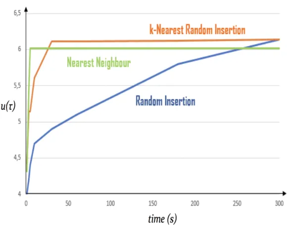
As mentioned in Section 3.1.1, the Monte Carlo evaluator is able to extract the best feasible solution out of a given complete tour during evaluation. Instead of using simple strategies such as calculating the average of maximum number of customers served before the deadline, we calculate the value of objective function for each node with all samples, supposing that it is the last customer visited. In such a way, by arriving at each customer on the tour, there is an objective function value of the corresponding feasible solution. The peak value will show the best feasible solution that can be extracted from the given complete tour. The approach is heuristic but it provides good results in practice.
First, we test the idea on two instances with the same location information and prize values, but different probability types of requiring a visit. In this two instances, the prize pi= 1, ∀i ∈ V ,
and the probabilityπiof requiring a visit is either fixed with value 0.5 or random. The results
are plotted in Figure 3.2 and Figure 3.3, where the x-axis shows all nodes{0, 1...n} in the order of a given solution, and the y-axis shows the approximated value for the objective function at each node, as described in Section 3.1.1.
From the results in Figure 3.2 and Figure 3.3 we can observe that, given two instances with the same location information and prize values, the slopes of the evolution of the objective function value are similar for both instances with random and fixed probability of requiring a visit. In both cases there exists a significant maximum at node 14 showing the best node to stop serving customers.
Then we try on two instances still with the same location values, but with random prize pi
for each customer. The probabilityπi of requiring a visit is still either fixed with value 0.5 or
random. The results are plotted in Figure 3.4 and Figure 3.5. This time total prize collected at local maximum has much higher value than in Figure 3.2 and 3.3, but the travel time after the local maximum is increasing as in the previous experiments. Therefore the curve is almost flat after the local maximum. A maximum can however be observed, showing again the best stopping point.
By inspecting the curves, the best feasible solution of a given complete tourτ can be ex-tracted during the evaluation process. Therefore the idea provides an heuristic idea to perform the evaluation only on the subset of customers of the best feasible solution. This will speed up the evaluation and lead to more accurate results within appropriately designed heuristic solvers, since an external tool to select the customers to visit is not required. Further discussion on how to detect the peak value without evaluating until the end of the tour can be found in Section 3.2.
3.1.4
Tuning of the number of samples
In this part, we study the influence of number of samples s when approximating the objective functions using Monte Carlo sampling.
In the experiments, the Monte Carlo evaluator is run 50 times on the solutions of 8 different POP instances, with different number of samples s ∈ {10, 20, ... , 90, 100, 200, ... 1000}. Given a solution, we compute xsas the average value of the objective function approximated
with s samples. Since an exact solution is not available for all the instances considered, the best (feasible) solution and the corresponding objective function value reported in[1] for each instance is considered as a reference value Xr e f.
Two indicators are set for the analysis of the results on each instance. δ1 is the relative difference between xs and xr e f, which indicates the accuracy of the results. δ2 is relative standard deviation for each number of sample s, which indicates the stability and consistency. The indicators are calculated as follows:
δ1= xs− xr e f · 100 xs (3.2) δ2= v u t P50 i=1(xi− xs)2 N · 100 xs (3.3)
Notice: Both indicators are calculated with the relative values instead of absolute values, in such a way that the results obtained on different instances can be compared together for more general conclusions.
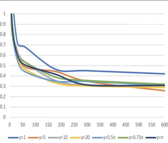
Figures 3.6 and 3.7 show the values of indicatorδ1andδ2on the y-axis, for the different number of samples s on the x-axis. Each curve represents a test instance of the 8 considered. In Figure 3.6 we can observe that generallyδ1 reduce to 1% when s≥ 50, but δ2in Figure 3.7 is still relatively high around s= 50. Considering δ1andδ2together, if a small number of samples is wanted for the experiments, 50 could be the choice, while considering stability of the results, 400 is a better choice. It is worth noting that, in a more instance-dependent analysis, for some instances, values of s lower than 50 work well, for others higher values are needed. Therefore, the choice of the number of samples can be instance dependent.
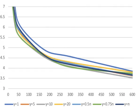
We are also interested in the computing speed as a function of the number of samples. We remind the reader that the theoretical computational time for the evaluation of a solution is O(ns), where n is the dimension of an instance and s the number of samples. The computation time is longer for instances with larger dimension and when more samples are used for evalu-ation. However in practice, the evaluation is extremely fast. Therefore, we use the number of evaluations per second instead of computation time for a more meaningful observation. Fig-ure 3.8 shows the number of evaluations per second on the y-axis, for the different number of samples s on the x-axis. Each curve represents a test instance among the 8 considered. With t being the actual computation time, the number of evaluation per second represents the value of 1t.
Theoretically, the computation time t increases linearly with increasing s, while the number of evaluations per second decreases gradually as a consequence. In Figure 3.8 we observe the same: for s ≤ 100, the number of evaluations per second drops dramatically when s is
Figure 3.6. Relative difference between xs and xr e f for 8 test instances
increased, while for s > 100 there is a trend of a more gradual decrease. The size of the instances n influences the computational speed as well as mentioned.
In general, the relative difference between xsand xr e f is less than 1% when s≥ 50 according
to Figure 3.6, and the computational speed is over 105evaluations per second when s≤ 250 according to Figure 3.8. Therefore, number of samples 50≤ s ≤ 250 is a considerable choice to be used for the Monte Carlo sampling method which gives a good balance between the quality of the approximation and the computation speed.
More in general, we can conclude that Monte Carlo sampling is an extremely fast and precise method, and appears to be suitable to be used inside heuristic solvers.
3.2
A heuristic speed-up criterion for the Monte Carlo sampling
method
In Section 3.1 we have proven the Monte Carlo sampling approximation is fast and efficient to be used for evaluating the objective function of the POP. In this section we build a Monte Carlo evaluator with a heuristic speed-up criterion based on the characteristics of the POP, which offers the possibility of further improvements on evaluating speed. The work presented has appeared
Figure 3.7. Relative standard deviation for 8 test instances
in[15].
3.2.1
Methodology of the heuristic speed-up criterion
By design, when the Monte Carlo evaluator is embedded in heuristic solvers for the POP (see Chapter 4 and Chapter 5), complete tours including all customers from the input instances are fed directly to the evaluator. As mentioned in Section 3.1.3, during the evaluation of a complete tourτ, a peak objective function value will be encountered, and only the customers visited until this peak are selected for a visit. Therefore, a heuristic approach could be used to identify this last customer visited at the peak value and stop the evaluation of the remaining customers. Since finding this maximum value is consistent with the objective of the POP, by stopping the evaluation after the deadline is incurred, unnecessary calculations will be avoided and the computation time can be reduced.
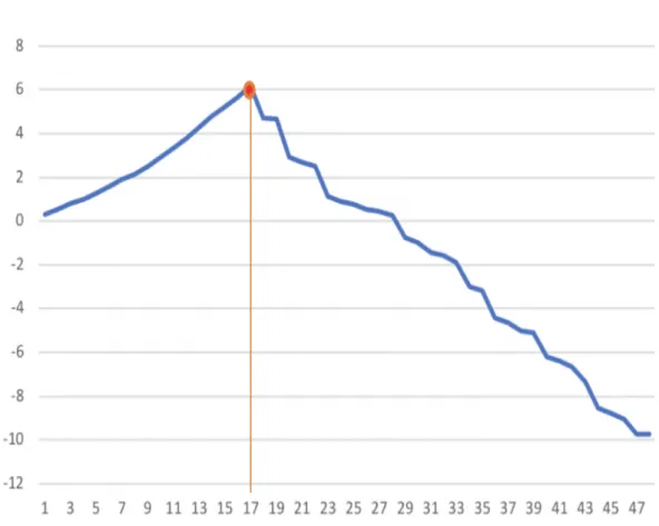
Ideally, the objective function value increases when we visit one customer after another, and the maximum value is obtained at the last node visited before the deadline D (Figure 3.9). This fits the usual situation encountered in real life problems: the customers of the sequence are visited with a positive profit until the deadline is incurred. At this point, a maximum value can be observed, and after that it is not worth to continue the tour because the balance only decreases due to the extra travel time incurred without picking up any prize.
Figure 3.8. Computational speed for 8 test instances
However, the profit of the POP is the difference between the expected prize and expected travel time, and this subtraction causes an issue: we cannot guarantee a positive profit for all customers visited before the deadline, especially for instances in which customers are far away from each other and each of them has a relatively low prize associated. In such a case, a few customers might be visited with negative profit before the deadline incurred, thus the heuristic speed-up criterion cannot simply stop the evaluation once the first drop in the expected profit is detected by the Monte Carlo evaluator (Figure 3.10). To deal with this problem, a tolerance value y that allows the profit to drop several times is introduced to prevent the evaluation from stopping too early due to a temporary negative profit, while not wasting time to evaluate the whole tour anyway. With an appropriate value of y, the accuracy of the best feasible solution extracted during evaluation can also be improved, by excluding the circumstances when the travel time still allows to visit a few more customers before the deadline, but the prizes collected are not enough to make an increase of profit.
When y=1, the evaluation stops when the objective function value first starts to decrease. This would save the most time for the instance in Figure 3.9 but will severely affect the ap-proximation accuracy for the instance in Figure 3.10. If y takes the value of the dimension n of a given instance, the evaluator always computes until the last node without stopping (and returns the maximum value and the corresponding position for the best feasible solution). This is equivalent to the case where the heuristic speed-up criterion is not implemented, thus no
Figure 3.9. An instance with profit increase until the deadlineD is incurred
speed is gained, and no accuracy is lost.
In the following subsection, we study on the impact of the heuristic speed-up criterion in terms of precision and speed.
3.2.2
Tuning of the tolerance value
y
With the same data sets and testing environment described in Section 3.1.2, experiments are run for each instance of the 264 POP instances with the number of samples set to s= 100. As alternatives for the parameter y, four fixed values {1, 5, 10, 20} and four flexible values {1/10n, 1/4n, 1/2n, 3/4n} are tested, with n being the number of customers of the instance under investigation. The solutions considered for these tests are the best known solutions avail-able for each instance.
We denote as Xvthe evaluation value of a complete tour obtained by the Monte Carlo
eval-uator with a certain value v for parameter y. The value Xnobtained with v= n is considered
as a baseline. The gap for a given value v for parameter y is calculated as follows:
g ap(v) = |Xv− Xn| ·100 Xn
Figure 3.10. An instance with irregular profit before the deadline D is incurred Table 3.1. The average gap increase (%) for different values v for parameter y
Fixed v 1 5 10 20
g ap(v) 8.627 0.321 0.005 0
Flexible v 0.1n 0.25n 0.5n 0.75n
g ap(v) 0.408 0 0 0
We calculate the average gap for the 264 instances in Table 3.1.
From Table 3.1 we can observe that when v= 1, the evaluation has a relatively large gap in average, which shows the negative profit situation described in Figure 3.10 exists among the 264 test instances considered. The gap goes down as v increases, and there is no gap between Xvand Xnwhen v≥ 20 or v ≥ 0.25n.
We then consider the average computation speed for different v value. We again consider the computation speed with v= n as a baseline Sn and the average computation speed with
a certain v value is denoted as Sv. The average speed gained with different values of v for
parameter y is calculated as follows:
speed gain(v) = |Sv− Sn| ·
100 Sn
Table 3.2. The average speed gain (%) for different values v for parameter y
Fixed v 1 5 10 20
speed gain(v) 8.9 7.5 5.3 2.1
Flexible v 0.1n 0.25n 0.5n 0.75n speed gained(v) 6.6 5.3 3.3 0.03
We calculate the average speed gained with different v values for each instance, then com-pute the average speed gained for all the 264 instances in Table 3.2.
From Table 3.2 we can observe that the speed is improved by 8.9% when we take v= 1. The speed decreases when v takes larger values. When the value reaches v= 0.75n, the speed-up effect is negligible.
From the Monte Carlo evaluator perspective, we conclude that v= 0.25n or v = 10 are good choice for general case. Note that when the Monte Carlo evaluator with speed-up criterion is embedded into a solver (see the RRLS solver in Chapter 4), the value of tolerance y influences as well the search path, which may lead to different solutions. Therefore, the choice for the value of tolerance y could be peculiar in different solvers.
3.3
Conclusions
In this chapter we introduced a method of approximating the objective function of the Prob-abilistic Orienteering Problem based on Monte Carlo sampling. The same Monte Carlo sampling procedure is used to decide how many customers of a given complete tour should be visited in order to maximize the profit, and a relevant best feasible solution is extracted. Such a novel characteristic is going to be very useful once the evaluator is embedded into metaheuristic al-gorithms introduced in the coming chapters. Computational studies on the performance of the Monte Carlo evaluator with a speed-up criterion we introduced, both in terms of precision and speed, were also presented.
A Random Restart Local Search
Heuristic Algorithm
In Chapter 3 we have discussed the use of Monte Carlo sampling method for the approxi-mation of the objective function value of the Probabilistic Orienteering Problem. Our purpose is to use the Monte Carlo evaluator described in Section 3.2 as interrelated part of heuristic methods to solve the problem. In this chapter, a POP heuristic solver based on the embedding of the Monte Carlo evaluator in a Random Restart Local Search heuristic is proposed. The work has appeared in[15]. A study on different methods of (re-)initialising solutions to improve the performance of the algorithm is also discussed. This related work has appeared in[17].
4.1
A 2-opt Local Search heuristic
In the searching process of an optimization algorithm, we move from one complete tour to another based on the concept of neighbourhood of a given tour. The neighbourhood is defined by a local search method. By combining the local search method and the Monte Carlo evaluator we propose, a POP solver is designed.
The first local search method we use in this work is a 2-opt heuristic proposed by Croes[19] with basic move suggested by Flood[23], which deletes two non-adjacent edges of a tour and reconnects the two paths resulting from this break in the other possible way without creating sub-tours. To be more specific, for a given tourτ = (i0= 0, i1, i2, ..., in, in+1), we pick all possible first customer j from{i1, ..., in−1} and all possible second customer k from {ij+1, ..., in}, then
reverse the path between these two customers, obtainingτ0= (i0, i1, ..., ij, ik, ik−1, ..., ij+1, ik+1,
..., in, in+1). A corresponding example of the 2-opt move is shown in Figure 4.1. More details
on the 2-opt heuristic can be found in[34]. The sequence of the new tours generated from τ is referred to as the neighborhood ofτ, and is denoted as N (τ).
Some theoretical results about the number of complete tours and feasible solutions present in the 2-opt neighbours are considered, which help to understand the searching process more intuitively, especially when metaheuristics are built on top of the local search procedure (for example, the Tabu Search heuristic presented in Chapter 5).
Given a complete tourτ with n customers, the total number of complete tours contained 27
Figure 4.1. Example of a 2-opt move
in the 2-opt neighbourhood N(τ) is determined by the number of combinations of picking 2 customers out of n:
|N (τ)| =n(n − 1)
2 (4.1)
Given a feasible solutionσ(τ), the total number of feasible solutions contained in the 2-opt neighbourhood N(σ(τ)) is determined by the number of combinations of picking 2 customers out of q, with q= |σ(τ)| being the number of customers in the feasible solution σ(τ) extracted from the complete tourτ:
|N (σ(τ))| =q(q − 1)
2 (4.2)
4.2
Methodology of the RRLS algorithm
The method starts with a complete tourτ0generated at random. The tour is then optimized by crossing over with a 2-opt heuristic operator that iteratively deletes two edges of a first-improve tour and reconnects the two paths resulting from this break in the other possible way (as described in Section 4.1). The evaluation of each tour is done by the Monte Carlo sampling approximation (see Section 3.2), that evaluates the objective function value u(τ) of a given tour τ, as well as deciding the subset of customers to serve, by extracting the best feasible solution σ(τ) with the objective function value u(σ(τ)). The current best tour τl ocalis updated every
time a better tour is found in the neighborhood N(τ) generated by the 2-opt method, and a new sequence of swaps is generated from the current best tour. When no improving tour can be found in the neighborhood of the current best tour, a new tour is generated at random, and the
process restart from the beginning until the time limit is reached. Every time a new random tour is generated, the update of the current tour restart from it. This prevents the algorithm from being stuck on a bad search space area. The final output is the best feasible solution extracted from the best complete tour among all the runs of the method.
The pseudo code of the RRLS algorithm we propose is outlined in Algorithm 1.
Algorithm 1: Random Restart Local Search
τ0= RandomTour(); τbest= τl ocal= τ0;
while runt ime≤ max_runtime do
forτ ∈ N (τl ocal) do
if u(σ(τ)) > u(σ(τl ocal)) then
τl ocal= τ;
end end
if u(σ(τl ocal)) > u(σ(τbest)) then
τbest= τl ocal;
end
if no improving 2-opt move exists then
τl ocal= RandomTour();
end end
returnσ(τbest);
In Section 3.2 we have proposed a heuristic speed-up criterion in the Monte Carlo evaluator and studied the influence of the tolerance value y to balance between precision and speed. When the Monte Carlo evaluator is embedded in the RRLS algorithm, with the heuristic speed-up criterion, active the tolerance value y influences as well the searching path. This may lead to different tours and affect the performance of the algorithm. Experimental studies in this direction are carried out in the following Section 4.3.
4.3
Tuning of the MC evaluator embedded in the RRLS algorithm
4.3.1
General case
With the same data sets and testing environment as described in Section 3.1.2, the experi-ments are run with a maximum solving time of 600s for each instance, with number of samples s= 100 (according to the experiments in Chapter 3). From previous experimental results in Section 3.1.4, the computation time required by the Monte Carlo evaluator to approximate for a given tour with this number of samples is about 10−5to 10−4seconds, which is almost negli-gible. Therefore, the running time of the experiments is dominantly consumed by finding the best feasible solution among random restart 2-opt-moves.
In order to study the impact of the tolerance value y (see Section 3.2) on the RRLS solver, we denote as Cvthe cost of the best feasible solution retrieved with a certain value v for tolerance
Figure 4.2. Average gap (%) over time for 264 POP instances
Cr e f. The indicator of precision is defined as the gap in percentage between Cvand Cr e f. For a
given instance, the gap is calculated by:
g ap(v) = Cv− Cr e f · 100 Cr e f
(4.3)
The average gap for all the 264 instances with different v value at different times during the evaluation is shown in Table 4.1. In order to appreciate also the speed of convergence, Figure 4.2 shows the corresponding graph. We observe that the average gap drops dramatically below 10% in 30 seconds for all v values except for v= 1. In general, v = 1 gives the worst results, v= n and v = 0.5n perform the best, and flexible values are better than fixed values. This suggests that the choice of tolerance value y is quite instance dependent.
As described in Section 3.1.2, the characteristics of the POP instances are: DIMENSION, DEADLINETYPE, PRIZETYPE, PROBABILITYTYPE, and EDGEWEIGHTTYPE. The last characteristic is inherited from the TSP library thus not specially mentioned for the POP characteristics in Section 3.1.2. In order to figure out which are the more significant characteristics that influence the results, a multivariate analysis has been done using R1.
First, we fit an analysis of variance model using the “aov” function, which produces regres-1https://www.r-project.org/
Table 4.1. Average gap (%) for 264 POP instances v\ time 30s 60s 180s 300s 600s 1 11.4 10.4 9.5 8.9 8.4 5 9.9 8.8 7.7 7.3 6.7 10 9.7 8.6 7.6 7.1 6.6 20 9.5 8.6 7.6 7.2 6.8 0.5n 8.3 7.6 6.5 6.1 5.6 0.75n 8.4 7.7 6.7 6.3 5.8 n 8.1 7.4 6.5 6.2 5.6
Figure 4.3. Analysis of Variance of the POP characteristics
sion coefficients, fitted values, residuals, etc. Then we produce a type I (sequential) ANOVA table, which is an extension of the independent samples t-test for comparing in a situation where there are more than two groups[64]. For each of the characteristics, the hypothesis H0 is that "there is no difference between results obtained by this characteristic and other charac-teristics". The alternative hypothesis H1is the opposite. When the p-value is less than 0.05, it indicates strong evidence against the null hypothesis, then we reject the null hypothesis. Fig-ure 4.3 shows the output of the test, with 1 to 5 referring to the five characteristics:DIMENSION, DEADLINETYPE, PRIZETYPE, PROBABILITYTYPE, and EDGEWEIGHTTYPE.
In Figure 4.3 we observe that DIMENSION, PRIZETYPEand EDGEWEIGHTTYPEare significant different from the other characteristics, therefore we consider them as the main factors. Since EDGEWEIGHTTYPEinfluences mainly the way of calculating distances (e.g. Euclidean distance or Manhattan distance, 2D or 3D, etc), it is relatively less relevant for our study on POP. In the following subsections, we study separately the influence of the tolerance value y regarding the two factors: "DIMENSION" and "PRIZETYPE". This discovery matches the assumption that the tolerance value y has effect mainly on certain instances that has either long travelling time in between the customers or small prize values, which might cause negative profit when visiting a customer.
4.3.2
Tuning of the tolerance value
y based on Dimension
The dimension n of the POP instances varies from 14 to 99, we divide the 264 instances into 3 groups, as in[1]:
Figure 4.4. Average gap (%) over time for 84 POP instances with n< 30
• n< 30 (84 instances) • 30≤ n < 50 (84 instances) • 50≤ n < 100 (96 instances)
In Figure 4.4, Figure 4.5 and Figure 4.6 each curve presents the average gap (4.3) over the evaluating time obtained with a certain v ∈ {1, 5, 10, 20, 1/2n, 3/4n, n} representing the tolerance value y. Each figure shows the results obtained for a certain dimension group.
From the perspective of dimension we found that, for instances with dimension n< 30, the average gap drops below 1% in 10 seconds. The influence of y value is not significant, v= 1 is the worst and v= 5 is slightly better at the time limit. For instances with dimension 30 ≤ n < 50, the average gap drops below 5% after around 150 seconds, and reaches approximately 4% in 600 seconds. The influence of y value is not significant either, v= 1 is the worst and v = 10 is slightly better at the time limit. For dimension 50≤ n < 100, the average gap becomes larger and the influence of y value is significant. We can observe that v= 1 is the worst and v = 20 is the best.
The conclusion is that larger values are needed for y for large dimension instances to main-tain an acceptable accuracy. For small dimension instances, the gap is small whatever the tol-erance value y is, therefore we can simply pick the one with the highest calculation speed to save computing time.