On the experimental determination of growth and damping rates for combustion instabilities
Texte intégral
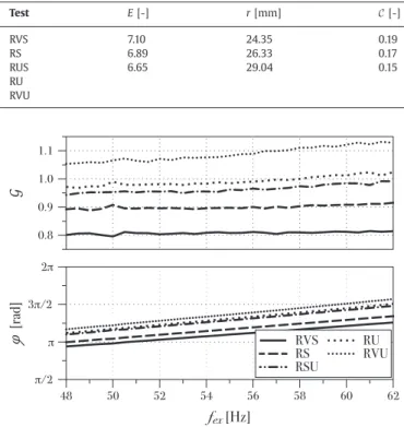
Figure
Documents relatifs
III High order velocity moment method for high Knudsen number flows 156 9 Eulerian Multi Velocity Moment (EMVM) model 158 9.1 Kinetic description of dilute gas-particle flows and
(27) are not fully accurate in this case; 2) the images, especially the ABI ones, have not been acquired at exactly the points of highest theoretical sensitivity (the curve of
Arch.. Le chapitre 2 s’attache à comprendre quelles sont les modalités d’intégration des familles nobles à la maison princière et les retombées dues à leur
Cette technique, qui permet notamment d’obtenir des lignées monoclonales, peut être employée sur toutes sortes de cultures, que ce soit pour l’isolation de
La première partie de ce document présente un état de l’art des travaux dans le domaine de l’extraction d’information à partir de données issues d’une
A statistical model for avalanche runout distance (Keylock et al., 1999) is used to obtain avalanche encounter probability as a function of avalanche size and location along the
Afin d’´ etudier l’efficacit´ e du mod` ele de poutre multifibre enrichi 2D d´ evelopp´ e dans ce travail de th` ese, ainsi que l’effet des ´ etriers sur le comportement non
En s’approchant, il découvrit son visage : il avait les yeux plutôt clairs mais qui ne jouissaient d’aucun charme, cernés de violet, ses pommettes
