Carpoolers classification while preserving users privacy

Carpoolers classification while preserving users privacy

Lucas Gülen

Master thesis for :

Master in Information Science - Data science

Supervisor :

Professor Douglas Teodoro

August 17th 2020

Disclaimer

This report is submitted as part of the final examination requirements of the Haute école de Gestion de Genève, for the Master’s of Science HES-SO in Information Science.

The use of any conclusions or recommendations made in or based upon this report, with no prej-udice to their value, engages the responsibility neither of the author, nor the author’s mentor, nor the jury members nor HEG or any of its employees.

The student has sent this document by email to the address given by his master’s thesis supervi-sor for analysis by the URKUND plagiarism detection software, according to the detailed procedure at the following URL: https://www.urkund.com .

"I certify that I have done this work alone, without having used sources other than those cited in the bibliography."

Done in Geneva, August 17, 2020 Lucas Gülen

Acknowledgments

First of all, I would like to thank my thesis supervisor, Dr. Douglas Teodoro, for his guidance, his advice and for all the ideas for exploration related to machine learning models and data throughout my thesis. Then, I would like to thank the company Mobilidée, more specifically Michalis Giannakopoulos Rochat, for having given me the opportunity to work on one of their business problems, for having welcomed me within their team and for having always been available to answer my questions related to the different problems that this thesis aimed to answer. I would also like to thank my friends and colleagues, Flavio Barreiro Lindo and Alex Perritaz, for supporting me, reading my thesis and advising me on some technical points related to machine learning. Moreover, I would especially thank Flavio Barreiro Lindo for the Portuguese cuisine that he made me taste and that allowed me to refocus on my work. Finally, I would like to thank my girlfriend, my friends and my family for their support and encouragement throughout this work and my studies.

Abstract

Carpooling is a mode of transportation that allows users to share places in their cars to reduce green-house gas emissions. Many services exist to encourage users to practice carpooling, while Mobilidée proposes a novel idea with a mobile application presented to other companies who want to promote soft mobility among their employees. Currently, Mobilidée already has an application that lets users enter manually whom they carpool with hand for how long. The advantage for any user is that the more they reports their carpooling data in the application, the more they will have a chance to receive incentives from his company. Thus, to ensure security in this process as much as possible, Mobilidée needs to automate data collection and analysis of their users’ smartphone sensors in order to deter-mine how much a given user has made carpooling in a given period. Indeed, today there is not a verification process in place that prohibits a user from claiming to carpool when, in reality, he does not. Hence, this work aims to investigate machine learning algorithms in order to classify people who made carpooling together or not automatically. This work will also explore some machine learning techniques to encode user data before their analysis to ensure their privacy.

Contents

Acknowledgments . . . iii

Abstract . . . iv

List of Tables . . . vi

List of Figures . . . viii

List of Equations . . . x Nomenclature . . . xii 1 Introduction 1 1.1 Context . . . 1 1.2 Objectives . . . 1 1.3 State-of-the-art . . . 2

2 Materials and methods 5 2.1 Data . . . 5

2.1.1 Descriptive analysis . . . 7

2.2 Data gathering tools . . . 13

2.3 Use cases . . . 17

2.4 Models . . . 18

2.4.1 General information . . . 18

2.4.2 Classification . . . 18

2.4.2.1 Linear regression to logistic regression . . . 18

2.4.2.2 Support vector machine . . . 23

2.4.2.3 Artificial neural networks (ANN) . . . 25

2.4.3 Regression . . . 40 2.4.3.1 Generative models . . . 40 2.5 Evaluation method . . . 44 2.5.1 Training . . . 46 2.5.2 Testing . . . 47 3 Results 49

3.1 Carpoolers classification - Original data . . . 49

3.1.1 Data preparation . . . 49

3.1.2 Model results . . . 51

3.2 Data encoding . . . 53

3.3 Carpoolers classification - Encoded data . . . 55

4 Discussion 58 4.1 Limitations . . . 60

5 Conclusion 61

List of Tables

2.1 Mobile sensor’s values example . . . 6

2.2 Passenger’s sample data matrix . . . 7

2.3 Dataset summary . . . 8

3.1 Linear models . . . 52

3.2 Neural network models . . . 52

3.3 Rnn-Lstm - Contingency table . . . 53

3.4 Autoencoder models . . . 54

List of Figures

1.1 GPS battery consumption - Magnetometer and accelerometer battery consumption . . . 4

2.1 Smartphone axes representation . . . 5

2.2 Travel distribution by class label . . . 8

2.3 Frames distribution by class . . . 9

2.4 Sensor’s autocorrelation coefficient . . . 10

2.5 Sensor’s sample normalised . . . 12

2.6 Sensors probability density distribution . . . 13

2.7 Ionic application - Login page . . . 14

2.8 Ionic application - Home page . . . 15

2.9 Ionic application - Use case page . . . 15

2.10 Ionic application - Invitation . . . 16

2.11 Ionic application - Passenger and driver ready view . . . 16

2.12 Ionic application - Travel running state (Passenger on left, driver on right) . . . 17

2.13 Convex vs non-convex function . . . 20

2.14 Linear regression line vs Logistic regression curve . . . 21

2.15 SVM - Linearly separable data - Decision surface . . . 23

2.16 SVM - Non-linearly separable data - Create new dimension . . . 24

2.17 SVM - Non-linearly separable data - Hyperplane decision . . . 24

2.18 Perceptron . . . 25

2.19 Multi-layer perceptron - MLP . . . 26

2.20 MLP - hidden unit k . . . 27

2.21 MLP - General weights unit update rule . . . 28

2.22 RNN-rolled . . . 29

2.23 RNN - Many-to-many - Computational graph . . . 30

2.24 RNN - Many-to-one - Computational graph . . . 31

2.25 LSTM - Many-to-many architecture . . . 33

2.26 LSTM - Forget gate . . . 34

2.27 LSTM - Input gate . . . 34

2.29 CNN - RGB image representation . . . 36

2.30 CNN - Convolution operation . . . 37

2.31 CNN - Non linearity function . . . 37

2.32 CNN - Max pooling . . . 38

2.33 Auto encoder . . . 40

2.34 Auto encoder - Layers disposition rule . . . 42

2.35 Gaussian distribution . . . 43

2.36 VAE Gaussian structure . . . 43

2.37 Confusion matrix - True labels vs Predictions . . . 45

2.38 McNemar - Contingency table example . . . 47

3.1 Data preparation - Frames . . . 50

3.2 Data preparation - Windows . . . 50

3.3 Data preparation - Windows merged matrix . . . 50

3.4 CNN data preparation . . . 51

3.5 Probability density distribution with 1 component (w_size = 5) . . . 54

3.6 Scatter plot of 2-components distributions (w_size = 5) . . . 55

3.7 Classifier based on encoded data . . . 56

3.8 Probability density plot with 1 component between latent space z and raw data . . . 57

List of Equations

2.2 Vector’s magnitude . . . 11

2.3 Vectors’ magnitude . . . 11

2.4 Linear regression generalised . . . 19

2.5 Mean squared error . . . 19

2.6 β optimisation - Normal equation - MSE . . . 20

2.7 Logistic regression - model formula . . . 21

2.8 Likelihood of observing data . . . 21

2.9 Maximum log-likelihood . . . 21

2.10 Conditional probability - logistic . . . 22

2.11 Maximum log-likelihood - Supervised learning - General formula . . . 22

2.12 Bernoulli distribution . . . 22

2.13 Likelihood function . . . 22

2.14 Maximum log-likelihood function - Supervised learning - Model formula . . . 22

2.15 Minimising negative log-likelihood . . . 23

2.16 SVM - new dimension . . . 24

2.17 SVM - Simple kernel - inner product . . . 25

2.18 Perceptron . . . 25

2.19 Perceptron loss function . . . 26

2.20 Perceptron loss function . . . 26

2.21 Derivative - chain rule . . . 27

2.22 Loss derivative with respect to wij- setp 1 . . . 28

2.23 Loss derivative with respect to wij- Terms simplification . . . 28

2.24 RNN - Operating formula . . . 30 2.24 RNN - Update equations . . . 32 2.26 LSTM - Forget gate . . . 34 2.27 LSTM - Input gate . . . 35 2.28 LSTM - Input gate . . . 35 2.29 CNN - Convolution 2D . . . 37

2.31 Auto encoder - Loss . . . 41

2.32 Bayes theorem - conditional probability . . . 44

2.33 VAE - Kullback-Leibler divergence . . . 44

2.34 VAE - Evidence Lower Bound (ELBO) . . . 44

2.35 Precision metric . . . 46

2.36 Recall metric . . . 46

2.37 F1 score . . . 46

2.38 McNemar Chi-square . . . 48

2.39 McNemar Chi-square example . . . 48

Nomenclature

Greek symbols

β Weights in linear regression β0 Bias in linear regression

δ Significance threshold µ Refers to mean

∇ Refers to the gradient of any function that follows ∂ Refers to partial derivative of any term that follows

σ Refers to the standard deviation or to the Sigmoid function in the machine learning context θ, ϕ Generally refers to any machine learning model or function parameters

Roman symbols

ˆ

y Model predictions

i Variable used as a row index j Variable used as a column index

L Refers to a general loss function used in machine learning n Variable used as the total number of values

P Refers to the probability of any term that follows

t Refers to a specific timestep in recurrent artificial neural networks W, V, U Matrix of weights, commonly used in machine learning models X Matrix of inputs, commonly used in machine learning models

x General notation for inputs data in machine learning models. Depending on the context, it could be also one of a smartphone sensor axis.

x0 Reconstructed output from an autoencoder or from a variational autoencoder

y True predictions in supervised machine learning models. Depending on the context, it could be also one of a smartphone sensor axis.

z Latent representation in autoencoder and variational autoencoder machine learning models. Depending on the context, it could be also one of a smartphone sensor axis.

1

Introduction

1.1

Context

The subject of this thesis is to investigate about assessing a carpooling classification problem without disclosing personal information. Carpooling is a mode of transportation that allows users to share places in their car in order to reduce greenhouse gas emissions [1]. Many services exist to encour-age users to practice carpooling, such as BlaBlaCar and Waze [2], [3]. A novel idea is proposed by Mobilidée with a mobile application [4] that is presented to other companies who want to promote soft mobility among their employees.

Currently, Mobilidée already has an application that lets users enter manually whom they carpool with and for how long. The advantage for any user is that more he reports its carpooling data in the application, more he will have a chance to receive incentives from his company. Thus, to ensure secu-rity in this process as much as possible, Mobilidée needs to automate data collection and analysis of their users’ smartphone sensors to determine how much a given user has made carpooling in a given period. On one hand, it will allow for fewer user interactions with the application and will decrease cheating probabilities. Indeed, today there is not a verification process in place that prohibits a user from claiming to carpool when, in reality, he does not.

1.2

Objectives

An important Mobilidée’s principle is to promote soft mobility among their employees, but among their proposed services too. So, a Mobilidée objective is to be able to encode user sensor’s data directly on the mobile before sending them to the server for further analysis.

Another significant Mobilidée’s principle is to protect as much as possible their customer’s data pri-vacy. In this respect, one of these thesis’ objectives is to be able to encode sufficiently user’s data collected to ensure the maximum privacy possible.

Moreover, the automated verification process mentioned in section 1.1 is not in place in Mobilidée. Thus, another objective in this thesis is to be able to use user data to determine whether a user made carpooling or not.

In addition, we do not have a data set at our disposal to reach the objectives cited above. Thus, as we aim to build some statistical models to achieve the two firsts objectives, we must find a way to gather a sufficient amount of data to obtain satisfying results. So this objective contains two

sub-objectives:

• Collecting and constructing a data set of lower-invasive mobile phone sensor data, • Use mobile sensors that consumes a small amount of battery power.

1.3

State-of-the-art

Data privacy

Data protection has become a central issue in the use of personal data processing systems due to the implementation of the General Data Protection Regulation (GDPR) in Europe since 2018 [5]. To address this issue, an approach has been adopted by Malekzadeh et al. They used a mobile autoen-coder to successfully encode sensor data from 24 users with a re-identification rate of 94% by their decoder and 7% of re-identification rate by a third party system which had no access to their trained decoder [6].

Malekzadeh et al. also published a scientific paper in which they used a replacement autoencoder and an anonymizing autoencoder to transform sensor data to preserve confidentiality and usefulness in disclosure. They managed to maintain a confidentiality loss of data of 7% and preserve their use-fulness of 92% [7].

To preserve the confidentiality of banking data, Maina et al. explored a type of algorithm called variational autoencoder (VAE). They managed to anonymize their data and maintain a Jaccard index ranging from 0.9 to 1 between the original data and the synthetics generated by the VAE [8]. The Jaccard index is a measure of similarity used by subtracting it from the number 1 to give the Jaccard distance. The closer this distance is to 1, the more substantial the similarity is.

Abay et al. also used a VAE in their research paper. Their goal was to use confidential data to generate synthetic ones following the same distribution, thus being usable in the same purpose and without any confidentiality constraint. With their model, they were able to generate synthetic data and obtained a lower classification error rate on these data than most of the current synthetic data generation got from another state-of-the-art algorithm [9].

To anonymize patient gait data, Ngoc-Dung et al. proposed an approach using a convolutional neural network. The network receives two gaits as input, the patient one to be anonymized, and another called "noise gait" and outputs the anonymized resulting data. Their method allowed them to achieve a failure rate in re-identification by third parties of 98.86% [10]. Another approach was used by

Ab-drashitov and Spivak, who used genetic clustering algorithms. In particular, they used L-diversity and k-anonymization to anonymize their data [11].

Time-series classification

One of the objectives of this research project is to be able to determine, based on mobile sensor data, whether two or more people are travelling in the same vehicle. Therefore, our approach will be to classify travelers using time series data from smartphone sensors. Thus, Kuk et al. have adopted an approach to classify time series data such as those from the mobile sensor data. They used mobile data from the accelerometer of many users travelling in a train, but in separate wagons, to assess the users were travelling together. Through using the Euclidian distance between users, they have achieved to have 93% of correct classifications [12].

In another approach, Nguyen et al. used magnetometer data from several London Underground users to classify people travelling together. They obtained a rate of correct classifications of 100% by using the Euclidean distance on the user magnetometer aligned data [13]. Lester et al. used accelerometer data from two smartphones to determine whether they were worn by the same person and in the same body location. Using the Fast Fourier Transform algorithm to convert the discrete accelerometer data into frequency data, they used a consistency function to measure the similarity of two frequency signals and achieved 100% accuracy over an average window of eight seconds of recorded data [14].

In order to recognize what activity a person was performing, based on the accelerometer, Zeng et al. used a convolution neural network. Their results were over 88% accurate [15].

Environmental concerns

In addition to being able to assess who has travelled together and how long they have travelled, this thesis aims to use sensors that use as least energy as possible and protect the privacy of people. As GPS is a sensor that consumes more energy than the accelerometer and reveals more confidential data about a user, such as their daily journeys, [16], it will only be used for comparison purposes in this work.

Moreover, according to Subhanjan et al., GPS would consume more smartphone battery than the magnetometer and the accelerometer combined. To reach this conclusion, they carried out tests on the use of GPS alone and the use of the magnetometer and accelerometer in another case, over 180 minutes [17]. Here is the graph they published in their scientific paper, where the "TrackMe" curve represents the use of the magnetometer and the accelerometer through their mobile application :

Figure 1.1: GPS battery consumption - Magnetometer and accelerometer battery consumption

Furthermore, according to Panichpapiboon et al., the accelerometer’s use as a substitute for the GPS sensor to estimate the average speed of a moving vehicle is possible and more accurate [18].

2

Materials and methods

2.1

Data

For this thesis, three mobile sensor’s data were chosen: the gyroscope, the accelerometer, and the magnetometer. Since they are motion sensors commonly used for user activity detection and user identification [14] [16] [13], they were chosen over other sensors such as the barometer, proximity sensor, and ambient light sensor. Each one has three axes, represented as x, y, z, and can be inter-preted as the three-dimensional space where the smartphone is located. Moreover, these three axes are in a fixed position relative to the smartphone, whatever the rotation or the force applied. Here is a graphical representation of the three-dimensional space used by all sensors in this thesis:

Figure 2.1: Smartphone axes representation

[19]

The accelerometer is one of the sensors which will be used. It measures how fast the acceleration changes, including physical acceleration and gravity, at a given time in m/s2_{[20] [21] in x, y and z axis}

and is given by the following formula:

distance

time = speed. (2.1)

There are two common types of accelerometers on the market: capacitance and Piezoelectric ac-celerometer. Usually, most of the commercialized smartphones use capacitive based techniques [22]. It works by sensing changes in capacitance between microstructures next to the accelerometer. Then it is translated into voltage for correct interpretation.

and the total magnitude of the magnetic field. Its units are micro Tesla and are written as µT . The magnetic forces applied on the mobile sensor’s magnetometer are due to the magnetic effect gener-ated by electric currents, magnetic materials near the sensor or Earth’s magnetic force [23].

Gyroscope is the third mobile sensor used in this work. It senses angular rotational velocity and acceleration [24]. All measures are reported in the x, y and z fields and values are expressed in radi-ans per second (rad/s) [20].

In this work, data from each sensor above is collected sequentially in different timestamps. It means that each data interval collected will have n frames of data where each frame has x, y and z values for each sensor. Thus, it could be interpreted as a time series where frame values are ordered by timestamp. Here is an example of mobile accelerometer’s data collected in 10 frames with a capture interval of 500ms:

Table 2.1: Mobile sensor’s values example Accelerometer Frame number x y z 1 0.04 4.32 9.75 2 6.91 0.55 4.18 3 1.92 -5.14 11.11 4 2.43 -1.65 9.05 5 2.73 -1.53 9.34 6 2.51 -1.70 9.31 7 2.55 -1.61 9.38 8 2.47 -1.71 9.20 9 2.44 -1.65 9.29 10 2.42 -1.56 9.39 n=10 interval=500ms

In Table 2.1, a minor variation can be observed in z axis which approximates the Earth’s standard acceleration gravity value of 9.807m/s2 _{[25]. One might assume that the z axis is facing the Earth’s}

core and so the smartphone screen too, according to Figure 2.1. This assumption could have been done on y axis if the smartphone was in a position where y was facing the Earth’s core.

The collected data are organized by travel with always a pair of one driver data matrix and one passenger data matrix. Each one has 12 features and is constructed like the sample of data shown in Table 2.2 below :

Table 2.2: Passenger’s sample data matrix

Accelerometer Gyroscope Magnetometer

x y z x y z x y z Magnitude Label 0.04 4.32 9.74 -0.19 -2.02 -0.60 1.50 2.81 -28.31 28.49 0 6.91 0.55 4.18 -2.19 0.50 0.22 -19.75 8.63 -17.81 27.96 0 1.92 -5.14 11.11 1.74 -1.26 -0.05 -22.25 7.69 -14.88 27.85 0 2.43 -1.65 9.05 1.74 -1.26 -0.05 19.88 6.19 -9.56 22.91 0 2.73 -1.53 9.34 1.74 -1.26 -0.05 4.00 12.81 -8.75 16.02 0 2.51 -1.70 9.31 1.74 -1.26 -0.05 -4.63 11.69 -9.75 15.91 0 2.55 -1.61 9.38 1.74 -1.26 -0.05 -7.44 8.50 -5.94 12.76 0 2.47 -1.71 9.20 1.74 -1.26 -0.05 -6.81 8.13 -5.38 11.89 0 2.44 -1.65 9.29 1.74 -1.26 -0.05 -5.94 7.94 -5.19 11.19 0 2.42 -1.56 9.39 1.74 -1.26 -0.05 -6.25 8.25 -5.56 11.75 0

All statistics and figures in section 2.1 will use the passenger file who is sampling in Table above. Each line of the Table 2.2 above represents a capture time (frame) for the passenger’s travel where each accelerometer, gyroscope, and magnetometer axes values are recorded. The last column is the label that could be "True" or "False" (1 or 0). When it is true, it means that the passenger and the driver of this trip were together at the current frame. Data used in Table 2.2 do not contain the timestamp field because of presentation concerns.

For each carpooling trip where there are more than two passengers, it is split into n − 1 trips, where nis the number of people in the car using the application. Every person is paired with the driver in order to simplify the data structure for the classification task. In fact, instead of mapping one driver with multiple passengers, it makes all combinations between the driver and the passengers to get n − 1trips of exactly one driver-passenger pair.

2.1.1

Descriptive analysis

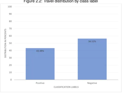
This section will discuss data distribution and try to make some preliminary assumptions. A critical thing to verify is that all classes are balanced as much as possible in our dataset. Thus, according to Batista et al. [26], some statistical models in machine learning tasks may compute much better results on a balanced dataset.

In this thesis, the classification task is a binary classification problem where a label can be either 1 (True / Positive) or 0 (False / Negative). The "Positive" value for a trip indicates that the passenger and the driver were together. Figure 2.2 below shows the proportion of each class over all trips in the data set. Therefore, there are 56.52% of negative instances where the driver and the passenger have generated data, but in two distinct vehicles. Hence, it could be assumed that the data set is balanced

in an acceptable manner where there is not a large gap between each class, given the 23 trips in total as seen in Table 2.3. The Table 2.3 also shows the minimum, maximum and the average of frames with respect to the entire dataset of trips.

Table 2.3: Dataset summary

Number of trips Min. frames Max. frames Avg. frames

23 3751 6508 5348

Figure 2.2: Travel distribution by class label

43.48% 56.52% 0 10 20 30 40 50 60 70 80 90 100 Positive Negative DISTRIB UTIO N IN PER CENTS CLASSIFICATION LABELS

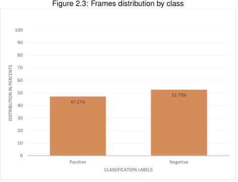
As shown in table 2.2, each travel has n frames. Each of these frames is associated with a label as well as the trip itself. As a trip may have variable number of frame depending on its duration, it could be interesting to know the classes’ distribution in terms of frames :

Figure 2.3: Frames distribution by class 47.27% 52.73% 0 10 20 30 40 50 60 70 80 90 100 Positive Negative DISTRIB UTIO N IN PER CENTS CLASSIFICATION LABELS

The Figure 2.3 shows similar results as Figure 2.2. However, it seems that class distribution is more balanced at a frames level, with 47.27% of positive frames and 52.73% of negative frames. Despite this little difference, we may consider that regardless of granularity level, the labels are balanced and allow us to work either with trips or frames directly.

To further understand the data, the autocorrelation coefficient can be used to analyze the relationship between the data. It is a metric that is often used in time-series analysis and measures how much a time-series is linearly related to the lagged version of itself [27]. It allows to know if a time-series is identically and independently distributed (iid) [28]. This is crucial information as in the machine learn-ing domain, the application of regression models implies a common hypothesis that assumes the data are iid [27]. Besides knowing the distribution, autocorrelation may help to find some seasonality and trends in time-series data [27]. The figure 2.4 shows the autocorrelation’s coefficient for each axis of each sensor with itself:

Figure 2.4: Sensor’s autocorrelation coefficient

The y-axis (vertical) units go from -0.5 to 1 and represent the autocorrelation’s coefficient. Despite y-axis plots on Figure 2.4 going from -0.5 to +1, the resulting output of autocorrelation’s coefficient can range from -1 to +1. The x-axis (horizontal) units represent the number of past values in the time-series and were arbitrarily chosen between 0 and 500. As an example, a positive autocorrelation value of 1 with a lag value of 5 noted i, assumes that if a i − 5 value in the time-series increased, the [i − 4, i] values would increase proportionally. On the other hand, a negative value of 1 with the same lag value assumes that a i − 5 value increase results in a proportionate decrease in the [i − 4, i] time-series values. An autocorrelation value of zero indicates no correlation between the i lag and the current time-series value.

In Figure 2.4, continuous gray lines represent a confidence interval of 99% and the dashed ones, represent a confidence interval of 95%. In this Figure, despite that the magnetometer’s

autocorrela-tion coefficient takes more lag steps to decrease, both the accelerometer’s and the magnetometer’s autocorrelation coefficient decrease as the lag steps increase and tend towards zero. At first glance, the gyroscope shows to be in the same case of magnetometer and accelerometer with a rapid de-crease in the autocorrelation coefficient. However, the data used to plot the Figure 2.4, sampled in Table 2.2, shows there are no real variations in all gyroscope axes over time. It is probably the reason why the autocorrelation value of the gyroscope is near zero. The general hypothesis given by Figure 2.4 is that the correlation of the time-series values of each sensor is insignificant from lag 50.

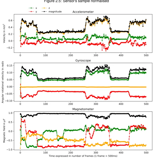
Figure 2.5 shows a normalized sample of the first 500 values for each sensor. The units depend on each sensor. Each plot has 4 curves representing x, y, and z axes and the magnitude between these axes. As a reminder, the vector magnitude also called the norm, where a is the time-series in our case, i is the index value and n is the last value of the time-series, is designed by Equation 2.2 [29]: ||a|| = q a2 1+ a22+ ... + a2n= v u u t n X i=1 a2 i. (2.2)

Thus, the plotted magnitude m in Figure 2.5 is calculated between x, y and z axes for each sensor and can be expressed by Equation 2.3:

||m|| = v u u t n X i=1 x2 i + n X i=1 y2 i + n X i=1 z2 i. (2.3)

The magnitude represents the norm of a vector and measures its length among all representations of this vector. In Figure 2.5, the black curve represents the distance between the three axes for each sensor and allows us to compare directly this magnitude between the sensors instead of comparing each axis independently. This figure shows the correlation between the magnitude of the accelerom-eter and the gyroscope. Both sensors have similar behavior, especially for the peaks and regularity of the magnitude.

Figure 2.5: Sensor’s sample normalised

Moreover, it would be relevant to know the distribution and how the data are spread. One way to do this is to compute each sensor’s time-series’ mean and standard deviation and compare them together. The other way, which would be visually more practical, is to plot the density, such as in Fig-ure 2.6. The Principle Component Analysis (PCA) has been used to plot each sensor with only one distribution curve instead of plotting the three-axis of each sensor. PCA may be used for dimension-ality reduction purposes, for example. In Figure 2.6, the vertical axis represents the probability of the horizontal axis values. Accelerometer and gyroscope have both a unimodal distribution, which results in a values interval being particularly dominant, among others. On the other hand, the magnetometer has a bimodal distribution. Another indication given by Figure 2.6 is that the distribution of accelerom-eter and magnetomaccelerom-eter are wider than the gyroscope. It could be explained by less rotational forces

applied on gyroscope than velocity forces applied on accelerometer and magnetic field applied on magnetometer in this trip.

Figure 2.6: Sensors probability density distribution

2.2

Data gathering tools

In this work, a data set that matches the classification problem has not been found. A way of col-lecting sensor’s data directly on a smartphone while people were carpooling had to be created. The chosen solution was to create a basic mobile application with Ionic v.5.4.16, a framework that allows developing hybrid mobile applications that can be used on both Android and iOS.

The server-side of the application uses Firebase as a database to store NoSQL data collected from the mobile sensors.

In the first data collection phase, the application has been used only by me and some friends, to be able to control the recording environment and to avoid collecting noisy data. In a second phase, which will be carried out after this work, the application will be distributed to Mobilidée’s employees to collect more data. The main functionalities of the application are :

• Create a trip, • Invite passenger(s),

• Start recording sensor’s data,

• Stop recording and send data to server.

Login

This had to be as simple as possible to let users type only their username to be connected. There is not any password, meaning a person takes the identity of another person. This is why the application needs to be used in a controlled environment, but there is no personal information stored in the application, other than the username. The main reason to create a login, in this case, is to list all potential passengers and be able to send them notifications. Here is the login page of the application:

Figure 2.7: Ionic application - Login page

The login page contains only one input field where the user must enter his username and a button, which allows him to connect. The available usernames are pre-configured in the Firebase administra-tive panel. Once a user has logged in, a notification token id is associated with the smartphone and is stored in Firebase backend.

Create trip

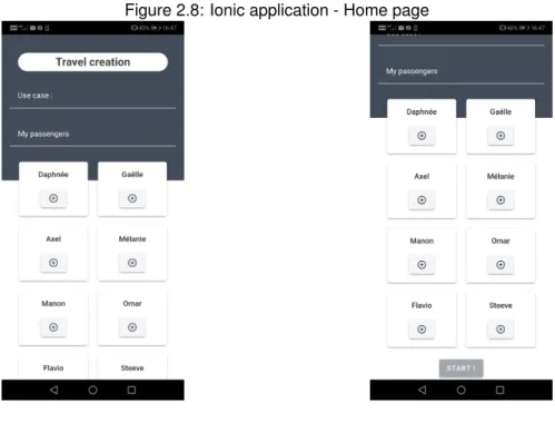
Once the user is logged in, there is a redirection to the home page. This page, illustrated in Figure 2.8, lets users create a trip by choosing the travel use case and by inviting passenger(s), which are explained and listed in the section 2.3. The only person on a trip who must fill in this page is the driver.

Figure 2.8: Ionic application - Home page

Inviting passenger(s)

Once the driver has chosen the correct use case for the trip in the page showed in Figure 2.9:

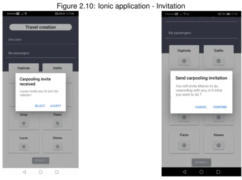
The driver must invite one or multiple people listed on the home page to join his trip in order to be able to begin recording the sensor’s data. When the driver selects a passenger, a popup will be displayed to ask his confirmation, and once it is done, the notification goes directly on the smartphone of the selected passenger. The left side of Figure 2.10 is the passenger’s view, and the right side is the driver’s view.

Figure 2.10: Ionic application - Invitation

Once the passenger has accepted the invitation, he will be redirected to the view showed on the left side of the Figure 2.11 and the driver’s view will be updated as the right side of the same figure.

Start recording sensor’s data

The travel is now ready to start with one driver and one passenger. Both driver and passenger must tap on the "Start" button to begin mobile’s sensors recording. The first time the users start a carpooling trip on the application, a confirmation will be asked to collect sensors data, according to the GDPR. During the trip, sensors data will be recorded every 500 milliseconds. This was an arbitrary choice to try to capture as many variations as possible in the magnetometer, accelerometer, and gyroscope without consuming too much battery. Too small of an interval could cause the battery to run low. The application’s state while travel is running is shown in Figure 2.12.

Figure 2.12: Ionic application - Travel running state (Passenger on left, driver on right)

Stop recording data

Finally, both driver and passenger has to press the button "Stop" illustrated in Figure 2.12 to conclude the carpooling trip. It will send their raw data to the firestore, a local version of firebase that allows data to be temporarily stored on the mobile if it has no internet connection; otherwise, it sends them directly to the database. The application’s state is reset to its initial state, as shown in Figure 2.8.

2.3

Use cases

The use cases treated in this section refer to possible scenarios that could happen in a carpooling trip. These scenarios have been discussed with Mobilidée and the thesis supervisor to cover a large scope of cases that could happen in reality. As shown in section 2.1, the mobile sensor’s axes are fixed, so it has been decided to use different smartphone positions and variate people’s activity during the carpooling travel. The use cases, briefly shown in Figure 2.9, are the following:

2. Driver and passengers travel in same vehicle, driver’s smartphone in his pocket, passenger’s smartphone in movement (playing a game i.e).

3. Driver and passengers travel in same vehicle, driver’s smartphone fixed, passenger’s smart-phone in pocket.

4. Driver and passengers travel in different vehicles with different trajectories, smartphones at rest. 5. Driver and passengers travel in different vehicles, but one following each other, smartphones at

rest.

6. Driver start travel alone, passengers getting in the car only near destination, smartphone at rest. Only the use case number 1 and 4 cited above would be considered for the data collection made in this thesis. Furthermore, I am the only one who collects the data with multiple smartphones. These decisions were made to be able to keep data collection under control while minimizing the risk of noisy data wrongly recorded by users, for example. A first data collection was made, introduced in section 2.1, to be able to train statistical models. A second data collection in a more real environment would be done after this thesis to test the trained models. In this second phase, most of the use cases cited above would be considered, and the data collection application would be distributed to most Mobilidée employees. The second phase will not be discussed in this thesis.

2.4

Models

2.4.1

General information

This section will discuss the different statistical models used in the classification and regression prob-lems, as the scope of this thesis will approach both. Machine learning models might be represented as a set of weights applied on a dataset to give a prediction. Depending on the task to solve, predic-tion can be discrete and denoted as classificapredic-tion, or they can be continuous and would be denoted as regression. Then, the model’s objective is to train on a data set to minimize a loss function (rep-resents the error of the model), noted L, by changing these weights, noted W . In statistics, the loss function is used for parameter optimization such as W , and consists of a difference between expected output and model’s output.

2.4.2

Classification

2.4.2.1 Linear regression to logistic regression

As a reminder of section 1.1, the classification model architectures discussed here are related to carpooling classification. One of the most simple statistical models used in machine learning is the

linear regression algorithm. This model makes a linear relationship assumption between a scalar prediction, noted y, and one or more explanatory variables, noted x. Thus, linear regression uses as many parameters, noted β, as explanatory variables, also called features, and chooses those who minimize the prediction error. Equation 2.4a illustrates the linear regression model applied on each dataset instance where yi is the prediction for the ith instance, β0 is the bias, n is the number of

features and so the xij is the jth feature for the ithinstance. Moreover, the linear regression might

be written as the matrix approach, as shown in equation 2.4b, where W is the β matrix, or more generally, the weights matrix and X is the features matrix.

yi= n X j=1 βj· xij+ β0, (2.4a) y = WTX. (2.4b)

Once the model has obtained the predictions y, its’ objective will be to choose the best W to minimize the loss function. Mean squared error (MSE) is a used loss function in linear regression and is expressed as follow: M SE = 1 n n X i=1 (yi− ˆyi)2. (2.5)

MSE will calculate the squared average difference between the model output ˆyand the correct label y expected, which must be minimized to obtain the most accurate model. Two approaches could compute this minimization:

• Analytical solution, • Gradient descent.

The analytical solution exists because the MSE in linear regression is a convex function, which means there is only one minimum, see the left side of Figure 2.13. This minimum might be found by using the partial derivatives of MSE with respect to w and with solving the equation by finding the only one existing 0.

Figure 2.13: Convex vs non-convex function

[30]

As the matrix analytical solution showed in Equation 2.6 requires a matrix inversion calculation which his cost growth as the number of features increase, gradient descent is commonly preferred.

β = (XTX)−1XTY. (2.6)

The gradient descent part is a fundamental concept to keep in mind as it will be used in many ma-chine learning loss minimization problems. It is an optimization algorithm that iteratively moves in the steepest direction of a function by taking its’ negative gradient. The gradient is a term to designate a vector in which every position is a partial derivative of a multi-variate function. Hence, as the deriva-tive of a function gives the direction of the highest increase, taking the negaderiva-tive gradient will follow the fastest direction that minimizes the function output.

The usage of linear regression is limited, especially in binary classification, such as in carpooling classification discussed in this thesis. Indeed, the outputs produced by the linear regression could be any real number. This approach does not allow for probabilistic analysis. However, negative values could represent one class and positive values in another class. The problem with this technique is for optimizing the statistical model since the outputs are not normalized between 0 and 1, for example. Figure 2.14 shows another algorithm that can address this issue, the logistic regression while showing the difference between linear regression and logistic regression [31].

Figure 2.14: Linear regression line vs Logistic regression curve

[31]

The solution is to use a logistic function, such as sigmoid, on linear regression model predictions to obtain probabilities between 0 and 1. See the logistic application on linear regression output data on right side of Figure 2.14. This model is called logistic regression, and its predictions could be obtained by the Equation 2.7 where σ is the logistic function.

y = σ(WTX + b). (2.7)

Instead of minimizing the MSE as in linear regression, the logistic regression parameters optimization will choose the parameters to maximize the probability. This is known as the maximum likelihood estimation (MLE). The MLE’s general intuition is to maximize the conditional probability of observing the data given probability distribution of X and its parameters θ:

maxL(X|θ). (2.8)

As X is the joint probability distribution of all observations, Equation 2.8 could be written as the sum of the conditional probability, as shown in Equation 2.9. Moreover, the logarithm function is com-monly used to avoid unstable numerical issues caused by multiplying multiple probabilities together. Furthermore, using the logarithm function on another function will not change its’ argmax.

max

n

X

i=1

log(P (xi|θ)). (2.9)

In the literature, it is commonly known as the log-likelihood function. In supervised learning, by following the underlying logic of Equation 2.8, the problem could be expressed as the conditional

probability of an output y given the inputs X:

P (y|X). (2.10)

Thus the definition of maximum likelihood in supervised learning can be rewritten as follow:

max

n

X

i=1

log(P (yi|xi; Q)). (2.11)

where Q is the logistic regression model. To use maximum likelihood function, a probability distribution needs to be assumed. The binomial probability distribution is the most often used in classification problem with two classes [32], which is defined by the following formula:

p · k + (1 − p)(1 − k) f or k ∈ {0, 1}. (2.12)

where p is the probability, and k is the possible outcomes. Hence, this probability distribution can be extended to the logistic regression model where the probability σ(WT_{X)is the output of the model,}

and the possible outcome y is the correct label given by the data set, as illustrated in Equation 2.13.

L = σ(WTX) ∗ y + (1 − σ(WTX)) ∗ (1 − y). (2.13)

The likelihood function needs to be maximized and computed for all instances in the data set, where nis the number of instances. Please, see the equation 2.14, which also uses the logarithm function to avoid numerical issues, as discussed previously in this section.

L = argmax1 n n X i=1 log(σ(WTxi)) ∗ yi+ log(1 − σ(WTxi)) ∗ (1 − yi). (2.14)

Besides, it is common to minimize the loss function in machine learning optimization problems rather than maximize it. Hence, the negative of the likelihood function minimization instead of the log-likelihood maximization function is used, as shown in Equation 2.15

L = argmin1 n n X i=1 −(log(σ(WT_x i)) ∗ yi+ log(1 − σ(WTxi)) ∗ (1 − yi)). (2.15)

The Equation 2.15 is in fact the binary cross-entropy loss. As the MSE discussed above in the linear regression, cross-entropy is used to compute an average error between the predicted label and the true label. As the cross-entropy is not a convex function, an iterative optimizing algorithm, such as the gradient descent explained above, must be used to find the best logistic regression weights W .

2.4.2.2 Support vector machine

Support vector machine (SVM) is a supervised machine learning algorithm initially designed for two-group classification problems[33]. SVM aims to create a decision boundary, also called hyperplane, based on sample data that allows separating classes in space to classify other instances of data efficiently. Two groups of SVM can be found: the one who is used on linearly separable data and the one on non-linearly separable data. In the linear case, the SVM tries to find the hyperplane that separates each class while maximizing the hyperplane and support vector’s margin. Support vectors are found by using the closest point of each class to the hyperplane, and the margin is the distance between the hyperplane and the support vectors, see Figure 2.15 where each color and shape corresponds to a different class.

Figure 2.15: SVM - Linearly separable data - Decision surface

[34]

In non-linearly separable data, a straight line, as in Figure 2.15, cannot separate the data into two distinct classes. Considering the left side of the Figure 2.16 where data from two classes are shown in two different colors, SVM will create a third dimension to try to make a clear separation between classes as shown in the right side of the Figure 2.16.

Figure 2.16: SVM - Non-linearly separable data - Create new dimension

Then, SVM will create a hyperplane to separate the data into classes in the three-dimensional rep-resentation shown in the left side of Figure 2.17 and could be seen in two dimensions by converting the data back to its original representation and see how the hyperplane looks like in the right side of the Figure 2.17. The third dimension z here is computed the Equation 2.16 where x and y are two features of the data set.

z = x2+ y2 (2.16)

Figure 2.17: SVM - Non-linearly separable data - Hyperplane decision

SVM’s technique when dealing with non-linearly separable data is to find the best function to map data from one space to another space, which is more straightforward for SVM to manage. It is common to use kernel functions, such as Radial basis function (RBF), polynomial kernels, and Gaussian kernels, to reduce the complexity of finding the mapping function. Assuming the data to analyze are vectors, a simple kernel example that respects kernels’ fundamental property would be the inner product of two vectors [35]. See the Equation 2.17 where x and y are two dataset feature vectors and n is the number of instances.

k(x, y) = xTy =

n

X

i=1

xiyi. (2.17)

This kernel function is usually called the linear kernel. Much more complex kernel methods, as cited above, are often used in SVM; however, we will not discuss them in more detail in this thesis.

2.4.2.3 Artificial neural networks (ANN)

Perceptron

The Perceptron, developed in 1958 by F. Rosenblat, is the simplest example of neural network ar-chitecture and was designed with the main idea of having some of the fundamental properties of the human brain system [36]. Indeed, the Perceptron architecture contains only one neuron layer with one single neuron, as shown in Figure 2.18, where a are the predictions, the "Sum" and the "Activation function" units are parts of the Perceptron neuron.

Figure 2.18: Perceptron

[37]

The Equation 2.18 gives the mathematical way to get a prediction for the kth_{instance from a}

Percep-tron where n is the number of instances in the training data, b is the bias that controls the y-intercept, and σ is a non-linear activation function such as ReLu, Sigmoid or Tahn.

yk = σ( n

X

i=1

Assuming the activation function is a Sigmoid in above Equation, the Perceptron will make similar pre-dictions as logistic regression, see Equation 2.7. The difference lies in the Perceptron not assuming a Bernoulli distribution and is more flexible with the possible activation functions, such as ReLU instead of Sigmoid. Moreover, the Perceptron only penalizes instances that are wrongly classified. Thus, the Perceptron loss function is defined by equation 2.19, where M is the set of misclassified instances.

− X

xi∈M

(wTxi+ b)yi. (2.19)

Then, the Perceptron’s loss function minimization needs to be computed with the gradient descent to find the optimal weights. The gradient of the loss function is then defined by Equation 2.20.

∇L(w) = − X

xi∈M

xiyi. (2.20)

Multi-layer perceptron (MLP)

The Perceptron can only solve linear problems while the multi-layer perceptron has not this limitation, which is a type of feedforward artificial neural network. The term feedforward designs the fact that the connections between the nodes, inside the network, do not form a cycle. MLP architecture consists of having an input layer, an output layer, and at least one hidden layer. The hidden layer is composed of multiple perceptron units; see Figure 2.19. MLP is a fully-connected network where each node in a specific layer is connected with a certain weight wijto every node in the following layer.

Figure 2.19: Multi-layer perceptron - MLP

[38]

maps the hidden layer results to the desired output. In a multiple label classification problem, the softmax activation function could be used as the output non-linear function to map the hidden layer results to a probability to belong in each class. The main difference between sigmoid and softmax non-linear function lies in the output properties. Either Sigmoid and Softmax outputs lie between 0 and 1; however, the sum of the softmax outputs always gives 1 and can be interpreted as probabilities.

Any perceptron unit in any hidden layer will always have the same operation: receiving input ak from

the previous layer which is given by the weighted combination of the outputs of the previous layer and weights wk of the current layer where current unit k applies a non-linear activation function f . See

Figure 2.20 where a hidden unit k receives activation value ak, the output from the previous layer z

and use the weights wk of the current unit k.

Figure 2.20: MLP - hidden unit k

Similar to the hidden layers, each k output unit gets as activation the linear combination of the previous layer output with the output weights. Hence, each k unit in an MLP has a set of j weights representing a weights matrix of j · k parameters to optimize. For example, assuming a dataset of instances with 200 features each using an MLP with one hidden layer of 50 units, there will be 50 × 200 = 10000 parameters to train only for the hidden layer. To be able to learn all these parameters, the backpropagation of the error with respect to the weights w must be computed. This notion refers to the partial derivative of the loss function with respect to any weights in the MLP. The intuition behind this calculation tells how quickly the error changes when the weights change[39]. Before going further, an essential notion is the chain rule; see Equation 2.21. It is used when the derivative of a composite function needs to be computed [40].

(f (g(x)))0 = f0(g(x)) · g0(x) ≡ ∂dz ∂dx = ∂dz ∂dy · ∂dy ∂dx. (2.21)

a composition of multiple functions. Thus, to backpropagate the error through the weights of the MLP, the partial derivatives using the chain rule will be used. Let’s assume a loss function L(w), which is usually the cross-entropy in a binary classification problem, computed on the MLP outputs shown in Figure 2.19, which has to be minimized with respect to the weights w. By doing only the first partial derivative step from the output to the hidden layer, assuming w contains only weights from j to i unit links between the output layer and the hidden layer. The contribution of a wij weight to the L comes

only through the activation level aiwhich is given by Equation 2.22:

∂L ∂wij = ∂L ∂ai · ∂ai ∂wij . (2.22)

Equation 2.22 gives the gradient of the error with respect to wij which connects the output of unit j to

the input of unit i where a terminology simplification can be done as:

∂L ∂ai = δi, (2.23a) ∂ai ∂wij = zj, (2.23b) ∂L ∂wij = δizj. (2.23c)

Thus, this gradient is used as the weight update rule for each hidden layer in any MLP as it may contain multiple hidden layer. More generally, the weights update rule inside a unit may be expressed as ∂L_∂z · ∂z

∂w for one hidden layer, as shown in Figure 2.21.

Figure 2.21: MLP - General weights unit update rule

with respect to its input. The local gradients refer to the gradient of the current node output with re-spect to the current input. The downstream gradients refer to applying the chain rule by multiplying the upstream gradient with the local gradients and passing them through the previous node in the network to continue backpropagation of the error.

In Figure 2.21, two downstream gradients are computed : one with respect to the weight parame-ter w and another with respect to the input x. Assuming that x is the input given to the network, the error gradient with respect to it does not need to be calculated. However, assuming that x is given by another hidden unit, its gradient must be computed to continue passing backward the propagation of the error since the input layer where only the gradient with respect to w has to be done.

Reccurent neural networks (RNN)

RNN is a type of artificial neural network where previous outputs are used to predict further outputs. The RNN assumption is that a single input item in a given series is related to others as it uses the information of previous input to help him taking predictions on further ones. In other words, the RNN decision on an instance is influenced by what it has learned from its past features, in addition to the other instances’ influence on the network in general. A known advantage of RNN among feedforward neural networks is that they are designed to allow dynamic vector sizes as input. An important notion here is the timestep, a common term used in RNN about specific variable states at a given time in the network, noted t. Furthermore, the RNN architecture has a single hidden layer, which takes as input the data xt _{and the previous output made on data to give an output at}

the current timestep, see Figure 2.22. Colah’s quote may exemplify an analogy between how RNN works and how Human understands the natural language: "You understand each word based on your understanding of previous words. You don’t throw everything away and start thinking from scratch again. Your thoughts have persistence" [41].

Figure 2.22: RNN-rolled

The RNN illustrated in Figure 2.22 shows two ways of representing how it works. On the left side, it shows the RNN, commonly known as the rolled representation, at a given timestep t where the hidden layer A taking some input xtand outputs a value htwhere the arrow recursively pointing on A

represents the information passed to the t + 1 timestep. On the right side of the Figure 2.22, it shows the RNN, commonly known as the unrolled representation, at some multiple timestep from 0 to t. The information passed through the timesteps is more obvious in this representation where each xtinput

gives an output htand let information to the next timestep t + 1. This can be formulate by Equation

2.24 where h(t)_{is a function f of h}(t−1) _{and x}(t)_{where θ are the parameters of f .}

h(t)= f (h(t−1), x(t), θ). (2.24)

The RNN can also be expressed with a computational graph that maps an input sequence x to a cor-responding sequence of output o, commonly called many-to-many, see Figure 2.23. A computational graph is a directed graph where each node refers to operations or variables.

Figure 2.23: RNN - Many-to-many - Computational graph

[42]

In Figure 2.23, the loss function L measures the difference between the model prediction o and the target value y. A weights matrix of U parametrizes connections between x and the hidden layer while the hidden layer is parametrized with a weights matrix of W by itself through timesteps of t, and the

hidden layer to the output layer is parametrized with a weights matrix of V .

One may use this architecture to generate text. At training time, it will work like a feature extractor by trying to predict the next word in a given sentence where each component of x would be a word given to the RNN that would try to find the next word of yt by predicting otat a given timestep of t. This

architecture uses a little trick, such as when testing time, the model generates a sentence, word after word, by passing through the previous word predicted to help it generate the next one and output the final tense without any input.

This leads to another architecture used in this thesis, where the RNN maps an input sequence of x to only one output of o. This is commonly referred as many-to-one RNN architecture and can also be shown as a computational graph, see Figure 2.24 which uses the same notation as Figure 2.23 except τ which represents the last step in the x input sequence.

Figure 2.24: RNN - Many-to-one - Computational graph

[42]

Hence, the Equations 2.25a, 2.25b, 2.25c, 2.25d mathematically expressed the operations computed to get a prediction for any timestep from t = 1 to t = τ , where c and b are bias vectors, and tanh is a

non-linearity function. a(t)= b + W h(t−1)+ U x(t), (2.25a) h(t)= tanh(a(t)), (2.25b) o(t)= c + V h(t), (2.25c) ˆ y(t)= sof tmax(o(t)). (2.25d)

Furthermore, the Equations 2.25a and 2.25b are used at every timestep, in the many-to-one case, to be able to accumulate information until the end of the input sequence where the Equation 2.25c and 2.25d will be used. To compute this model’s error with respect to its parameters W, V, U, b and c, a loss function must be used. Let’s assume a loss function L, which has to be minimized with respect to each of the parameters mentioned. The gradient of the loss respect each of these has to be computed with backpropagation through time, and weights optimization will be found by using gradient descent. The backpropagation through time refers to the gradient that is computed through each timestep.

Long short-term memory (LSTM)

The long short-term memory architecture is a kind of RNN capable of learning long-term dependen-cies which its objective is to try to solve the vanishing and exploding gradient problem encounter with basic RNN. The vanishing gradient problem occurs when the gradient value of the loss with respect to a parameter becomes extremely small and does not contribute any more to the parameter update. The exploding gradient occurs when gradient value increases so much that the parameter update tends towards infinity. As in basic RNN, the gradient is computed through time, the probability of hav-ing vanishhav-ing and explodhav-ing gradient is increased by the number of timesteps to go through. Thus, having a basic RNN with long sequences as input may increase the probability for the model to forget what it learned at the beginning of a sequence and only allow it to have a short memory.

The LSTM works such as a basic RNN where it treats input data as sequence and also has a hidden layer A which receives a hidden state h, a cell state c and a component of the input sequence x at each timestep t, see Figure 2.25.

Figure 2.25: LSTM - Many-to-many architecture

[41]

One of the differences with a basic RNN lies in the internal treatment of the hidden layer. Indeed, multiple sigmoid activation functions are applied to regulate the information that is passed through timesteps in the network and is commonly called gates. Here are the three sigmoid gates, also noted σin Figure 2.25 :

• Forget gate, • Input gate, • Output gate.

When a component of x input sequence is given to the hidden layer of the LSTM, the forget gate is the first operation computed, see Figure 2.26 where ht−1is the hidden state at the previous timestep,

xtis the current component of x and ftis defined by Equation 2.26 where Wf is a weight matrix and

Figure 2.26: LSTM - Forget gate

[41]

ft= σ(Wf· [ht−1, xt] + bf). (2.26)

As a sigmoid function is applied on the previous information ht−1and the current input component xt

which gives a value between 0 and 1, the role of the forget gate is to decide what information to throw away from the cell state ct−1by a multiplication operation. Then, it is the turn of the input gate, see

Figure 2.27 where ˜Ctis the new cell state and it, a vector used for scaling. ˜Ctand itare respectively

defined by Equations 2.27a and 2.27b where Wi, Wcare weight matrix and bi, bcare bias vectors.

Figure 2.27: LSTM - Input gate

[41]

˜

it= σ(Wi· [ht−1, xt] + bi). (2.27b)

The role of the input gate is to decide what information to add to the cell state Ct−1˜ where it is a

vector result of sigmoid application with values between 0 and 1 that will scale the update ˜Ct by

a multiplication operation, see the left side of Figure 2.27. It will then add information, with a vector addition operation, to the cell state Ct−1that will be the final output cell state Ctof the current timestep.

It is finally the turn of the output gate; see Figure 2.28 where ht is the hidden state of the current

timestep that is transmitted to the future timestep.

Figure 2.28: LSTM - Output gate

[41]

ot= σ(Wo· [ht−1, xt] + bo), (2.28a)

ht= ot· tanh(Ct). (2.28b)

The role of the output gate is to decide what information to output to the future timestep. Through its sigmoid value between 0 and 1, the otcomponent will scale the information to output by multiplication

with Ct. A crucial property in LSTM is that the cell state only regulates the information to keep or

remove in the hidden state, which is the information that navigates through timesteps and helps the model keep in memory the past input component information from x.

Convolutional neural network (CNN)

CNN is a feed-forward artificial neural network architecture that was biologically inspired on the work-ing of the neurons of the visual cortex [43]. Hence, it has been used in many image classification

task [44], [45], but also in text classification [46], [47] and time series classification problem [48]– [50]. A typical CNN layer consists of three stages with the last layer that allows the network to make predictions [51]:

1. Convolution. 2. Non linearity. 3. Pooling.

4. Classification / Regression.

In order to discuss the fundamental operations of a CNN mentioned above, all the explanations will take an image classification task as an example. Moreover, an image can be considered a three-dimensional matrix, such that each dimension is an integer matrix, or channel, containing values between 0 and 255. Each of these dimensions refers to the separated Red, Green, and Blue (RGB) colors of the picture where each index contains the corresponding pixel color value, see Figure 2.29.

Figure 2.29: CNN - RGB image representation

[52]

The convolution layer aims to extract features from the input image while preserving the image pixels’ spatial relationship. It is a method where an integer matrix, commonly called kernel or filter, is passed over an image and transform it based on filter values which can be mathematically formulated as an element-wise multiplication between a weight matrix W and sub-parts of the image x, see Figure 2.30 where x is an input of nH· nW size, filter size f = 3 · 3, stride s = 1 and padding p = 0. The stride

indicates the filter step on the image. It is essential to remember that filters act as a feature detector in the original input picture and give a result that can be called a feature map.

Figure 2.30: CNN - Convolution operation

[53]

According to the Equation 2.29, the feature map F of size m · n is calculated such as the input image is denoted by x and the kernel filter by f . F rows and columns indexes are marked with m and n while the kernel filter matrix f rows and columns are noted as j and k, respectively.

F [m, n] = (x · f )[m, n] =X

j

X

k

f [j, k]x[m − j, n − k]. (2.29)

The next step is to introduce non-linearity in the network by applying an activation function, such as ReLU, on the convolution layer results. ReLU will be applied per pixel as an element-wise operation and will replace all negative values with zero; see Figure 2.31 where ReLU function R(z) will take the maximum value between 0 and a given input z.

Figure 2.31: CNN - Non linearity function

Then, the spatial pooling has to be done in order to reduce the dimensionality of the feature map while keeping important information. The pooling can use different mathematical functions such as the maximum, the average, or the sum. In any case, the pooling operation helps to make the repre-sentation invariant to small translations of the input. Invariance to translation implies that if the input is translated by a small amount, the values of the pooled outputs do not change [51]. Assuming the max-pooling was chosen, a pooling size has to be set and by sliding the pooling window on the image, the maximum value in each region of the pooling window has to be taken, see Figure 2.32 where the stride s = 2 and the pooling window size is 2 · 2.

Figure 2.32: CNN - Max pooling

[55]

The three blocks discussed above (convolution, non-linearity, pooling) could be repeated to expand the network before having the last layer, which will be a fully connected one. This refers to a layer that flattens the last pooling layer into one dimension and maps it with an output layer. Indeed, the fully connected layer is an MLP with a final output layer that allows the model to make predictions. Such as the three layers that can be stacked multiple times to have a deeper network, it is common to use multiple fully connected layers with a progressive size reduction in the number of units before having the final output layer.

In addition to their ability to capture features in images, the CNN architecture also allows a com-putational cost reduction as each pooling layer reduces the size of the image initially given in input and, thus, reduces the total number of parameters to optimize in the network, compared to traditional artificial neural networks. In the different principal components example of CNN above, a convolution in two dimensions was used. However, one dimension convolution is also commonly used. Instead

of using the input data as a two-dimensional matrix, the one-dimensional convolution uses input as a vector. The operation is the same as two-dimensional convolution and is commonly used with time series data as they are usually represented in one dimension.

2.4.3

Regression

This section will discuss different model architectures used in this thesis for user privacy preservation. In order to use users mobile sensors data while not divulging personal data, some models would be considered in this section, such as generative models. This section’s regression term refers to all its related models that will no try to solve a classification problem. Indeed, the models will try to map each input x with itself as x is composed of continuous time-series values that constitute, by definition, to a regression problem.

2.4.3.1 Generative models

Generative models are a branch of unsupervised learning, where unsupervised learning relates to models that work to discover patterns in the data and not predict a given label. Generative models can generate new samples that follow the same probabilistic distribution of a given dataset [56] by estimating the probability density function.

Auto encoder (AE)

The auto encoder (AE) is a type of artificial neural network that attempt to copy its inputs as outputs [42].The internal operation of the network may be viewed with two distinct parts, as illustrated in Figure 2.34 : the encoder function f (x) which might be expressed as Equation 2.30a and the decoder function that try to produce a data reconstruction x0and formulated as Equation 2.30b.

Figure 2.33: Auto encoder

h = f (x), (2.30a)

x0 = g(h). (2.30b)

The AE objective is to reproduce the inputs as outputs. Thus, one may assume that the utility of such an architecture is that h, also called latent space or z, should ideally learn useful properties from x before reconstructing it as x0_{. Hence, the learning of useful properties might be more relevant}

than the decoder inputs reconstruction task itself. In order to obtain the most salient features of x, a standard method consists of constraining h of having fewer dimensions than x, and this architecture type is called an under complete AE [42]. The under complete AE with a linear decoder is commonly compared to the principal component analysis (PCA) as both learn a subspace of x and compute a dimensionality reduction as side-effect [58]. Moreover, h could have as many dimensions as x, and in the overcomplete case, it could have higher dimensions than x. In both cases, the decoder can learn to copy the inputs as outputs without necessarily learn useful h data distribution.

The loss function used in AE is usually the mean squared error where the objective is to minimize the dissimilarity of x0 _{with x, see Equation 2.31 where θ is the parameter of f , ϕ is the parameter of g,}

and n is the number of instances in the data set.

L(θ, ϕ) = 1 n n X i=1 (xi− fθ(gϕ(xi)))2. (2.31)

Concerning the AE architecture, both encoder and decoder could use any neural network architecture such as those described in section 2.4.2.3. However, the decoder must have the same number of layers as the reverse order’s encoder part. That means, assuming an encoder with 3 layers going from an input size of 10 to an output size of 6, the decoder should have the same layers. However, the decoder inputs size will go from 6 to 10, in order to reduce dimensions first in the encoder and increase them in the decoder to recover the same shape as original inputs, see Figure 2.34.