HAL Id: hal-01471566
https://hal.uca.fr/hal-01471566
Submitted on 20 Feb 2017
HAL is a multi-disciplinary open access
archive for the deposit and dissemination of
sci-entific research documents, whether they are
pub-lished or not. The documents may come from
teaching and research institutions in France or
abroad, or from public or private research centers.
L’archive ouverte pluridisciplinaire HAL, est
destinée au dépôt et à la diffusion de documents
scientifiques de niveau recherche, publiés ou non,
émanant des établissements d’enseignement et de
recherche français ou étrangers, des laboratoires
publics ou privés.
Fast loop-free transition of routing protocols
Nina Bekono, Nancy Rachkidy, Alexandre Guitton
To cite this version:
Nina Bekono, Nancy Rachkidy, Alexandre Guitton. Fast loop-free transition of routing protocols.
84th Vehicular Technology Conference (VTC), IEEE, Sep 2016, Montreal, Canada. �hal-01471566�
Fast loop-free transition of routing protocols
Nina Pelagie Bekono, Nancy El Rachkidy, Alexandre Guitton
Clermont Universit´e, Universit´e Blaise Pascal, LIMOS, BP 10448, F-63000 Clermont-Ferrand, France CNRS, UMR 6158, LIMOS, F-63173 Aubi`ere, France
Emails:{nina pelagie.bekono, nancy.el rachkidy, alexandre.guitton}@univ-bpclermont.fr
Abstract—In networks that operate during a long time, the routing protocol might have to be changed (in order to apply a routing protocol update, or to take into account a change in the routing metrics). A loop-free transition algorithm has to be used in order to perform the transition to the new routing protocol without generating transient routing loops. In this paper, we propose a loop-free transition algorithm called ACH (avoiding cycles heuristic), which is able to perform the transition in a very small number of steps. Compared to other algorithms of the literature, ACH yields a number of steps which is independent of both the number of nodes and the number of destinations, and thus allows the transition to be performed in a small time. We show through simulations that ACH significantly outperforms other heuristics of the literature, due to its capability to deal with several destinations at once, and due to a priority-based procedure to avoid cycles.
I. INTRODUCTION
A routing protocol determines the routes followed by pack-ets to their destination. In networks that operate during a long time, the routing protocol might have to be changed. This change might be required to apply a security update of the protocol [1], to take into account significant modifications of the topology and link metrics [2], [3], [4], or to handle urgent traffic in wireless sensor network monitoring applications [5]. The transition from one routing protocol to another involves reconfiguring all routers in a given order. It is a complex and critical task: if the transition is not performed carefully, transient routing loops can occur, and the performance of the network can drastically decrease. Loop-free transition algorithms have been proposed in the literature to address this problem. RTH, proposed in [6], was the first heuristic to address this problem. It computes a router ordering that determines the order in which routers can perform the transi-tion from a routing protocol R1 to another routing protocol R2. However, the duration of the transition with RTH is proportional to the number of nodes in the network. RTH-p and SCH-RTH-p, RTH-proRTH-posed in [7], allow the transition of some routers to be performed in parallel, reducing the transition time. However, the duration of the transition with RTH-p and SCH-p is proportional to the number of destinations in the network (for large networks). As most nodes are destinations, the overall transition duration is still large.
In this paper, we propose a loop-free transition algorithm called ACH (Avoiding Cycles Heuristic) that performs a transition in a small number of steps, independently of the number of nodes or destinations. ACH improves SCH-p on two aspects: (1) it computes the cycles of every strongly connected
component of the network and delays the transition of nodes that break the most cycles, which reduces the number of steps for each destination, and (2) it considers all destinations together, rather than considering them sequentially. For a network of n nodes and d ∈ [1; n] destinations, we show through simulations that ACH performs the transition inO(1) steps (generally less than 5), RTH-p inO(d. log n) steps, SCH-p in O(d) steps, and RTH in O(n.d) steps.
The remainder of the paper is organized as follows. Sec-tion II describes relevant research works of the literature, and focuses on RTH, RTH-p and SCH-p. Section III presents ACH, first on one destination, and then on several destinations. Sec-tion IV presents and analyzes our simulaSec-tion results. Finally, Section V concludes our work.
II. RELATED WORK ON LOOP-FREE TRANSITION Initial research works on loop-free transition focused on the execution of a single routing protocol on a changing topology. In [2], authors showed that with link-state routing, forwarding loops can occur when routers have a different view of the link metrics. They proposed a loop-less interface-specific forwarding approach that discards packets arriving through unusual interfaces, in order to remove these forwarding loops. The main drawback of their approach is that packets are dropped to prevent the formation of loops. In [3], authors showed that transient forwarding loops can occur when the network topology changes (which occurs due to link failures for instance). To solve this problem, they proposed a specific order in which routers can update their forwarding tables so that their consistency is ensured during the whole process of convergence. The main drawback of their approach is the convergence delay which can be large.
In this section, we briefly describe the three main heuristics that ensure a loop-free transition fromR1 toR2.
A. Routing Tree Heuristic (RTH)
RTH [6] separates destinations into two groups: non-troublesome destinations for which the transition can be performed simultaneously, and troublesome destinations for the others. Non-troublesome destinations are treated as a single destination, while troublesome destinations are treated individually. For each destination, RTH first identifies a set of per-destination constraints, and then computes a router or-dering that satisfies all these constraints. Each per-destination constraint states that a node has to perform the transition after all its successors in the path to the destination. In more details,
the process is as follows. For each destination d, a set Sd of nodes that do not appear in any routing loop is computed with a greedy approach: initially Sd contains d only. Then, each node which has both its next-hops (according to R1 and to R2) inSdis added toSd. All the nodes that have two different next-hops are added to a setVd. A setCdof constraints is built such that, for each path from a source node to a destination on R2, a constraint is generated for the last pair of nodes(u, v) with u ∈ Vd andu /∈ Sd. A topological sort is computed in the acyclic directed graph GCd, built with all the nodes and
arcs of Cd. Then, nodes perform the transition one by one according to this topological sort.
The main drawbacks of RTH are the following. First, the authors did not specify the algorithm to identify non-troublesome destinations, as they did not experience many troublesome destinations. Second, nodes perform the transition one by one for each destination, which yields a long overall transition. In a network of n nodes and with d ∈ [1; n] destinations, if there aret ∈ [1; d−1] troublesome destinations, the transition duration of RTH is O((t + 1).n). Note that as n grows, t becomes closer to d (this is shown in both [7] and later in this paper, on Figure 4).
B. Routing Tree Heuristic with Parallel changes (RTH-p)
RTH-p [7] proposes two improvements of RTH-p. The first improvement is a greedy algorithm to identify as many non-troublesome destinations as possible. The second improvement is the use of parallelism: with RTH-p, it is possible to have several nodes performing the transition together (that is, in arbitrary order, and not necessarily simultaneously), without causing transient loops. In RTH-p, nodes perform their transi-tion according to their distance (on R2) to the destination.
Figure 1 shows an example of a network of five nodes, for three destinations (a, d and e) and two routing protocols per destination. RTH produces the order (a, e, d, c, b) for destinationa, (d, e, a, b, c) for destination d, and (e, d, c, b, a) for destinatione, as RTH considers destinations independently. The overall transition for RTH has fifteen steps. RTH-p identi-fies that destinationsa and e are non-troublesome destinations, and computes the sequence of steps ({d, e}, {c}, {b}, {a}) for both destinations. Then, RTH-p computes the sequence of steps ({a, d, e}, {b}, {c}) for the remaining troublesome destinationd. The overall transition for RTH-p has seven steps: ({d, e}a,e, {c}a,e, {b}a,e, {a}a,e, {a, d, e}d, {b}d, {c}d).
The main drawback of RTH-p is that for each destination, the transition produced by RTH-p is still relatively long. In a network of n nodes and d destinations, if there are t troublesome destinations, the transition duration of RTH-p is O(t. log n). Note that the term log n comes from the maximum depth of the tree formed byRd
2 for any destinationd.
C. Strongly Connected components Heuristic with Parallel changes (SCH-p)
SCH-p [7] is based on strongly connected components to identify possible transient routing loops. SCH-p proceeds as follows. Each destinationd is considered individually. For each
destinationd, a graph Gdis built with arcs ofRd1 (if the node has not performed the transition yet) and ofRd
2(in all cases). Then,Gd is partitioned into strongly connected components. For each strongly connected component, a set of nodes that can perform the transition without risking loops is computed. This set is computed greedily by adding nodes one at a time, until it is not possible to add new nodes without generating routing loops. Then, the step built by SCH-p is the union of all these sets for every strongly connected component. This process is repeated until all nodes have performed the transition toRd
2. On Fig. 1, SCH-p computes the steps ({a, d, e}, {c}, {b}) for destination a, ({a, d, e}, {b}, {c}) for destination d, and ({d, e}, {c}, {b}, {a}) for destination e. Thus, the overall transition for SCH-p has ten steps: ({a, d, e}a, {c}a, {b}a, {a, d, e}d, {b}d, {c}d, {d, e}e, {c}e, {b}e, {a}e). Note that when the network is small, RTH-p generally yields shorter transitions than SCH-p due to its ability to identify many non-troublesome destinations, but SCH-p outperforms RTH-p in medium to large networks [7] because the number of non-troublesome destinations in this case is very low and SCH-p generally produces less steps per destination.
The main drawback of SCH-p is that it considers all desti-nations individually (that is, all destidesti-nations are considered as troublesome destinations), which results into an overall duration ofO(d), where d is the number of destinations.
III. FAST LOOP-FREE TRANSITION
ACH (Avoiding Cycles Heuristic) is a loop-free transi-tion heuristic based on strongly connected components, as SCH-p. ACH aims to maximize the number of nodes that perform the transition at each step in order to reduce the total number of steps of the transition, and thus to reduce the transition duration. When the transition involves more than one destination, ACH first computes the steps for each destination independently, and then merges the steps together. Thus, we present in Subsection III-A how ACH operates for one destination, and in Subsection III-B how ACH operates for several destinations.
A. ACH for one destination
ACH operates as follows when there is only one destination. It first identifies all the cycles (using the algorithm from [8]) in each strongly connected component. A cycle leads to a routing loop if and only if each node of the cycle routes within this cycle. Thus, avoiding a routing loop consists in finding at least one node in the cycle that routes outside the cycle. We say that such nodes break the cycle. More formally, a noden breaks a cycle C if n ∈ C and R1(n) /∈ C. ACH attempts to find the smallest number of nodes that break all the cycles by using the following rules: (1) if a cycle is broken by a single node, this node is chosen first, and (2) nodes that break the largest number of unbroken cycles are chosen with higher priority. Once the set is computed, all the other nodes can perform the transition during the same step, and ACH proceeds to the next step by reapplying the same procedure on nodes that have not performed the transition yet.
Ra 1 R a 2 Rd 1 Rd 2 Re 1 Re 2 (a) (b) (c) a a a b c d b c d b c d e e e
Figure 1. Example from [7] of routing protocols for three destinations: (a) a is the destination, (b) d is the destination, and (c) e is the destination.
Figure 2 shows a small strongly connected component of four nodes, with two cycles C1 = (a, b, c, a) and C2 = (b, c, d, b). Nodes b and c break cycle C1. Indeed, if they do not perform the transition, they do not use R2 and routing loopC1 is impossible. Nodesb and d break cycle C2. Thus, ACH chooses the set {b}, as b breaks the largest number of cycles. Nodes of {a, c, d} can perform their transition in arbitrary order, without causing a routing loop.
a b
c d
R1 R2
Figure 2. In this small strongly connected component, two routing loops might
appear. The first routing loop is(a, b, c, a), where node a routes following
R1, node b routes following R2, and node c routes following R2. The second
routing loop is(b, c, d, b), where node b routes following R2, node c routes
following R1, and node d routes following R2.
Algorithm 1 presents the core of the ACH algorithm, which is the algorithm that computes the set of nodes that break all cycles.S contains the nodes chosen by ACH to break all cycles (and thus, these nodes remain on R1 during this step), and is initially empty. For each cycle C of the strongly connected component, the list of nodes that break C is computed. If a cycle is broken by a single node, this node is added to S. Then, the node of SCC \ S that breaks the most unbroken cycles is added to S, until every cycle is broken.
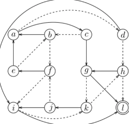
Figure 3 shows an example of a network of twelve nodes. The elementary cycles are:C1= (a, c, b, a), C2= (b, f, e, b), C3 = (g, k, h, g), C4 = (i, k, j, i), C5 = (f, i, k, j, f ), C6 = (a, c, b, f, e, a), C7 = (a, c, g, k, j, f, e, a), C8 = (a, d, i, k, j, f, e, a), C9 = (a, c, g, k, j, f, e, b, a), C10 = (a, d, h, g, k, j, f, e, a), C11 = (a, d, i, k, j, f, e, b, a), and C12= (a, d, h, g, k, j, f, e, b, a). It is possible to compute the nodes that break each cycle. We obtain{c} for C1,{b, e} for C2,{g, k} for C3,{i} for C4,{f, i} for C5,{c} for C6,{g, j} forC7,{a, i, j} for C8,{e, g, j} for C9,{a, d, g, j} for C10, {a, e, i, j} for C11, and{a, d, e, g, j} for C12. Cycles that are broken by only one node are C1,C4 and C6. Thus, nodes c andi are added to S. Note that these nodes also break cycles C5,C8 andC11, which do not need to be broken by another node. Then, the node that breaks the most cycles is g (as it breaks five of the remaining cyclesC3,C7,C9,C10andC12), so g is added to S. With S = {c, g, i}, only C2 remains.
Algorithm 1: Computation of the nodes that break all cycles in ACH.
Data:SCC is a strongly connected component, R1 and R2 are routing protocols
Result: list of nodes fromSCC that perform the transition in the same step
S ← ∅;
for each cycleC in elementary cycles of SCC do for eachn ∈ C do
ifR1(n) /∈ C then n breaks C; end
end
ifC is broken by only one node then addn to S;
end end repeat
n ←the node of SCC \ S that breaks the most unbroken cycles;
addn to S;
until every cycle is broken by a node ofS; returnSCC \ S
Both b and e can break C2, so b is chosen arbitrarily. The resulting setS is {b, c, g, i}, and the nodes that can perform the transition during the first step are{a, d, e, f, h, j, k, l}. For the second step, ACH considers that all nodes of the first step route according to R2 (that is,R1 ← R2), and reapplies the same algorithm. The second step is thus{b, c, g, i}.
B. ACH for multiple destinations
ACH operates as follows when there are multiple des-tinations. It first computes the steps for each destination independently (see Algorithm 1). Then, it merges the steps for all destinations. Let us denote bystep(i, j) the set of nodes of thei-th step of ACH for the single destination j. Then, the i-th step of ACH for all destinations is computed by merging the i-th step of each destination, that is step(i) = ∪d
j=1step(i, j), whered is the number of destinations.
Figure 1 showed an example of a network of five nodes {a, b, c, d, e} with three destinations {a, d, e}. When con-sidering destinations independently, ACH produces steps ({a, d, e}, {c}, {b}) for destination a, ({a, d, e}, {b}, {c}) for
a b c d
e f g h
i j k l
Figure 3. A small network with twelve nodes and eleven elementary cycles, used as an example for ACH.
destination d, and ({d, e}, {c}, {b}, {a}) for destination e. When merging the steps, ACH produces the following four steps ({d, e}ade∪ {a}ad, {c}ae∪ {b}d, {b}ae ∪ {c}d, {a}e). Recall that on this network, RTH-p produced seven steps and SCH-p produced ten steps.
It can be noticed that the number of steps produced by ACH does not depend on the number of nodes of the network, nor on the number of destinations (as they are all merged by ACH). The number of steps produced by ACH depends on the largest number of steps for a single destination. Thus, the transition duration isO(1). The computation cost of ACH is larger with ACH than with RTH, RTH-p and SCH-p. However, we believe that it is more important for the transition to be fast than for the computation of the transition to be fast, as the computation can be done off-line.
IV. SIMULATIONRESULTS
In this section, we compare the performance of our heuristic ACH with two other heuristics from the literature: RTH-p (which is an improvement of RTH) and SCH-p.
A. Performance metrics
The number of groups of compatible destinations indicates how a heuristic handles multiple destinations. A group of compatible destinations is the set of destinations which are treated together by a heuristic. For RTH-p, it is equal tot + 1, where t is the number of troublesome destinations (and 1 represents the set of all non-troublesome destinations, which are treated together). For SCH-p, it is equal to d, where d is the number of destinations, because each destination is treated independently. For ACH, it is equal to 1, because all destinations are treated together. This metric is mainly used to better understand the results of the other metrics.
The duration of the transition is our main metric, and it is computed as the overall number of steps of the transition. Here, we assume that one step corresponds to a time unit, as all nodes can be configured in parallel and can perform the transition in arbitrary order. The smaller is the number of steps, the faster is the transition.
The cost of the transition is the number of control messages required to perform the transition. It is equal to the sum of the number of distinct nodes per step, as each node has to be configured independently at each step where it appears. For example, for the transition ({d, e}ae, {c}ae, {b}ae, {a}ae, {a, d, e}d, {b}d, {c}d), the first step generates two messages (for d and e, independently of the fact that two destinations are involved), the second one message (forc), the third one message (for b), the fourth one message (fora), the fifth three messages (for a, d and e), the sixth one message (for b) and the seventh one message (for c). The cost of the transition is thus ten.
B. Simulation settings
Our simulations are performed on random connected net-work graphs of size varying from50 to 200 nodes. Nodes are deployed uniformly at random in an area of 100 m×100 m. The communication range of nodes is set to 20 m (which is a standard setup for wireless adhoc networks). We considered that each node is a potential destination. For each destinationd, we generatedRd
1by assigning a random weight within[1; 100] to each link, and by computing the shortest path from each node tod using these weights. Similarly, we generated Rd
2 by assigning a random weight within[1; 50] to each link, and by computing the shortest path from each node to d using these weights. Simulations are repeated 100 times, and a confidence interval of 95% is shown on plots.
C. Results
In the following, we present and analyze our simulation results on our three metrics. Note that all plots are shown with a logarithmic scale for the y-axis.
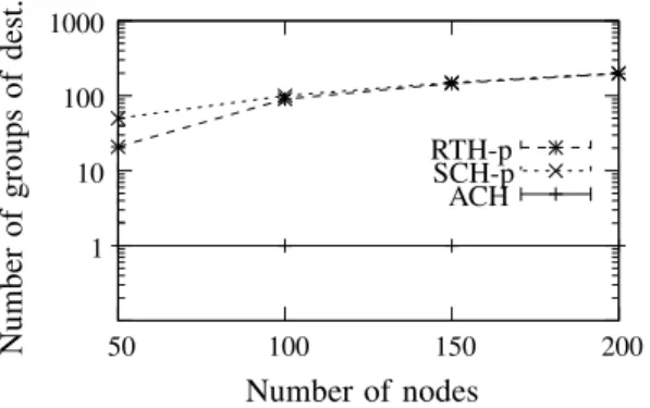
1) Number of groups of compatible destinations: Figure 4 shows the average number of groups of compatible destina-tions, for varying network sizes and for the three heuristics RTH-p, SCH-p and ACH. For ACH, the number of groups of compatible destinations is always one because ACH considers all destinations together. For SCH-p, this number is equal to the number of destinationsd (which is equal to the network size in our settings), because SCH-p considers all destinations independently. For RTH-p, this number is between 1 and d. For networks of 50 nodes, nearly 30 destinations are non-troublesome (which allows RTH-p to consider only 21 groups of destinations: one for the 30 non-troublesome destinations, and 20 for the remaining 20 troublesome destinations). How-ever, as the network size increases, non-troublesome destina-tions become less frequent. For networks of 200 nodes, only 3 destinations on average are non-troublesome.
2) Duration of the transition: Figure 5 shows the duration of the transition, computed as the average number of steps required to perform the transition for all destinations, for varying network sizes. We notice that the number of steps increases consistently with the size of the network for both RTH-p and SCH-p heuristics. For RTH-p, this is due to two factors: the increase in the number of groups of compatible destinations (see Figure 4), and the increase in the number
1 10 100 1000 50 100 150 200 Number of nodes N u m b er o f g ro u p s o f d es t. RTH-p SCH-p ACH
Figure 4. Number of groups of compatible destinations as a function of the number of nodes, for the three heuristics.
of steps for each destination (due to the fact that the number of steps for each destination in RTH-p is equal to depth of the routing tree Rd
2). For SCH-p, this is due to the increase in the number of destinations, as destinations are treated separately. ACH, however, is able to produce a very small number of steps, independently of both the number of nodes and the number of destinations, as its number of steps is equal to the maximum number of steps for every destination. ACH outperforms RTH-p with a gain varying from 98% for small networks up to 99% for large networks. Likewise, ACH outperforms SCH-p with a gain varying from 97% for small networks up to 99% for large networks. It is also important to note that, out of the 400 simulation results we obtained, ACH reached a maximum of 6 steps only once, and 5 steps or less for all the remaining simulations.
1 10 100 1000 10000 50 100 150 200 Number of nodes N u m b er o f st ep s RTH-p SCH-p ACH
Figure 5. Duration of the transition as a function of the number of nodes. It can be seen that the duration of the transition for ACH does not increase with the number of nodes nor with the number of destinations.
3) Cost of the transition: Figure 6 shows the cost of the transition, computed as the average number of control messages required to perform the transition for all destinations. For all heuristics, the number of control messages increases with the network size, as more nodes have to be configured overall. For large networks, RTH-p and SCH-p achieve similar results, which comes from the fact that these two heuristics are unable to merge destinations. The number of control messages is equal to n.d for SCH-p. For ACH, the small control overhead comes from the fact that all steps are merged: when a node appears several times in the same step for different destinations, it is counted only once as a single
control message can configure the transition of this node for all destinations. In networks of 50 nodes, ACH outperforms RTH-p with a gain of 94%, and SCH-p with a gain of 97%. In networks of 200 nodes, the gain of ACH is 99% compared to both RTH-p and SCH-p. 10 100 1000 10000 100000 50 100 150 200 Number of nodes N u m b er o f co n tr o l m es sa g es RTH-p SCH-p ACH
Figure 6. Cost of the transition as a function of the number of nodes, for the three heuristics. Due to a small number of steps, ACH is able to perform the transition for all destinations with a limited overhead.
V. CONCLUSION
The transition from one routing protocol to another routing protocol can lead to transient routing loops in networks. In this paper, we propose a fast loop-free transition algorithm called ACH. ACH focuses on identifying a small set of nodes that break cycles in strongly connected components, in order to ensure that many nodes can perform the transition in parallel, which reduces the overall transition duration. Compared to the main heuristics of the literature RTH-p and SCH-p, our simulation results on random networks show that ACH out-performs both of them. In term of the number of steps, the gain of ACH compared to RTH-p varies from 98% (for small networks) to 99% (for large networks), and the gain compared to SCH-p varies from 97% (for small networks) to 99% (for large networks). In term of the number of control messages, the gain of ACH compared to RTH-p varies from 94% (for small networks) to 99% (for large networks), and the gain compared to SCH-p varies from 97% to 99%.
ACKNOWLEDGMENT
This work has been sponsored by the French govern-ment research program ”Investissegovern-ments d’avenir” through the IMobS3 Laboratory of Excellence (ANR-10-LABX-16-01), by the European Union through the regional program competitive-ness and employment 2014-2020 (ERDF - Auvergne region), and by the Auvergne region.
REFERENCES
[1] K. Butler, T. R. Farley, P. McDaniel, and J. Rexford, “A survey of BGP security issues and solutions,” Proceedings of the IEEE, vol. 98, no. 1, pp. 100–122, 2010.
[2] Z. Zhong, R. Keralapura, S. Nelakuditi, Y. Yu, J. Wang, C. N. Chuah, and S. Lee, “Avoiding transient loops through interface-specific forwarding,” in IEEE/ACM IWQoS (International Symposium on Quality of Service),
ser. Lecture Notes in Computer Science, vol. 3552. Springer, 2005, pp.
[3] P. Francois and O. Bonaventure, “Avoiding transient loops during the convergence of link-state routing protocols,” IEEE/ACM Transactions on
Networking, vol. 15, no. 6, pp. 1280–1292, Dec 2007.
[4] S. Nelakuditi, Z. Zhong, J. Wang, R. Keralapura, and C. N. Chuah, “Mit-igating transient loops through interface-specific forwarding,” Computer
Networks, vol. 52, no. 3, pp. 593–609, 2008.
[5] L. Le Guennec, N. El Rachkidy, A. Guitton, M. Misson, and K. Kelfoun, “MAC protocol for volcano monitoring using a wireless sensor network,” in NoF (International Conference on Network of the Future), 2015. [6] L. Vanbever, S. Vissichio, C. Pelsser, P. Francois, and O. Bonaventure,
“Lossless migrations of link-state IGPs,” IEEE/ACM Transactions on
Networking, vol. 20, no. 6, pp. 1842–1855, 2012.
[7] N. El Rachkidy and A. Guitton, “Changing the routing protocol without transient loops,” Computer Communications, 2016, to appear.
[8] D. B. Johnson, “Finding all the elementary circuits of a directed graph,”
![Figure 1. Example from [7] of routing protocols for three destinations: (a) a is the destination, (b) d is the destination, and (c) e is the destination.](https://thumb-eu.123doks.com/thumbv2/123doknet/14368851.504019/4.918.103.812.74.210/figure-example-routing-protocols-destinations-destination-destination-destination.webp)