HAL Id: hal-02052183
https://hal.archives-ouvertes.fr/hal-02052183
Submitted on 28 Feb 2019
HAL is a multi-disciplinary open access
archive for the deposit and dissemination of
sci-entific research documents, whether they are
pub-lished or not. The documents may come from
teaching and research institutions in France or
abroad, or from public or private research centers.
L’archive ouverte pluridisciplinaire HAL, est
destinée au dépôt et à la diffusion de documents
scientifiques de niveau recherche, publiés ou non,
émanant des établissements d’enseignement et de
recherche français ou étrangers, des laboratoires
publics ou privés.
Power alternator simulation models for diagnostic
purposes
Clément Filleau, Jacques Saint-Michel, Emile Mouni, Antoine Picot, Pascal
Maussion
To cite this version:
Clément Filleau, Jacques Saint-Michel, Emile Mouni, Antoine Picot, Pascal Maussion. Power
alterna-tor simulation models for diagnostic purposes. Mathematics and Computers in Simulation, Elsevier,
2019, 158, pp.281-295. �10.1016/j.matcom.2018.09.013�. �hal-02052183�
OATAO is an open access repository that collects the work of Toulouse
researchers and makes it freely available over the web where possible
Any correspondence concerning this service should be sent
to the repository administrator:
[email protected]
This is an author’s version published in:
http://oatao.univ-toulouse.fr/21458
To cite this version:
Filleau, Clément and Saint-Michel, Jacques and Mouni, Emile
and Picot, Antoine and Maussion, Pascal Power alternator
simulation models for diagnostic purposes. (2019)
Mathematics and Computers in Simulation, 158. 281-295.
ISSN 0378-4754
Official URL:
https://doi.org/10.1016/j.matcom.2018.09.013
Fig. 1. Simulink dq-model of a self-excited alternator.
The modelling of synchronous machines immediately evokes dq-models,Fig. 1. These models have become a globalised standard in machine modelling, whether for induction machines [2,3], synchronous machines [11,7] or self-excited power alternators [8,10]. They are compact, quite easy to develop, and highly efficient for machine control. Nevertheless, this kind of model may not be suitable for diagnoses. Indeed, dq-models are a sort of “mean-value” models that allow an efficient control of the output voltage [1], and can be relatively inaccurate and simplistic when dealing with precise spectral calculations in self-excited alternators. Since machine diagnostic methods are often based on spectral analysis [9], new modelling strategies are needed to obtain accurate spectra. Finite element modelling can be used to accurately take into account all geometrical and magnetic effects in the machine. However, as will be discussed in this paper, their complexity and computational time are problematic and render them impractical for diagnostic purposes. In this paper a new modelling method for salient-pole power alternators by means of a process mixing finite element and analytical simulations is presented. It is based on a co-simulation process between finite elements and a state model. It is demonstrated that, compared with dq-models, such a method leads to more precise spectra, closer to experimental ones, for all the currents and voltages in the system. This characteristic is a huge advantage given that most of the diagnostic methods are currently based on spectral signature analysis in electrical signals.
The second section presents both the dq-model and the new co-simulation method. A brief description of the differential equations used in the two models and the use of finite elements in the new one are depicted as well as crucial specificities regarding this type of modelling. Section 3 presents a validation of the Flux2D/Matlab model results thanks to a finite element simulation before concentrating on a global comparison of simulated and experimental results for dq and Flux2D/Matlab models. This model was also presented in [5]. The fourth section deals with evaluation. Results are discussed from a diagnostic perspective. Section5presents the improvements obtained with the new approach and a conclusion discusses the advantages, limitations and perspectives of this study.
2. Power alternator modelling 2.1. DQ models
As already mentioned in the introduction, dq-models of electrical machines may be viewed as “mean-value-models”, particularly suitable for control purposes.
Indeed, voltage control needs a good representation of the generator dynamics and output voltage magnitude. An efficient controller, capable of maintaining its mean square root value constant whatever disturbance occurs, may thereby be designed. To validate our approach, a basic dq-model of the complete system has been developed in Matlab-Simulink environment. It is composed of two dq-models: one for the exciter and for the generator; a rotating
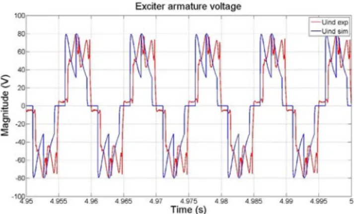
Fig. 2. Experimental (red) dq-model and simulated (blue) exciter armature voltage at nominal operating point (tsim=5 s, fs=100 kHz). (For
interpretation of the references to colour in this figure legend, the reader is referred to the web version of this article.)
full-wave rectifier with six diodes rectifying the three-phase voltage produced by the exciter in order to supply the field of the main generator and a parallel RL output load. Both exciter and generator models are composed of a set of two space–state equations and adequate dq0/123 transformations that ensure the connection to the rest of the circuit. The state–space equations implemented in the model are given in(1).
˙ X = AX + BU (1) With X = [Id Iq I0If IDIQ] State-space vector Id Iq I0 dq0 output currents If Field current
ID D-axis damper current
IQ Q-axis damper current
A Dynamic matrix B Input matrix U =[ vdvqv0vf vDvQ ] Input vector
The parameters of the two machines come from experimental identification tests performed on a 27 kVA alternator provided by Leroy Somer.Fig. 2presents a temporal comparison of the exciter armature voltage Uind between the
experimental measurements (blue) and the simulation results obtained with a dq-model (red). The excitation voltage of the model is set so that a 400 V rms output voltage is produced at nominal operating point (power factor 0.8). Experimental measurements were also performed at the nominal operating point of the alternator. Both signals are sampled at 100 kHz a 5 s period in order to leave enough time for the transient effects to damp out. It is obvious from
Fig. 2that the simulated signal (blue) lacks accuracy compared to the experimental one (red). 2.2. Flux2D/Matlab co-simulation principles
In order to improve the signal modelling of the whole system, a precise analytical description of the entire system (exciter, rectifier, generator and output loads) was developed. The differential equations obtained for the two rotating machines involve the three-phase self and mutual inductances. Unlike dq-inductances, the three-phase inductances are not constant but evolve as a non-perfectly sinusoidal wave all along the air gap due to the mechanical geometry and imperfections of the machine. The imperfections are both the main problem and the main characteristic that must be taken into account if accurate waveforms are to be expected. A finite element simulation is needed to obtain a true inductance repartition along the air gap for each coil by taking into account the exact topology of the machine. This is computed with Flux2D.
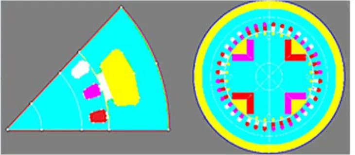
Fig. 3. Geometrical and physical description of the exciter (left) and the alternator (right).
Unfortunately, it is impossible to calculate general inductances that are suitable for all functioning states of the generator. Inductances are very sensitive to magnetic saturation and, given that generators operate mainly around the inflexion point of the magnetic saturation curve of the materials, their magnitude will always be affected by the saturation level of the generator. In addition, magnetic saturation is a local phenomenon that has different impacts with regard to the angular position of the rotor and it cannot be taken into account as a global attenuation of the signals’ waveforms. This is less true for the exciter that mainly operates in the linear part of the saturation curve. To avoid a complexity explosion with, e.g. the use of inductance tables for each operating point, this study was limited to the linear world. It is therefore evident that simulation results could differ in terms of magnitude. However, what is expected is a global match between simulated and experimental waveforms, and thereby harmonic representations of the system, so that comparisons between healthy and faulty spectra become feasible. The proposed approach is described in the following sections.
2.2.1. Inductance identification in FLUX2D Geometrical description
A thorough geometrical description of the exciter and the alternator was elaborated in Flux2D in accordance with the mechanical plans delivered by Leroy-Somer. Both machines are salient pole models with four and two pole pairs respectively. Therefore, considering the geometrical symmetries in rotating machines, only an eighth of the exciter and a quarter of the alternator have to be modelled in order to obtain their complete behaviour. Nevertheless, the ultimate goal of this model is to study the impact of electrical faults located in the alternator on the system signals. These faults may be non-symmetrical, such as local inter-turn short-circuits. Consequently, the alternator has to be modelled all along the air gap (as inFig. 3). The disposition of the coils in the main machine is a 2/3 step repartition with two times two parallel windings of 48 turns each mounted in series for each phase, so that the desired 400 V output voltage can be reached. Field coil has 82 turns/pole.
Physical description
Given that the desired inductances are taken as linear, there is no need to describe the saturation curve of the magnetic materials in the machines. A single magnetic material is considered for the whole system, (magnetic permeabilityµr = 10.000). Each material with different electrical and magnetic properties is represented with a
different colour inFig. 3. Electrical description
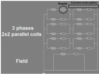
In parallel to the spatial description, an electrical circuit depicting the operational conditions of the machine has to be developed. It controls the polarity of the flowing currents, the parameters of each coil, the supply of the field and the load as seen inFig. 4.
Meshing
The aim of Flux2D simulations only consists in the calculation of inductance waveforms. It does not require a particularly fine meshing. Consequently, automatic meshing is satisfactory to obtain smooth inductance waveforms.
Fig. 4. Electrical circuit for identification purposes.
Identification
The identification of the inductances consists in making a 1 A current flow through one single coil of the machine and to measure the flux circulating in this coil and the others. That way, the self-inductance of the supplied coil and the mutual inductances with all the others can be obtained.
Given thatϕ = Li, the flux generated by a 1 A current is directly equivalent to the inductance value. In order to avoid distorting the waveforms, only one coil has to be supplied and the current in all the other coils must imperatively be blocked. This operation is achieved by means of high resistances (1 G) in series with each non-supplied coil and by an escape path to the ground for the circulating current (lower part ofFig. 4). Failure to do this would generate an undesired current flow through another coil of the machine and create another circulating flux in the magnetic circuit, thereby distorting the inductances that have been identified.
It would seem simpler to define a mechanical sampling of 1◦, in order to obtain the spatial repartition of the flux
in each coil all around the air gap. In fact, such a mechanical step introduces a non-finite time step of 1/9 ms and therefore leads the software to compute undesired approximations. This may appear to be a detail but can be the cause of significant problems in the next step of the simulation, in particular the decomposition of the inductances in the Fourier series. This step is essential to reconstruct all the inductances and their derivatives at the sampling rate used in the Matlab algorithm.
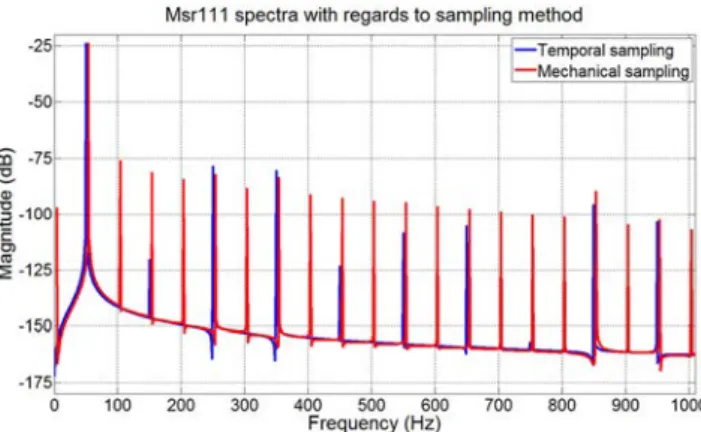
Using mechanical sampling in Flux2D produces resulting data samples that are not well distributed over time, creating undesired harmonics when applying decomposition in the Fourier series based on a fixed time step.Fig. 5
shows the harmonic contents of a rotor-stator phase 111 mutual inductance sampled by means of mechanical (red) and temporal (blue) steps.
These inductance harmonics disturb in turn the waveforms of the simulated electrical signals. In order to remedy this, the mechanical step was discarded and replaced by a fixed time step of 0.1 ms for all identifications. This sampling time is in accordance with the original value of 1/9 ms corresponding to one mechanical degree when the mechanical rotation speed of the rotor is 25 Hz. Thus, an integer number of points over one rotor turn can be calculated. The duration of the identification was set to 60 ms in order to allow 20 ms for the alternator to recover from any eventual transient phenomenon at the beginning of the simulation, still obtaining the behaviour of the inductances on a whole rotor turn (40 ms at 25 Hz). At the end of the identification process, a thorough representation of the interactions between the fluxes in the machine is obtained through the self and mutual inductances, additionally including the mechanical features of the alternator.
Fig. 5. Spectra of the mutual inductance between rotor and stator phase 111 sampled with mechanical (1◦, red) and temporal (0.1 ms, blue) steps.
(For interpretation of the references to colour in this figure legend, the reader is referred to the web version of this article.)
Fig. 6. Electrical equivalent circuit of the exciter.
2.2.2. Analytical simulation in MATLAB
Matlab is used to obtain an analytical description of the system by means of differential equations. The currents circulating through the two rotating machines are the model state variables. To avoid redundancy, only the exact number of state variables accurately describing the system was considered in the main equations presented below.
•Exciter model
The exciter inFig. 6is fully described by three equations. Expressions(2)and(3)depict the inter-phase relations and(4)the inductor behaviour. More precisely, the first two equations are functions of the exciter phase currents Ix
and inductances Lx, of the currents jx and on-state resistances rx of the three-phase rectifier and of the excitation
current Iex c. With a star connection without neutral, the third phase current is expressed as a combination of the other
two. d(ϕ1−ϕ2) dt = −Rphe. f (Ix) + f (Ix, Lx, jx, rx, Iex c) (2) d(ϕ2−ϕ3) dt = −Rphe. f (Ix) + f (Ix, Lx, jx, rx, Iex c) (3) dϕex c dt =uex c−Rexc.iex c (4)
•Diode rectifier model
Fig. 7presents the rectifier circuit setup in the rotor. The rectifier does not deal with energy transfers and has consequently no own state variables. Currents flowing through and voltage at the terminals of the rectifier are fixed by their environment. Three intermediate variables j1, j2 (currents in the rectifier) and urp(alternator field voltage)
Fig. 7. Electrical equivalent circuit of the rectifier.
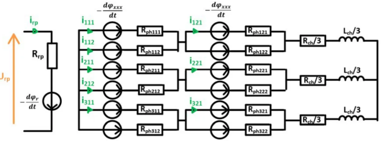
Fig. 8. Electrical equivalent circuit of the alternator.
are thus calculated with regard to diode on-state resistances rx, input currents Ix, output current Ir pas well as rectifier
currents jx.
•Alternator model
The alternator model inFig. 8is described by nine equations. Expressions(5)and(6)consider the global inter-phase relations,(7)to(12)describe the relationship between the parallel coils in each phase and(13)deals with the alternator field current. Alternator phase currents Ix are functions of state variables ix, the currents in each parallel
coil. The variables not indicated inFig. 8are fully described by combinations of other state variables.
d( f (ϕx)) dt + Lch 3 d( f (ix)) dt = −Rphx. f (ix) − Rch 3 f(ix) (5) d( f (ϕx)) dt + Lch 3 d( f (ix)) dt = −Rphx. f (ix) − Rch 3 f(ix) (6) d(ϕ111−ϕ112) dt = −Rph111i111−Rph112i112 (7) d(ϕ121−ϕ122) dt = −Rph121i121−Rph122i122 (8)
d(ϕ211−ϕ212) dt = −Rph211i211−Rph212i212 (9) d(ϕ221−ϕ222) dt = −Rph221i221−Rph222i222 (10) d(ϕ311−ϕ312) dt = −Rph311i311−Rph312i312 (11) d(ϕ321−ϕ322) dt = −Rph321i321−Rph322i322 (12) dϕr p dt =ur p−Rrp.Ir p (13) •General algorithm
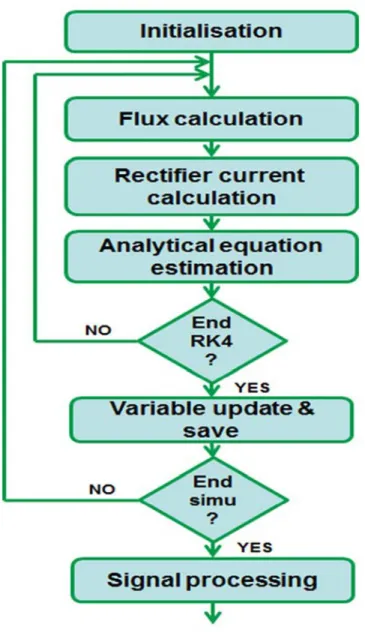
After an initialisation phase for all variables, a temporal loop dependant on the total simulation time begins. For each time step, the ongoing values of the inductances are determined in order to calculate the values of the state variable derivatives. The programme then integrates all those variables by means of a Runge Kutta 4 process and, obtaining the values of the state variables themselves, is able to determine every voltage, current and flux in the two machines. The algorithm of this programme is presented inFig. 9.
2.3. Flux2D model
The final modelling method that may be considered originates in the finite elements themselves. The geometrical model of the alternator created in Flux2D may be used as a whole in order to perform very accurate simulations. This has the great advantage of taking into account every minute detail that may influence the waveforms of the simulated electrical signals: geometry, electric phenomenon and magnetic saturation. It also has the capacity to adapt itself to every configuration that is required by the user, thus allowing fine fault modelling which is particularly useful for diagnostic applications.
3. Results
3.1. Comparison between finite element and Flux2D/Matlab model
The advantage of finite elements is that they take into account the magnetic saturation in the machine. Nonetheless, this approach is not well suited to model such a system. Two alternators mechanically coupled and electrically connected through the three-phase rectifier are not easy to represent in the software. Only one machine can be simulated at a time and as a matter of fact, the field voltage supplying the alternator can either be fixed as constant or as a rectified sinusoidal three-phase voltage. In both cases, it will not be harmonically as rich as the real field voltage from the exciter armature and a loss in accuracy will be inevitable. In addition, the calculation time for such a model is incompatible with diagnostic applications that require a large number of simulations to obtain comprehensive databases for each fault. That is why the finite element model used in this section to compare the results is in fact very close to that of the Flux2D/Matlab in that it is composed of linear materials in order to validate the accuracy of the proposed model. To evaluate the incompatibility of such a finite element model with a diagnostic approach, equivalent simulations were undertaken with finite elements and Flux2D/Matlab models. The first takes four times longer than the second, keeping in mind that it was performed with a time step a thousand times bigger and with no magnetic saturation. This demonstrates one of the main advantages of the proposed approach.
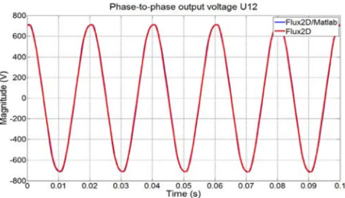
Figs. 10and11present the waveforms of the alternator armature voltage and the electromotive force measured at the terminals of the H1 auxiliary winding at nominal operating point with finite elements (red) and Flux2D/Matlab modelling (blue). Given the lack of exciter in the finite elements model, both simulations were performed by directly supplying the field of the alternator with a constant voltage of 22 V.
The results obtained prove that thanks to the identified inductances, the proposed approach performs as well as the finite elements and that the same level of accuracy in the signal waveforms can be expected with no disadvantages listed in this section. A faster and more user-friendly model should be attainable without losing the precision that is needed to adequately simulate the faults of the alternator.
Fig. 9. Algorithm for analytical equations identification.
3.2. Comparison between DQ and Flux2D/Matlab model
To confirm the improvement in signal waveforms,Fig. 12 depicts a temporal comparison of exciter armature voltage between measured and simulation results from the Flux2D/Matlab model at the nominal operating point (400 V output voltage and PF = 0.8).
Fig. 12indicates a clear improvement has been made compared to dq-model results inFig. 2. In order to evaluate the improvements of the proposed method, a spectral presentation of the main signals of the system is depicted in
Figs. 13to16. In each figure, the experimental spectra are depicted in red (upper part), the one simulated with the dq-model in blue in the middle part, and the one simulated with the proposed approach in green (lower part). These signals are the exciter and alternator field current Iexc(Figs. 13and15) and armature voltages Uindand U12(Figs. 14
and16). Each data set, either simulated or experimental, consists of a 1 s signal sampled at 100 kHz. The three spectra of each signal are artificially shifted by 6 Hz for better legibility. Particular care has been taken regarding the steadiness of the signals before performing the FFT.
Fig. 10. Finite elements (red) and Flux2D/Matlab (blue) simulated main generator armature voltages U12at nominal operating point (tsim=0.1 s,
fs=100 kHz, Urp=22 V). (For interpretation of the references to colour in this figure legend, the reader is referred to the web version of this
article.)
Fig. 11. Finite elements (red) and Flux2D/Matlab (blue) simulated auxiliary winding H1 electromotive force at nominal operating point (tsim = 0.1 s, fs = 100 kHz, Urp = 22 V). (For interpretation of the references to colour in this figure legend, the reader is referred to the web version of this article.)
Fig. 12. Experimental (red) and Flux2D/Matlab simulated (green) exciter armature voltage at nominal operating point (tsim=0.1 s, fs=100 kHz).
(For interpretation of the references to colour in this figure legend, the reader is referred to the web version of this article.)
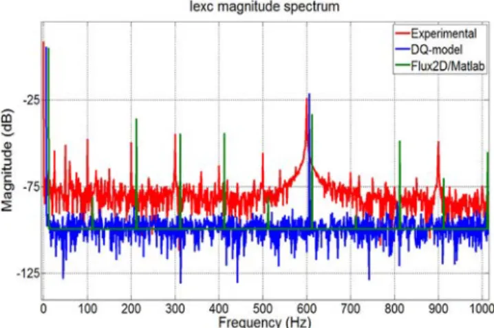
The analysis ofFigs. 13to16shows that the harmonic contents of the dq-model signals are only composed of the main harmonics and are thus very poor compared to experimental measurements. Given that most of the diagnostic methods are based on the detection of spectral signatures [9], those results might not be suitable for diagnostic
Fig. 13. Spectral contents of experimental, dq- and Flux2D/Matlab-simulated exciter field currents Iexc(tsim=1 s, fs=100 kHz, artificial
shifting).
Fig. 14. Spectral contents of experimental, dq- and Flux2D/Matlab-simulated exciter armature voltages Uind(tsim=1 s, fs=100 kHz, artificial
shifting).
Fig. 15. Spectral contents of experimental, dq- and Flux2D/Matlab-simulated main generator field currents Irp(tsim=1 s, fs=100 kHz, artificial
Fig. 16. Spectral contents of experimental, dq- and Flux2D/Matlab-simulated main generator armature voltages U12(tsim=1 s, fs=100 kHz,
artificial shifting).
Table 1
DQ, finite elements (FE) and Flux2D/Matlab (F/M) computation time ratios.
Model DQ FE F/M
Time 1 140 000 35
purposes. On the contrary, there is a clear improvement of the signals from the proposed method in terms of spectral content. A far more complete harmonic representation is obtained through a fine description of machine inductances. Despite the expected magnitude differences, the quality of the simulated signals is such that the impacts of electrical faults on harmonics can be studied.
This enhanced accuracy comes at a cost. The Flux2D/Matlab model takes thirty-five times longer to compute than the dq-model with equivalent simulation parameters and excluding the identification process that is set once and for all. Nevertheless, the code which has been developed is still approximate and an optimisation process could certainly decrease this computation time.Table 1gives an idea of the ratio between computation times of dq, finite elements and Flux2D/Matlab models, considering the dq-model as a reference.
4. Evaluation and discussion
To evaluate the improvement obtained with the new model, an error calculation between experimental and simulated spectra was set up. It consists in calculating the absolute errors between the different harmonic families: multiples of 100 Hz for the currents and the exciter armature voltage and uneven multiples of 50 Hz for the alternator armature voltage. To avoid large gaps between the different errors for each component, the latter are pictured along a logarithmic scale.Figs. 17to20depict the absolute spectral errors with the experimental spectra. The new method is plotted in green and the dq-model in red.
Table 2shows the results for average, minimal and maximal errors. The analysis ofTable 2confirms the remarks made inFigs. 17to20. The Flux2D/Matlab model provides more accurate spectral representations than the dq-model e.g., the mean errors have decreased from 46.8 dB to 33.3 dB for Iexcand from 37.5 to 18.1 for Uind. Error values are
due to the fact that it is not possible to estimate the correct amplitude value of the signals, as mentioned in Section2. Nonetheless, the proposed method provides an accurate representation of the spectral content of the different signals. The last line ofTable 2displays the average errors of the four considered signals, and indicates that a valuable global improvement is achieved on the average errors. The minimal and maximal errors also decrease but the significance of this result is not particularly meaningful for the stated aim of this modelling. The global improvement in the spectral contents of the electrical signals is a valuable feature for developing more precise diagnostic methods on the basis of the simulations. So, this model is more appropriate to study the harmonic behaviour of the system when faults occur and is a first step towards the design of relevant indicators for system monitoring.
Fig. 17. Absolute error for exciter field current Iexcbetween experimental and Flux2D/Matlab results (green) and experimental and dq-model (red).
(For interpretation of the references to colour in this figure legend, the reader is referred to the web version of this article.)
Fig. 18. Absolute error for exciter voltage Uindbetween experimental and Flux2D/Matlab results (green) and experimental and dq-model (red).
(For interpretation of the references to colour in this figure legend, the reader is referred to the web version of this article.)
Fig. 19. Absolute error for alternator field current Irpbetween experimental and Flux2D/Matlab results (green) and experimental and dq-model
Fig. 20. Absolute error for alternator voltage U12between experimental and Flux2D/Matlab results (green) and experimental and dq-model (red).
(For interpretation of the references to colour in this figure legend, the reader is referred to the web version of this article.)
Table 2
Experimental and simulated harmonic errors: Flux2D/Matlab (F/M) vs. dq (DQ) models. Signal Model F/M DQ Iexc 33.3 (0.1–66.4) 46.8 (5.2–93.3) Uind 18.1 (1.9–119.4) 37.5 (1.7–82.5) Irp 52.2 (2.7–108.4) 104.7 (0.6–160.4) U12 21.2 (0.5–97.9) 36.0 (0.3–96.9) Average 31.2 (1.3–98.0) 56.3 (2.0–108.3)
5. Limitations, perspectives and conclusion
Even if dq modelling is very accurate for the control of a system, it has been shown in this paper that the corresponding model was rather limited in terms of harmonic representation. The original co-simulation process proposed in this paper is a valuable tool for the diagnosis of salient pole synchronous generators, since it provides more accurate spectral representations. Despite the limitation within a linear world, the waveforms obtained are sufficiently precise for an accurate spectral study. The linearity issue may accentuate the impact of faults on harmonic magnitudes but it is still possible to predict which spectral component may turn out to be a valuable default indicator. In addition, a simulation with this model on an Icore3 computer is easier to use, has finer simulation steps and is far quicker than an equivalent simulation executed by means of finite elements on an Icore7 computer.
Analytical models, subject to improvements such as mechanical dynamic introduction, might also be used for control design, but only for specific precision requests, as the global method is more time consuming than dq-modelling. Indeed, finite element simulations require precise handling; even the smallest error in inductance identifications may lead to disastrous results because they derive from the discretization of the differential equations of the system in Flux2D.
The next step is to use this method to study the spectral behaviour of the system for different kinds of faults and to confront it with experiments to check the relevancy of the proposed approach in terms of diagnosis. This has already been undertaken and promising results are published in [4].
Acknowledgements
The authors would like to sincerely thank Mr. Sundara Khamfonh and Mr. Laurent Rouyer from Leroy Somer for their invaluable help in setting up the experimental test bench, as well as Mr. ´Emile Mouni, Mr. Jacques Saint-Michel, Mr. Phillipe Manf´e and Mr. Xavier Jannot for their technical advice. This work was funded by Leroy Somer and the ANRT, Agence Nationale de la Recherche et de la Technologie.
References
[1] A. Barakat, S. Tnani, G. Champenois, E. Mouni, Monovariable and multivariable voltage regulator design for a synchronous generator modeled with fixed and variable loads, IEEE Trans. Energy Conv. (2011).
[2] R.E. Betz, R.J. Evans, Torque, Speed and position control of induction machines using the DQ Model, in: Technical Report EE8503, Electrical and Computer Eng. Dept, Univ of Newcastle, 1985.
[3] C. Dufour, S. Cense, J. Bélanger, An induction machine and power electronic test system on FPGA, in: ELECTRIMACS 2014, 2014, Spain. [4] C. Filleau, A. Picot, P. Maussion, P. Manfé, X. Jannot, Stator short-circuit diagnosis in power alternators based on Flux2D/Matlab co-simulation, in: Presented At the 11th IEEE International Symposium on Diagnostics for Electric Machines, Power Electronics and Drives (SDEMPED), 2017.
[5] C. Filleau, J. Saint-Michel, E. Mouni, A. Picot, P. Maussion, Fine power alternator modelling for diagnosis purposes by means of Flux2D/Matlab co-simulation, in: Presented at the ELECTRIMACS Conference, 2017.
[6] M. Li, H. Xiao, W. Gao, L. Li, Smart grid supports the future intelligent city development, in: Chinese Control and Decision Conference, 2016.
[7] R. Mbayed, G. Salloum, L. Vido, E. Monmasson, M. Gabsi, Hybrid excitation synchronous generator in embedded applications: modelling and control, in: Mathematics and Computers in Simulation 90, IMACS, 2012.
[8] E. Mouni, S. Tnani, G. Champenois, Synchronous generator output voltage real-time feedback control via H∞ strategy, IEEE Trans. Energy Convers. 24 (2) (2009).
[9] J. Sottile, F.C. Trutt, A.W. Leedy, Condition monitoring of brushless three-phase synchronous generators with stator winding or rotor circuit deterioration, IEEE Trans. Ind. Appl. 42 (5) (2006).
[10] K. Yamashita, S. Nishikata, A simulation model of a self-excited three-phase synchronous generator for wind turbine generators, in: International Symposium on Power Electronics, Electrical Drives, Automation and Motion, 2016.
[11] H. Ye, Y. Xia, DQ-domain modeling for multi-scale transients in a synchronous machine, in: 5th International Conference on Electric Utility Deregulation and Restructuring and Power Technologies, Nov. (2015) 26-29, Changsha, China.