HAL Id: hal-03241066
https://hal.sorbonne-universite.fr/hal-03241066
Submitted on 28 May 2021
HAL is a multi-disciplinary open access
archive for the deposit and dissemination of
sci-entific research documents, whether they are
pub-lished or not. The documents may come from
teaching and research institutions in France or
abroad, or from public or private research centers.
L’archive ouverte pluridisciplinaire HAL, est
destinée au dépôt et à la diffusion de documents
scientifiques de niveau recherche, publiés ou non,
émanant des établissements d’enseignement et de
recherche français ou étrangers, des laboratoires
publics ou privés.
Benjamin Fernando, Natalia Wójcicka, Marouchka Froment, Ross Maguire,
Simon Stähler, Lucie Rolland, Gareth Collins, Ozgur Karatekin, Carene
Larmat, Eleanor Sansom, et al.
To cite this version:
Benjamin Fernando, Natalia Wójcicka, Marouchka Froment, Ross Maguire, Simon Stähler, et al..
Listening for the Landing: Seismic Detections of Perseverance’s Arrival at Mars With InSight. Earth
and Space Science, American Geophysical Union/Wiley, 2021, 8 (4), �10.1029/2020EA001585�.
�hal-03241066�
Abstract
The entry, descent, and landing (EDL) sequence of NASA's Mars 2020 Perseverance Rover will act as a seismic source of known temporal and spatial localization. We evaluate whether the signals produced by this event will be detectable by the InSight lander (3,452 km away), comparing expected signal amplitudes to noise levels at the instrument. Modeling is undertaken to predict the propagation of the acoustic signal (purely in the atmosphere), the seismoacoustic signal (atmosphere-to-ground coupled), and the elastodynamic seismic signal (in the ground only). Our results suggest that the acoustic and seismoacoustic signals, produced by the atmospheric shock wave from the EDL, are unlikely to be detectable due to the pattern of winds in the martian atmosphere and the weak air-to-ground coupling, respectively. However, the elastodynamic seismic signal produced by the impact of the spacecraft's cruise balance masses on the surface may be detected by InSight. The upper and lower bounds on predicted ground velocity at InSight are 2.0 × 10⁻¹⁴ and 1.3 × 10⁻¹⁰ m s−1. The upper value is above the noise floorat the time of landing 40% of the time on average. The large range of possible values reflects uncertainties in the current understanding of impact-generated seismic waves and their subsequent propagation and attenuation through Mars. Uncertainty in the detectability also stems from the indeterminate instrument noise level at the time of this future event. A positive detection would be of enormous value in constraining the seismic properties of Mars, and in improving our understanding of impact-generated seismic waves.
Plain Language Summary
When it lands on Mars, NASA's Perseverance Rover will have to slow down rapidly to achieve a safe landing. In doing this, it will produce a sonic boom and eject two large balance masses which will hit the surface at very high speed. The sonic boom and balance mass impacts will produce seismic waves which will travel away from Perseverance's landing site. Here, we evaluate whether these seismic waves will be detectable by instruments on the InSight lander (3,452 km away). We predict that the waves from the balance mass impacts may be detectable. If the waves are recorded by InSight, this would represent the first detection of ground motion generated by a seismic source on Mars at a known time and location. This would be of enormous value in advancing our understanding of the structure and properties of Mars' atmosphere and interior as well as in improving our understanding of how seismic waves are produced by meteorites hitting the surface.© 2021. The Authors. Earth and Space Science published by Wiley Periodicals LLC on behalf of American Geophysical Union.
This is an open access article under the terms of the Creative Commons Attribution License, which permits use, distribution and reproduction in any medium, provided the original work is properly cited.
Benjamin Fernando1 , Natalia Wójcicka2 , Marouchka Froment3,4 , Ross Maguire5,6, Simon C. Stähler7 , Lucie Rolland8, Gareth S. Collins2 , Ozgur Karatekin9,
Carene Larmat3 , Eleanor K. Sansom10 , Nicholas A. Teanby11 , Aymeric Spiga12,13 , Foivos Karakostas5 , Kuangdai Leng14, Tarje Nissen-Meyer1, Taichi Kawamura4, Domenico Giardini7 , Philippe Lognonné4 , Bruce Banerdt15, and Ingrid J. Daubar16
1Department of Earth Sciences, University of Oxford, Oxford, UK, 2Department of Earth Science and Engineering, Imperial College, London, UK, 3Earth and Environmental Sciences Division, Los Alamos National Laboratory, Los Alamos, NM, USA, 4Université de Paris, Institut de Physique du Globe de Paris, CNRS, Paris, France, 5Department of Geology, University of Maryland, College Park, MD, USA, 6Department of Computational Mathematics, Science, and Engineering, Michigan State University, East Lansing, MI, USA, 7Department of Earth Sciences, ETH Zurich, Zürich, Switzerland, 8Université Côte d'Azur, Observatoire de la Côte d'Azur, CNRS, IRD, Géoazur, France, 9Royal Observatory of Belgium, Uccle, Belgium, 10Space Science and Technology Centre, Curtin University, Perth, WA, Australia, 11School of Earth Sciences, University of Bristol, Bristol, UK, 12Laboratoire de Météorologie Dynamique/Institut Pierre-Simon Laplace (LMD/IPSL), Sorbonne Université, Centre National de la Recherche Scientifique (CNRS), École Polytechnique, École Normale Supérieure (ENS), Paris, France, 13Institut Universitaire de France (IUF), Paris, France, 14Scientific Computing Department, Rutherford Appleton Laboratory, Harwell, UK, 15Jet Propulsion Laboratory, California Institute of Technology, Pasadena, CA, USA, 16Earth, Environment and Planetary Sciences, Brown University, Providence, RI, USA
Key Points:
• The entry descent and landing of Mars 2020 (NASA's Perseverance Rover) will act as a seismic source on Mars act as a seismic source on Mars • We evaluate the detectability of
the acoustic (atmospheric) and elastodynamic seismic (ground) signals
• We predict the acoustic signal will not likely be detectable by InSight, but the seismic signal may be
Supporting Information: • Supporting Information S1 Correspondence to: B. Fernando, benjamin.fernando@seh.ox.ac.uk Citation:
Fernando, B., Wójcicka, N., Froment, M., Maguire, R., Stähler, S. C., Rolland, L., et al. (2021). Listening for the landing: Seismic detections of Perseverance's arrival at Mars with InSight. Earth and Space Science,
8, e2020EA001585. https://doi. org/10.1029/2020EA001585
Received 2 DEC 2020 Accepted 20 FEB 2020
1. Introduction
1.1. Motivation
NASA's Interior Exploration using Seismic Investigations, Geodesy and Heat Transport (InSight) mission landed on Mars' Elysium Planitia in November 2018, and since then has detected a number of “marsquake” events which are thought to be tectonic in origin (Banerdt et al., 2020).
InSight faces a number of peculiar challenges associated with single-station seismology (Panning et al., 2015). Without independent constraints on source properties, robust seismic inversions are more challenging than they would be on Earth. Impact events (where meteoroids hit the planet's surface) offer an opportunity to overcome some of these challenges as they can be photographically constrained in location, size, and timing from orbital images. In theory, this should allow a positive impact detection to be used as “calibration” for other seismic measurements.
However, no impact events have yet been conclusively detected and identified by InSight, despite prelanding expectations that impacts would make a significant contribution to martian seismicity (Daubar et al., 2018). A meteorite impact which formed a new 1.5 m impact crater only 37 km from InSight in 2019 was not de-tected (Daubar et al., 2020).
A number of possible reasons may explain the absence of impact detections thus far. These include uncer-tainties in the impactor flux entering Mars' atmosphere (Daubar et al., 2013) and in the seismic efficiency (the fraction of impactor kinetic energy converted into seismic energy) of ground impacts that form me-ter-scale craters (Wójcicka et al., 2020), as well as high ambient noise through much of the day, which makes detecting faint signals challenging. Should a seismic signal excited by an impact be detected, distinguishing it from tectonic events remains challenging due to intense scattering in the shallow crust of Mars (see van Driel et al. (2019) or Daubar et al. (2020) for further discussion).
If a seismic signal recorded by InSight could be identified as impact-generated, conclusive attribution to a particular spatial and temporal location would require identification of a new crater on the surface. Sparse orbital imaging coverage of the martian surface at the required resolution, coupled with large error bounds on event distance and azimuth estimations (e.g., Giardini et al., 2020), make this extremely challenging. The use of orbital imagery also offers no information about seismic or infrasonic signals induced by those impactors which either burn up or explode in the atmosphere as airburst events (Stevanović et al., 2017) and do not form new craters.
These challenges may be overcome by using as seismic sources the Entry, Descent, and Landing (EDL) sequences of objects with known entry ephemerides (meaning a priori calculated or independently con-strained entry/reentry timings and locations. The Mars 2020 mission, landing in February 2021, offers an opportunity for this possible measurement.
1.2. Terrestrial and Lunar Context
Spacecraft reentering the atmosphere are comparatively common on Earth. These have trajectories which are often known prior to their arrival, meaning that seismic observation campaigns can be planned in ad-vance. This has been done for a variety of spacecraft, including the Apollo command capsules (Hilton & Henderson, 1974), the Space Shuttle (de Groot-Hedlin et al., 2008; Qamar, 1995), Hayabusa-1 (Ishihara et al., 2012), Genesis (ReVelle et al., 2005), and Stardust (ReVelle & Edwards, 2007). In these cases, seismic and infrasonic data were used to study the entry dynamics of the spacecraft in question, e.g., the mechanics of energy dissipation into the atmosphere.
Naturally occurring impact events on Earth may not have trajectories which are known in advance, but their flight paths may be independently reconstructed from photographic evidence (e.g., Devillepoix et al., 2020) or the recovery of fragments. Examples include the Carancas impact which occurred in Peru in 2007 (Le Pichon et al., 2008; Tancredi et al., 2009) and the Chelyabinsk airburst in Russia in 2013 (Borovička et al., 2013). In such studies, seismic and infrasonic measurements (de Groot-Hedlin & Hedlin, 2014; Tauzin et al., 2013) are used to study both the entry dynamics and also the properties of the meteoroids themselves, e.g., radii, masses, and rates of ablation.
On Earth the density of seismic stations and frequency of tectonic events means that impacts are not needed for calibration purposes. However, the Apollo Seismic Experiment did use artificial impacts for calibration on the moon (Nakamura et al., 1982). In this case, the sources were the impacts of the spent upper stages of the Saturn V rockets or derelict Lunar Modules with the lunar surface, which were detected by a network of seismometers deployed by the Apollo astronauts. These events had a known time and location of impact, enabling exact identification of travel times and ray propagation paths for the resulting seismic waves to be made.
1.3. Extension of These Methods to Mars
On Mars, spacecraft entering the atmosphere are rare. The presence of an atmosphere complicates mode-ling of impact processes as compared to the lunar case (Nunn et al., 2020), and the entirely different sur-face and atmospheric compositions mean terrestrial analogs are not directly applicable either (Lognonné et al., 2016). Specifically, the presence of a dry, weakly cohesive surface regolith layer on Mars is expected to reduce the seismic efficiency of impacts as compared to Earth (Wójcicka et al., 2020), while the high CO2
concentration in the atmosphere attenuates high-frequency acoustic signals much more rapidly on Mars than on Earth (Bass & Chambers, 2001; Lognonné et al., 2016; Williams, 2001).
The landing of NASA's Mars 2020 Rover (Perseverance) on February 18, 2021 is the first time that an EDL event has occurred on Mars during the lifetime of the InSight lander. This paper informs the first ever at-tempted EDL detection on surface of another planet.
If detected, seismic signals from EDL events would enable us to place substantially better constraints on the seismic efficiency of small impacts on Mars (for those parts of the EDL apparatus which strike the surface) and the generation of seismic waves by impacts.
An artificial impact also confers the advantage that the impactor mass, velocity, radius, and angle of flight with respect to the ground are all known to within a high degree of precision well in advance, and post-landing return of flight trajectory data and imaging of the resultant craters can provide further constraints (Bierhaus et al., 2013).
A positive detection would also be of substantial benefit to planetary geophysics more generally, enabling us to calibrate the source and structural properties derived from other marsquake events which do not have a priori known source parameters. A negative detection would also be useful, enabling us to place upper bounds on these signals' amplitudes and hence to better constrain the scaling relationships used to predict the amplitudes of seismic waves from impact events.
Finally, we hope that the workflow developed here to evaluate the seismic detectability of EDL signals will be of use in future planetary seismology missions.
1.4. The Mars 2020 EDL Sequence: Parameters
Perseverance's landing is targeted for ∼15:15 Local True Solar Time (LTST) on February 18, 2021. This corresponds to 18:55 LTST at InSight (4.50°N, 135.62°E), or roughly 20:55 UTC on Earth. The center of the 10 km × 10 km landing ellipse is within Jezero Crater at 18.44°N, 77.50°E (Grant et al., 2018). At atmospher-ic interface (125-km altitude), the spacecraft's entry mass is 3,350 kg and the heat shield is 4.5 m in diameter. At this point, the spacecraft's velocity is ∼19,200 km/h, and it is accelerating.
This is a distance of 3,452 km nearly due west from InSight. During descent the spacecraft trajectory is along an entry azimuth trajectory of ∼100° (Figures 1 and 3a), or pointing eastward (azimuth 105°) and directed almost exactly toward InSight.
Two portions of the EDL sequence are likely to produce strong seismic signals. The first is the period during which the spacecraft is generating a substantial Mach shock as it decelerates in the atmosphere, and the second is the impact of the spacecraft's two Cruise Mass Balance Devices (CMBDs) on the surface.
The spacecraft will generate a sonic boom during descent, from the time at which the atmosphere is dense enough for substantial compression to occur (an altitude around 100 km), until the spacecraft's speed
becomes subsonic, just under 3 min prior to touchdown. The maximum deceleration will be at around 30-km altitude. This sonic boom will rapidly decay into a linear acoustic wave, with some of its energy striking the surface and undergoing seismoacoustic conversion into elastodynamic seismic waves, while some ener-gy remains in the atmosphere and propagates as infrasonic pressure waves.
The second part of the EDL sequence which will generate a seismic signal is the impacts of the CMBDs on the ground. The CMBDs are dense, 77 kg unguided tungsten blocks which are jettisoned high in the EDL sequence (around 1,450-km altitude). Due to their high ballistic coefficients, they are expected to undergo very limited deceleration before impact. Based on data from the Mars Science Laboratory/Curiosity Rover's EDL in 2012 (Bierhaus et al., 2013) and simulations of the Mars 2020 EDL, the CMBD impacts are expected to occur at about 4,000 m s−1, <100 km from the spacecraft landing site, and at an impact angle of about 10°
from horizontal.
In the case of Curiosity, the CMBDs formed several craters between 4 and 5 m in diameter, and the separa-tion between CMBDs or their resulting fragments was no >1 km at impact, implying a difference in impact time of <1 s between them.
It should be noted that the CMBDs are not the only parts of the EDL hardware which will experience an uncontrolled impact. The heat shield, backshell, and descent stage are also expected to reach the surface intact. However, in an optimal landing scenario, these are expected to be at subsonic speeds (<100 m s−1 for
masses of 440, 600, and 700 kg, respectively). Six smaller 25 kg balance masses are also ejected much closer to the surface, and at considerably lower speeds. As such, no other component of the EDL hardware im-pacting the surface is expected to produce a seismic signal of comparable magnitude to the CMBD impact.
1.5. Aims
There is a clear scientific case for “listening” for Perseverance's landing using InSight's instruments. Doing this requires comprehensive modeling of the propagation of such signals (both in the atmosphere and in the solid ground) from Perseverance's landing site to InSight, in order to estimate signal amplitudes and travel times. This paper presents this modeling work, which is being used to inform the configuration of InSight's instruments in advance of the landing.
Figure 1. Schematic illustration of the seismic signals produced by the Mars 2020 EDL sequence (not to scale). Numbered features are: (1) the atmospheric acoustic signal, (2) the coupled seismoacoustic signal, and (3) the seismic signal propagating in the ground. The thickest airborne black lines represent nonlinear shock waves, decaying to weakly nonlinear (thin black lines), and finally linear acoustic waves (thin gray lines). Surface waves, which on Mars do not appear to propagate at teleseismic distances, are not shown here. Black lines with single arrowheads represent body waves. The spacecraft's trajectory at entry is eastward along an azimuth of 100°, almost exactly pointing toward InSight, i.e., the two panels are angled toward each other at nearly 180°, but are shown as they are here to acknowledge remaining uncertainties in the exact entry trajectory which exist at the time of writing. Note that this figure shows all three potential sources of seismic signal, and is not intended to suggest that these all reach InSight at detectable amplitudes. EDL, entry, descent, and landing.
2. Methodology
To assess their detectability at InSight, we consider three distinct types of signals generated by Persever-ance's EDL. Each of these represents wave propagation in a different medium or combination thereof: at-mosphere, coupled atmosphere-ground, and ground. Corresponding to the labels in Figure 1, these are: 1. Acoustic signal: A linear, acoustic wave propagating in the atmosphere as an infrasonic (low frequency,
<20 Hz) pressure wave, generated by the decay of the sonic boom produced during descent. The mode-ling methodology for this portion of the signal is presented in Section 2.1, and the results in Section 3.1
2. Coupled seismoacoustic signal: A coupled air-to-ground wave, produced by the sonic boom, or its lin-ear decay product, impinging upon the surface and creating elastodynamic body waves. On Earth, this would usually produce detectable surface waves too—however on Mars these are rapidly scattered away to nondetectable levels and hence are not depicted here. Methodology and results are in Sections 2.2
and 3.2, respectively
3. Elastodynamic signal: A “conventional” seismic wave traveling in the solid part of the planet, excited by the impact of the CMBDs. Methodology and results are in Sections 2.3 and 3.3, respectively
2.1. Acoustic Signal: Source and Propagation
The shock wave produced by the hypersonic deceleration of the spacecraft will rapidly decay through vis-cous frictional processes into a linear avis-coustic wave. The resultant avis-coustic (pressure) waves will propagate in the atmosphere following paths determined by the atmospheric structure. The amplitude of any potential signal at the location of InSight is determined by the decay of the signal with increasing distance; due to attenuation in the atmosphere, transmission into the ground, and geometrical spreading.
2.1.1. Signal Amplitudes
The spacecraft is treated as a cylindrical line source, which is justified on the grounds that the opening angle of the Mach cone is small at hypersonic velocities. Solving the weak shock equations (Edwards, 2009; ReVelle, 1976; Silber et al., 2015), with additional calculations based upon Varnier et al. (2018), enables us to estimate the energy dissipated into the atmosphere by the spacecraft's entry with increasing distance from its trajectory line.
As per the weak shock theory and sonic boom formulations of the above literature sources, the overpres-sure decreases with increasing distance from the source as x−3/4 and the source wave period increases as
x1/4; where
0
r x
R is the distance from the line source r, normalized by the blast wave relaxation radius (R0). R0 is the distance from the line source at which the overpressure approaches the ambient atmospheric
pressure, and for a spherical source is approximately equal to the impactor diameter multiplied by its Mach number.
The calculations account for the gradual nature of the transition between a weakly nonlinear and fully lin-ear propagation regime; but do not include attenuation (this is discussed further in Section 4).
As discussed further below, acoustic energy in the atmosphere may be trapped in waveguide layers, which enable low-attenuation long-distance propagation of atmospheric waves. The decay in amplitude with in-creasing distance from the source r for waves propagating within a waveguide is poorly constrained, with both terrestrial and martian predictions falling into a range between r−1 and r−1.5 (Ens et al., 2012; Martire
et al., 2020). If acoustic waves are trapped within a waveguide, these scaling laws enable us to predict their amplitude far from the source.
2.1.2. Wave Trajectories
The acoustic wave trajectories are modeled using the WASP (Windy Atmospheric Sonic Propagation) soft-ware (Dessa et al., 2005). The propagation medium is a stratified atmosphere parameterized using a 1D ef-fective sound speed (Garcia et al., 2017). This effective sound speed accounts for the presence of directional waveguides in the martian atmosphere at certain times of day, caused by wind. Wind effects are therefore fully resolved within this model. Such waveguides can potentially enable long-distance propagation of an
infrasonic signal in the direction of the wind. However, atmospheric waveguides are comparatively rarer than on Earth and exist only in the presence of winds, unlike on Earth where temperature inversions may create waveguides without wind (Garcia et al., 2017; Martire et al., 2020).
The adiabatic sound speed and horizontal wind speed along the great circle propagation path from Mars 2020 to InSight are computed from the Mars Climate Database (Millour et al., 2015), at the time and loca-tion of Perseverance's landing remove, early evening at InSight). Figure 2 shows the variation in effective sound speed toward and away from InSight, highlighting that the effects of the wind are highly directional. The atmospheric dust content, which significantly influences martian wind and weather patterns through changes in opacity, is chosen as an average for the solar longitude Ls = 5° (northern spring) season, in which dust storms are rare (Montabone et al., 2015).
Weather perturbations may cause second-order changes in the atmospheric conditions (Banfield et al., 2020), but would not change the overall dynamics of acoustic wave propagation considered here. Regardless, the martian atmosphere in the equatorial regions in the northern spring is typically predictable in its meteor-ology (Spiga et al., 2018).
Infrasonic signals, if at detectable levels, could be recorded directly by InSight's APSS (Auxiliary Payload Sensor Suite) instrument (Banfield et al., 2019); or indirectly by InSight's SEIS (Seismic Experiment for Interior Structure) instrument (Lognonné et al., 2019). The former records the actual atmospheric pressure perturbation, while the latter detects the compliance-induced displacement of the ground by atmospheric overpressure or underpressure.
2.2. Coupled Seismoacoustic Signal
The incidence of the linear acoustic waves from the atmosphere (the products of the decaying shock wave) upon the surface will excite elastodynamic (i.e., body and surface) waves in the solid ground. The dom-inant parameters in determining the amplitude of the elastodynamic waves in the solid ground are the air-to-ground coupling factor (which is a transmission coefficient), and the value of the overpressure at the surface.
Using the method of Sorrells et al. (1971), we estimate the air-to-ground coupling factor by modeling the intersection of a planar acoustic wave with a regolith-like target material, with a density of 1,270 kg m−3, a
P wave velocity of 340 m s−1, and S wave velocity of 200 m s−1. The effective sound speed is derived from the
Mars Climate Database (see Figure 2).
We obtain a value for the air-to-ground coupling factor of 4 × 10⁻⁶ m s−1 Pa−1, which is of the same order
of magnitude as on Earth. This value is also similar to values obtained by Garcia et al. (2017) and Martire et al. (2020).
The atmospheric overpressure at ground level is modeled as described in Section 2.1.1, and multiplied by the derived air-to-ground coupling factor to calculate the energy transmitted into the solid ground.
After the wave has coupled into the ground, its amplitude decay upon propagating through a 1D seismic Mars model is calculated using Instaseis (van Driel et al., 2015).
2.2.1. Body Waves
We focus on the prediction of P wave amplitudes from seismoacoustic coupling, as these are expected to be the strongest of the direct-arrival body waves generated by atmospheric overpressure at the surface. Multiplying the value obtained for the overpressure at ground level by the air-to-ground coupling factor (Section 2.2) gives an upper bound for the velocity amplitude of the P wave at the landing site.
The decay of this amplitude with distance to InSight's position can then be calculated using either wave-form modeling or scaling laws (these are discussed below). The S wave amplitude from the coupled seis-moacoustic signal is expected to be much smaller, as the vertical incidence of the atmospheric acoustic wave produces much stronger pressure perturbations than shear perturbations in the solid ground.
The resulting body waves propagating in the solid ground could, if large enough in amplitude, be detected by SEIS.
2.2.2. Surface Waves
Modeling of the excitation of atmospherically induced surface waves is discussed in detail by Lognonné et al. (2016) and Karakostas et al. (2018). However, the combination of a small transmission coefficient and strong seismic scattering in the portions of the crust where the surface waves propagate (Banerdt et al., 2020) means that the surface wave signal is extremely unlikely to be detected at InSight and we do not consider them further in this paper. If this procedure is applied to other planetary seismology settings where surface waves are expected, they should be considered as well as they may be greater in amplitude than the P wave. Extending the use of Instaseis to achieve this is simple.
2.3. Elastodynamic Seismic Signal
The impact of the CMBDs at the Perseverance landing site will excite both surface and body waves. As was the case for the coupled seismoacoustic signal discussed in Section 2.2, the surface wave phases are expected to be scattered away before they reach InSight. We therefore focus on the signals which we expect to have the largest amplitude, i.e., the direct-arrival P wave.
The entry trajectories of Perseverance and its CMBDs are obtained through aerodynamic simulations whose inputs (i.e., the initial trajectory state, vehicle mass, aerodynamic coefficients) are considered identical to those used by the Mars Science Laboratory Curiosity (Karlgaard et al., 2014), on account of the nearly identical EDL apparatus. The aerodynamic coefficients and vehicle mass are assumed to be constant along the trajectory. An ellipsoid gravity model is used, and atmospheric conditions are extracted from the Mars Climate Database (MCD) climatology scenario at the predicted landing location and time.
Two approaches are taken to estimate the peak P wave amplitudes at InSight produced by the CMBD im-pacts, and hence to evaluate their detectability by SEIS. The first (Section 2.3.1) makes use of empirical amplitude scaling relationships to directly estimate the P wave amplitude at InSight's position. The second Figure 2. The atmospheric model used in simulations of acoustic wave propagation, plotted at the Perseverance landing site and representative of the atmosphere state along the great circle path toward InSight. The left panel shows the effective sound speed as a function of altitude to highlight that these effects are highly directional; while the right panel shows the horizontal wind strength. In the absence of wind, the sound speed in the atmosphere monotonically decreases between the surface and ∼50 km. This is not favorable for the long-range propagation of acoustic waves, but the eastward (zonal) wind modifies this to yield an “effective” sound speed. This creates a tenuous tropospheric waveguide at the bottom of the atmosphere in the direction toward InSight (which is on an azimuth 104° from North from the landing site). The height of this waveguide is marked with a red dashed arrow. All parameters are derived from the Mars Climate Database (Millour et al., 2015).
makes use of wave propagation modeling, with the choice of source magnitude informed either by scal-ing-based moment estimates (Section 2.3.2A) or by shock physics simulations of the CMBD impact (Sec-tion 2.3.2B). These approaches are complementary.
2.3.1. Method 1: Empirical Amplitude Scaling Relationships
The first approach uses the empirical scaling relations of Teanby (2015) and Wójcicka et al. (2020) to esti-mate the peak P wave amplitudes at InSight's location. The amplitudes of the S wave are significantly harder to estimate (and are not predictable from the published scaling relationships discussed below), but are likely to be of the same order of magnitude as the P waves.
The empirical scaling relationships are based on the measured P wave amplitudes as a function of distance from artificial lunar (Latham, Ewing, et al., 1970) and terrestrial missile impact experiments (Latham, Mc-Donald, & Moore, 1970), which follow a r−1.6 relationship (Teanby, 2015). The approaches differ in how
these relationships are rescaled to the CMBD impacts on Mars based on impactor properties.
The Teanby (2015) approach scales the empirically derived P wave amplitude with the square root of the impactor's kinetic energy; while the Wójcicka et al. (2020) approaches use a scaling based on impactor mo-mentum, either total or vertical. The estimated impact energy, total momo-mentum, and vertical-component momentum of the CMBD impact are 6 × 10⁸ J, 3 × 10⁵ N s, and 5.2 × 10⁴ N s, respectively.
From these impact parameters, the scaling approaches directly yield a predicted P wave amplitude at In-Sight's position.
The application of lunar and terrestrial-derived scaling relationships to Mars is well-established (e.g., Daubar et al., 2020). However, it should be noted that both these approaches involve considerable extrapo-lation in distance to reach the 3,452 km separation from InSight. Extrapoextrapo-lation is required because compa-Figure 3. Panel (a) shows the entry trajectories of the CMBDs and Mars 2020 entry vehicle (solid and dashed curves, respectively) CMBD separation occurs far off to the top left of the graphic (∼1,450-km altitude and ∼3,330-km downrange). The red dot marks the calculated point of maximum of deceleration (where the emission of acoustic energy into the atmosphere is highest), and the blue dot marks the estimated location of the Supersonic Parachute (SP) opening, after which the spacecraft rapidly becomes subsonic. Panel (b) illustrates the infrasound propagation paths on Mars at the time of landing, in red for a source at 30-km height at the point of maximum deceleration, and in blue for an acoustic source at 11 30-km where the SP deployment occurs. CMBDs, Cruise Mass Balance Devices.
rable (i.e., controlled-source, and with the same momentum and energy) impact events have not previously been seismically recorded on the Moon or Earth (or indeed Mars) at distances greater than 1,200 km.
2.3.2. Method 2: Wave Propagation Modeling Using Estimated Moments
The second approach predicts the amplitudes of the elastodynamic waves recorded at InSight using wave propagation modeling. Because elastodynamic wave propagation is linear, the amplitude at InSight is direct-ly proportional to the magnitude of the source, and calculations can be easidirect-ly rescaled for different estimates of source magnitude (which in these cases is a seismic moment) to yield a range of predicted amplitudes. The seismic moment is thus the primary determinant of peak P wave amplitude. Several approaches have been proposed to estimate the seismic moment of an impact, with an uncertainty that spans 2 orders of magnitude (Daubar et al., 2018). Here, we derive two independent estimates of the seismic moment: (A) Scaling-based moment estimates: Rearranging Equations 5 and 6 of Teanby and Wookey (2011)
pro-vides an empirically derived relationship between seismic moment (M) and impact kinetic energy (E), via ( / 4.8 10 ) 9 0.81
s
M k E , where ks is the seismic efficiency of the impact
(B) Impact physics hydrocode simulations: To estimate the seismic moment of the CMBD impact in an in-dependent way, we use the iSALE2D (Amsden et al., 1980; Collins et al., 2004; Wünnemann et al., 2006) and HOSS (Hybrid Optimization Software Suite; Knight et al., 2020; Lei et al., 2014; Munjiza, 2004) impact physics codes to simulate the impact and wave generation process on millisecond time scales Realistic simulations of highly oblique impacts such as the 10° from horizontal impact of the CMBDs are extremely challenging. While HOSS is capable of such simulations (iSALE2D is not), these are executable only with lower spatial resolution and over a shorter duration than simulations with vertical impactors. Therefore, to provide the most robust prediction possible, we simulated the CMBD collision with the sur-face as a vertical impact of using both iSALE2D and HOSS (at high resolutions and longer time scales), and as an oblique impact in HOSS (at a lower resolution and shorter time scales). These are labeled as scenario (a) and (b) below.
The trade-off between resolution and duration vs. realism means that we cannot claim that one of these cases is “better” or “more accurate” than the other. Of the two, the vertical impact simulation is expected to provide an upper bound on the seismic moment as it maximizes the coupling of the impactor's energy with the ground.
In oblique impacts such as this, the horizontal momentum contributes to the crater formation process-es and the vertical component alone significantly underprocess-estimatprocess-es the scalar seismic moment. Because of this, our 2D hydrocode simulations (i.e., those which use a vertical impactor) use the total momentum (3 × 10⁵ Ns) as initial impact momentum.
2.3.2.1. Material Models
In the iSALE2D simulation, the balance mass was modeled using the Tillotson equation of state (Tillot-son, 1962) and the Johnson-Cook strength model (Johnson & Cook, 1983) with parameters appropriate for tungsten.
To approximate the local geological conditions at Jezero Crater, the target was modeled as a porous basaltic regolith of bulk density ρ = 1,589 kg/m−3 and sound speed c
B = 857 m s−1, using the Tillotson equation of state combined with the ɛ-α porosity model (Collins et al., 2011; Wünnemann et al., 2006) and the Lundborg strength model (Lundborg, 1968). Full material model parameters are available in Table S1 or in user-ready format from Wójcicka and Froment (2020).
The HOSS model was configured to be as close to the iSALE2D initial conditions and material models as possible, enabling an accurate but independent method of verifying the derived seismic moment.
In HOSS, the CMBD was modeled using the same equation of state as detailed above for iSALE2D. The HOSS equation of state for the porous target material takes the form of a user-defined curve relating pres-sure and volumetric strain in a regime of elastic deformation at low stresses, followed by a regime of
plas-ticity and pore-crushing at higher stresses. This model of martian regolith was recently validated based on laboratory hypervelocity impact experiments, conducted in a martian regolith proxy made of loose pumice sand (Froment et al., 2020; Richardson & Kedar, 2013). In this work, parameters for porosity and sound speed were modified so that the material behavior replicated, as far as possible, that used in the iSALE2D ɛ-α model.
2.3.2.2. iSALE2D Modeling
The shape of the CMBD in iSALE2D is approximated as a tungsten sphere of radius 9.6 cm and mass 75 kg. The mesh used in the simulations is cylindrically symmetric, ∼30 m in radius. The impact-generated shock wave is tracked at high resolution until it decays to a purely linear elastodynamic wave. To estimate the seis-mic moment in the vertical impact case with iSALE2D we follow the three approaches described by Wójcic-ka et al. (2020). The first approach is based on Müller (1973), which expresses seismic scalar moment, M1,
in terms of a hemispherical surface surrounding the impact that is moved by an average residual displace-ment. The second approach is based on Walker (2003) and provides an estimate of the radial component of seismic moment, Mrr. The final approach was adapted from the Gudkova-Lognonné model (Lognonné et al., 2009) and returns the vertical seismic moment, Mzz, calculated from total momentum transferred to the target during impact. The arithmetic mean of the three seismic moment values was taken to produce a single representative value of the scalar moment, M0, to be used in later calculations.
2.3.2.3. HOSS Modeling
HOSS uses the Lagrangian description, and is based on the Finite Discrete Element Method (Lei et al., 2014; Munjiza, 2004). This hybrid representation merges continuum solutions for the calculation of stresses as a function of deformation with the Discrete Element Method for the resolution of fracture, fragmentation, and contact interaction. Impact simulations are conducted in 3D, and unlike iSALE2D need not be cylin-drically symmetric.
Two impact geometries are used to simulate a CMBD impact in HOSS:
(a) The first scenario assumes a vertical incidence and a 4,000 m s−1 impact velocity. The target geometry is a 30° cylindrical sector with a height of 27 m. The minimum size of 3D elements is 1.2 cm
(b) The second scenario (the “oblique” case) accounts for the 10° from horizontal impact angle by mode-ling the target as a quarter of a sphere cut along the x-z and x-y planes, with radius 12 m. This scenario is conducted at lower spatial and temporal resolutions than scenario (a), with minimum element size of 1.8 cm—note that this is 50% larger than in scenario (b)
The approach used here to compute the seismic moment is different from that of iSALE2D and relies on the notion of Stress Glut developed by Backus and Mulcahy (Backus & Mulcahy, 1976a, 1976b). This method was applied to planetary impacts in the work of Lognonné et al. (1994) and Gudkova et al. (2015). We de-rive a second-rank seismic moment tensor with six independent components. Here, the effect of material shear strength is accounted for and contributes additional diagonal and nondiagonal terms to the stress glut tensor. The expression of the stress glut, with opposite sign conventions to Lognonné et al. (1994), is the following:
Π ( ) Ψ ( )ij t ij t S tij( ) ( v v ti j)( ),
(1) where Ψij is the modeled elastic Hooke stress deriving from impact-generated deformation, Sij is the true stress in the material, and ρvivj is the Reynolds momentum transport due to crater and ejecta formation. The expression of the time-varying moment tensor in the volume V of the impacted target is then (after Lognonné et al., 1994, Equation 16)
( ) Π ( ) d .
ij V ij
M t t V
(2)
From this tensor, a scalar seismic moment 2
0 12 ij ij
2.3.2.4. Wave Propagation Modeling
Synthetic waveforms with an isotropic source are generated using Instaseis (van Driel et al., 2015) to retrieve precomputed Green's function databases prepared for the InSight mission (Ceylan et al., 2017). These are accurate up to a frequency of 1 Hz, and are then rescaled using the scalar seismic moments derived for the CMBD impacts as detailed above.
In this paper, we consider the structural model EH45TcoldCrust1 with attenuation (Rivoldini et al., 2011), which has been used in previous benchmark modeling of impact signals on Mars (Daubar et al., 2018). While modeled waveform amplitudes vary slightly between different structural models, the variations as-sociated with different models are far lower than the uncertainty of the estimated seismic moment of the impact. Given the uncertainties in modeling the focal mechanism for a hypersonic impact (see Daubar et al. (2018) for more details), the use of an isotropic (explosive) source is a standard and justifiable assump-tion. If this methodology is applied to other contexts where a different source radiation pattern is desired, the extension to using a full second-rank moment tensor in Instaseis is simple.
3. Results
3.1. Acoustic Signal
Figure 3 presents the trajectories of the spacecraft and CMBD and acoustic ray-tracing simulations. The acoustic energy release at any point in time is dependent on both the velocity of the entry vehicle and the atmospheric density (and hence, the spacecraft altitude). The spacecraft dissipates the most energy into the atmosphere at the point of maximum aerodynamic deceleration, or ∼30 km above the surface and 90 s after atmospheric entry interface.
Acoustic energy emitted at altitudes above 10 km reflects off the surface back into the atmosphere at too steep an angle to be refracted into the waveguide and propagate toward the lander. Therefore, the acoustic signal produced around the time at which Mars 2020 is undergoing maximum deceleration will not likely be detectable by InSight due to the geometry of the waveguide layer.
Below 10 km, acoustic energy from the decaying shock front may become trapped between the wind layers in the atmosphere and the surface, and hence propagate for long distances. However, the amount of acous-tic energy emitted will decrease substantially as the entry vehicle's parachute deploys and it passes into the subsonic regime, around 140 s prior to landing and ∼11 km above the surface. This signal will there-fore, with high confidence, not be detectable. A more speculative discussion on this topic which includes a comparison to the APSS noise floor is included such that this methodology can be easily extended to other contexts in Section 4.3.3.
The impact of the CMBDs with the ground will generate an acoustic signal which will propagate up into the atmosphere. Due to the complexities of this signal's generation and propagation, it is not currently possible to meaningfully estimate its amplitude at InSight's position. Again, for a more speculative discussion, see Section 4.3.3.
3.2. Seismoacoustic Coupled Signal
Acoustic ray tracing predicts a sonic boom swath (a “carpet” in which waves reach the surface directly, i.e., without bouncing off of it first) of width no >100 km. We estimate a maximum surface overpressure in this region of 0.9 Pa with a fundamental frequency of 0.5 Hz, which is attributable to the portion of the sonic boom generated at 25-km height. At this position, the spacecraft is traveling fast enough to still generate a substantial shock wave (Mach 15).
Using our calculated air-to-ground coupling factor of 4 × 10⁻⁶ ms −1 Pa−1, the 0.9 Pa overpressure translates
Modeling a seismic source of this magnitude using Instaseis suggests a maximum P wave amplitude no larg-er than 2 × 10⁻¹¹ m s−1 at InSight's location. The average noise spectrum is discussed below in Section 4.2,
but this is substantially below the noise floor and hence will not be detectable.
3.3. Elastodynamic Seismic Signal
As per Section 2.3.2, the use of two independent methods (scaling laws and shock physics simulations) to estimate the amplitude of the elastodynamic seismic signal at InSight's position yields a spread of values for the seismic deformation velocity below the lander. From a detectability perspective, the highest of these values corresponds to the “reasonable best-case” scenario, as discussed in Section 4).
3.3.1. Method 1: Empirical Scaling Relationships
Figure 4 presents estimates of the peak P wave amplitude as a function of downrange distance for the CMBD impact, as compared to data from artificial lunar (Latham, Ewing, et al., 1970) and terrestrial missile impact experiments (Latham, McDonald, & Moore, 1970). These form the basis of our empirical scaling estimates. The vertical offset between each scaling line occurs because of the different approaches used to scale the results of the experimental data to the Mars 2020 CMBD impact scenario (see Section 2.3.1 or Wójcicka et al. (2020) for more details):
• The solid blue line shows scaling by the square root of impact energy
• The green lines are based on terrestrial missile data, scaled by total (solid), and vertical momentum (dashed)
Figure 4. P wave peak amplitude vs. range estimates for the CMBD impact based on different scaling approaches discussed in Section 3.3.1. The solid blue line shows the estimate based on scaling P wave peak amplitude by the square root of the impact energy as described by Teanby (2015). The other lines show estimates based on scaling P wave peak amplitude for the missile data (green lines) or lunar impact data (black lines), in each case with two lines corresponding to scaling by the total impactor momentum (solid lines) or vertical impactor momentum (dashed lines). The dotted black line is a fit to the lunar data, which as discussed below is distant in parameter space from the CMBD impacts and hence is significantly separated from the other scaling lines. The red vertical line marks the distance of InSight from the estimated CMBD impact point. CMBD, Cruise Mass Balance Device.
• The black lines are based on the lunar impact data scaled by total (solid) and vertical (dashed) momen-tum. The dotted black line is a fit to the data
The Mars 2020 CMBD impactor momentum and kinetic energy of 3 × 10⁵ N s and 6 × 10⁸ J are of
simi-lar magnitude to the terrestrial missile impacts (Latham, McDonald, & Moore, 1970). Hence, the P wave amplitude estimates based on extrapolation of these data (green and blue lines in Figure 4) are comparable to the missile data (i.e., the scaling lines pass through the region of the datapoints).
The impact momentum, vertical impact momentum, and kinetic energy of the lunar impacts (black lines), on the other hand, are ∼120, 640, and 75 times larger than their corresponding values for the CMBD impact, respectively. As such, a sizable extrapolation in energy or momentum must be performed, in order to use the lunar data to make predictions of the peak P wave amplitudes for the CMBD impact being considered here. These differing approaches result in a large range in estimated P wave peak amplitude at InSight when the trend line based on the lunar experimental data (dotted line) is rescaled to the CMBD impact by momen-tum, vertical momentum or the square root of the kinetic energy (blue and black lines).
The lower and upper bounds on the P wave amplitudes at InSight's position from the different methods are • 2.1 × 10⁻¹² and 1.3 × 10⁻¹¹ m s−1 from lunar-based impact momentum scaling
• 2.1 × 10⁻¹¹ and 1.3 × 10⁻¹⁰ m s−1 from terrestrial-based missile scaling
•
103.5 11 1
5 10 ms from the Teanby (2015) scaling
Note that in the first two cases the lower and upper bounds come from using the vertical and total momen-tum, respectively; while in the latter case the uncertainty is experimentally derived and hence differently presented.
The resulting overall range of peak P wave velocities at the distance of InSight using these three methods is between 2.1 × 10⁻¹² and 1.3 × 10⁻¹⁰ m s−1 These results are plotted and compared to other derived values for
the purposes of estimating detectability in Figure 6.
3.3.2. Method 2: Wave Propagation Modeling With an Estimated Seismic Moment
(A) Scaling-based moment estimate: While there remains considerable uncertainty in the most appropriate value for the seismic efficiency of small impacts on Mars (Daubar et al., 2018; Teanby & Wookey, 2011; Wójcicka et al., 2020), to derive a plausible upper bound on the seismic moment of the CMBD impact we adopt a value of ks = 5 × 10⁻⁴ (Daubar et al., 2018; Teanby, 2015), which yields a seismic moment M = 1.3 × 10¹¹ N m. This estimate has at least an order of magnitude uncertainty.
(B) Impact physics hydrocode simulations: In the case where the CMBD impact is approximated as a ver-tical scenario (a) from Section 2.3.2), iSALE2D predicts a scalar seismic moment of 5.85 ± 1.5 × 10⁸ N m
while HOSS predicts a moment of 2.97 × 10⁹ N m. The factor-of-five discrepancy between these two values
is likely due to differences in the way that the ejecta from the CMBD crater is modeled and in how the surface material is parameterized. As described in Section 2.3.2, each moment estimate must be computed using a different mathematical approach due to the simulation methods used, which will also introduce discrepancies.
In the case of a highly oblique CMBD impact (scenario (b) from Section 2.3.2), the HOSS simulation results yield a scalar seismic moment of 0.92 × 10⁹ N m, which is within the range of estimates of the scalar
mo-ment of the vertical impact approximation. In this case, the scalar seismic momo-ment presents a significant off-diagonal component of the moment tensor (shear in the vertical and along-trajectory directions), where-as the diagonal terms of the moment tensor dominate in the vertical impact cwhere-ase (Table 1). This suggests that the use of an isotropic moment tensor source approximation in our wave propagation modeling to represent a highly oblique impact source may introduce an additional uncertainty in P wave amplitude that should be explored in further work but is beyond the scope of this paper.
The arithmetic mean of the estimates of scalar seismic moment suggests a moment of ∼1.5 × 10⁹ N m.
While this estimate is more than 2 orders of magnitude less than the estimate of 1.3 × 10¹¹ N m based on the
impact energy-moment scaling relationship of Teanby and Wookey (2011), as described in Section 2.3.2A), it is consistent with other estimates of seismic moment (in both value and difference from other estimates) for impacts of similar momentum in terrestrial, lunar, and martian contexts (Daubar et al., 2018; Gudkova et al., 2015; Wójcicka et al., 2020). Possible reasons for this disparity are discussed in Section 4.2.
We therefore consider a predicted range for the seismic moment of 1.5 × 10⁹–1.3 × 10¹¹ N m, which we are
confident bounds the “true” seismic moment. This can then be used to scale the results of our wave propa-gation modeling.
Using these limits on the source moment to linearly rescale seismogram velocity amplitudes, as discussed in Section 2.3.2, yields amplitudes in the range 2.0 × 10⁻¹⁴ m s−1 (corresponding to the lower bound of
1.5 × 10⁹ N m) and 2.0 × 10⁻¹² m s−1 (corresponding to the upper bound predicted moment of 1.3 × 10¹¹ N m).
These upper and lower values (vu and vl, respectively) bound a predicted range of ground deformation veloc-ities; note that these estimates are entirely independent of the scaling estimates presented in Section 3.3.1. Seismograms, showing these amplitudes as well as approximate arrival times, are shown in Figure 5. Possible reasons for the differences between the estimates produced the different methods are discussed below.
4. Discussion
4.1. Noise Conditions
The upper range of the amplitude predictions of the elastodynamic seismic wave generated by the CMBD impact with the ground exceeds the noise floor for InSight's SEIS instruments at certain times of day. We now consider how likely this signal is to exceed a signal-to-noise ratio of 1.5 (a reasonable threshold for detection, based on InSight detections of tectonic events) at the predicted time of Perseverance's landing. Given the highly repeatable meteorological patterns on Mars in the absence of a global dust storm, we es-timate the likely noise levels at the time of Perseverance's landing (the local evening of February 18, 2021)
Moment component (HOSS results) Case (a), vertical Case (b), oblique
Mxx (N m) (2.96 ± 0.60) × 109 (3.22 ± 1.84) × 108 Myy (N m) (2.96 ± 0.60) × 109 (6.54 ± 0.12) × 108 Mzz (N m) (0.27 ± 1.20) × 109 (6.30 ± 1.91) × 108 Mxy (N m) 0 0 Myz (N m) 0 0 Mxz (N m) 0 (−6.21 ± 0.1) × 108 Scalar moment M0 (N m) (2.97 ± 0.30) × 109 (9.22 ± 0.30) × 108
Moment component (iSALE2D results) Value
Radial seismic moment, Mrr (N m) 4.2 × 10⁸
Vertical seismic moment, Mzz (N m) 3.9 × 10⁸
Buried explosion moment, M1 (N m) 9.6 × 10⁸
Scalar Moment M0 (N m) (5.85 ± 1.5) × 108
Teanby and Wookey (2011) M0 (N m) 1.30 × 10¹¹
Note: The top part of the table shows each moment tensor's components and the scalar seismic moment M0 associated with impact scenarios (a) and (b) simulated with HOSS. Results from iSALE2D simulations of the CMBD, calculated using three methods described in Section 2.3.2B, are shown in the middle part of the table.
Table 1
Seismic Moment of the CMBD Impact Obtained From the Different Hydrocode Simulations (Top Two Sections) and the (Teanby & Wookey, 2011) Method (Bottom Section)
using data averaged across 20 evenings from the same period the previous martian year (687 ± 10 Earth days previously, UTC Earth dates April 01, 2019 to April 20, 2019).
In 2019, these spring evenings (18:30–20:00 LMST at InSight) on Mars were characterized by very low noise levels in the early evening post-sunset within the main seismic band used by the lander (0.2–0.9 Hz). To account for the temporal variability in the noise levels within this time, we consider the “probability” of detection as being the fraction of time within the expected arrival window during which a signal of a given am-plitude would be at least 1.5 times greater than the noise floor. For ref-erence, we also plot the noise levels for the whole martian day (Sol) in Figure 6; demonstrating that the noise is on average significantly lower during the evening.
4.2. CMBD Impact: Detection Probabilities
The upper end of the peak amplitude estimates, derived from empirical impact scaling laws (Figure 6), predicts an amplitude which exceeds the average early evening noise levels by a factor of 1.5 ∼40% of the time. This implies that the elastodynamic signal propagating in the ground and induced by the CMBD impact may be detectable at InSight. However, the range of predicted peak ground velocities is substantial. This is not dissimilar to other amplitude predictions for martian impacts (Daubar et al., 2020). This wide range of predicted values is directly attributable to: • Significant uncertainty in the efficiency of seismic wave generation of oblique impacts, especially in the
relationship between impactor momentum and released seismic moment or between impact energy and seismic energy. This is partially a consequence of no impacts having been seismically detected on Mars to date
• A lack of prior examples of hypersonic impacts detected at distances greater than 1,200 km on anybody, making calibrating scaling relationships challenging. Different approaches to extrapolating these, cou-pled with differences in material properties between terrestrial soils, lunar regolith, and the martian surface, yield estimates that differ by 2 orders of magnitude depending on the choices made
• The frequency bands used in estimating scaling relationships are not identical to those used in waveform modeling and predicted noise levels. This is an unavoidable consequence of the frequency content of the available impact data, which are observed at ranges <1,200 km, so have a somewhat higher frequency content at the receiver location than we expect for the CMBD impacts. For example, the lunar impacts have dominant frequencies of ∼2 Hz, whereas we expect the optimal detection band with the lowest noise is 0.2–0.9 Hz and waveform modeling is performed up to 1 Hz due to computational limitations As the range in estimated peak amplitudes stems from a fundamental lack of observed data in compara-ble contexts against which to check predictions and understanding of the relevant processes, the range of estimates described here cannot be constrained through further modeling; unless more observational data or more advanced modeling techniques become available. Rather, the uncertainties in our estimates reflect the general lack of knowledge of the excitation and propagation over large distances of impact-generated seismic waves.
Hence, even a single instance of impact detection from a source of known spatial and temporal localization would therefore be of enormous value. It would offer the potential to better understand impact processes (especially seismic efficiency), enable us to make headway in understanding the subsurface geology at the landing site (through placing constraints on its seismic properties), as well as offering constraints on the attenuation and average propagation speed along the source-receiver path.
This strengthens the case for listening closely with InSight's instruments for the EDL sequence of Mars 2020. As the upper end of our certainly wide-ranging estimates suggests a reasonable probability of a signal Figure 5. Vertical-component Instaseis synthetics calculated for an
isotropic moment tensor representation of the CMBD impact. Panels (a) and (b) show close ups of the P and S waves, respectively. The vertical scale shown in blue corresponds to velocities calculated assuming a scalar moment M0 = 1.3 × 10¹¹ N m (the upper bound of moment estimates), and the vertical scale shown in red corresponds to velocities calculated assuming a scalar moment M0 = 1.5 × 10⁹ N m (the lower bound of moment estimates). CMBD, Cruise Mass Balance Device.
420 440 460 480 500 520 540 −2.0 −1.0 0.0 1.0 2.0 velocity (m/s) 740 760 780 800 820 840 860 880 time (s) −1.0 −0.5 0.0 0.5 1.0 velocity (m/s) time (s) velocity (m/s) velocity (m/s) 1×10-12 1×10-14 1×10-14 1×10-12 A B upper bound lower bound upper bound lower bound P-wave S-wave −2.0 −1.0 0.0 1.0 2.0 −1.0 −0.5 0.0 0.5 1.0
being detected, a positive detection would be extremely useful in resolv-ing the present uncertainty surroundresolv-ing the propagation of the elastody-namic waves generated by impacts. The enormous advantage that this event holds in attempting to isolate its signal from the noise is that we know exactly the time and location at which it will be produced, and can reasonably estimate when these signals will reach InSight. A nondetec-tion would similarly enable us to further constrain the seismic detecta-bility of impacts on Mars (in effect adding a datapoint on Figure 4 at the level of the noise floor which represents an upper bound for the seismic signal amplitude), though admittedly by a smaller margin than a positive detection would.
4.3. Extensions to This Work
Having already discussed some of the limitations encountered in mode-ling of the CMBD impact signal which future work may seek to address (e.g., high-resolution simulations of oblique impacts and a better charac-terization of the equivalent moment tensor), we briefly detail improve-ments to the modeling which may be made.
It is important to emphasize that we do not expect any of the effects not included in this paper to affect its conclusions, but these are discussed for completeness. They may well be more relevant to other applications of this methodology, e.g., if an EDL event occurs with receivers in close proximity to the source, or applications to other planetary bodies.
4.3.1. Atmospheric Attenuation
Both shock and linear acoustic waves experience an increased attenuation at height, impeding their long-range propagation. The “classical” (terrestrial) acoustic attenuation due to viscosity, heat conduction, and diffusion is augmented on Mars by the strong molecular relaxation attenuation of CO2 molecules
(Wil-liams, 2001). This acts as a low-pass filter, limiting the range of infrasound frequencies which propagate in Mars' atmosphere to between 0.05 Hz and the order of ∼1 Hz (Martire et al., 2020). The lower bound is the atmospheric cut-off frequency related to the pressure scale height (2.4 km), while the upper bound is related to the high (at least 2 db/100 km) molecular relaxation from CO2. Further work is needed to more exactly
constrain the attenuation dynamics in Mars' atmosphere (Petculescu & Lueptow, 2007).
In this study, we considered two potential classes of atmospheric signal: the long-distance propagation of acoustic waves in a waveguide (which we concluded do not reach InSight because of the geometry of the EDL and atmospheric structure), and the local-scale propagation of atmospheric-side portion of the cou-pled seismoacoustic signal in the region known as the sonic boom “carpet.”
Because the latter is a local-scale effect, we neglected the effects of acoustic attenuation in the atmosphere (and as the predicted amplitude of the seismoacoustic signal at InSight is already below the noise floor, including it would not change our conclusions). However, in other applications of this methodology, it may become important to consider the attenuation of the waves in the atmosphere between the spacecraft and the ground.
4.3.2. Directionality
Our acoustic calculations are first-order and do not account for the direction of travel of the spacecraft (the fact that it is traveling almost exactly toward InSight upon arrival). The directionality is likely to have two effects: first, the amount of energy directed toward the lander may be reduced (as the majority of the ener-gy is radiated in a direction perpendicular to the vehicle's trajectory). Second, a small Doppler shift in the acoustic signal may be apparent. This will increase the frequency of the signal, and it will be more rapidly attenuated as a result.
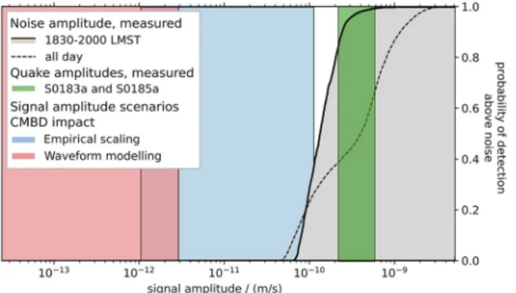
Figure 6. Detection probabilities for seismic signals of certain velocity amplitudes between 0.2 and 0.9 Hz. The solid black curve indicates the noise distribution considering the average signal amplitudes in only the early evening over 20 Sols during the same martian season in 2019, while the dashed black curve is for the whole period of 20 Sols. The shaded gray area indicates the regions in which signals are detectable. The blue and red bars mark the P wave amplitude estimates of the 75-kg CMBD impact, using the empirical scaling and wave propagation modeling estimates, respectively, described earlier in this paper. Vertical lines bounding the different sectors correspond to the upper and lower bounds derived from these methods, for the blue and red sectors, respectively (as an example,
vu and vl are the vertical edges of the red sector). For comparison, the
amplitudes of two previously detected tectonic marsquakes, S0183a and S0185a, located at comparable distances, are plotted in green.
Both of the consequences of the spacecraft's direction of travel being toward InSight are therefore to reduce the amplitude of any acoustic signal. As the signal is already well below the noise floor at the lander's loca-tion, neglecting these effects will not change the conclusions of this paper.
4.3.3. Low-Altitude Acoustic Sources
As discussed in Section 3.2, there are two potential low-altitude (i.e., within the tenuous tropospheric wave-guide) acoustic sources which occur as a result of the EDL sequence: the CMBD impact with the ground, and acoustic signal produced by the spacecraft once it is subsonic. The travel time to InSight for any such signal would be ∼4–5 h, though as discussed, no detection is expected and this section is included to illus-trate a methodology only.
Both of these will produce signals much weaker than the supersonic deceleration of the spacecraft, and in the case of the CMBD impacts quantitatively estimating the acoustic overpressure this will produce is chal-lenging due to the multi-phase and nonlinear nature of the problem.
For purely illustrative purposes, we consider an exemplar source of 1 Pa and 1 Hz frequency in the Mars 2020 landing region. This is a pressure perturbation ΔPP of ∼0.15%. This is substantially larger than most acoustic sources on Mars (Martire et al., 2020) and stronger and lower frequency than we expect either signal to be.
Even neglecting attenuation, the amplitude of this perturbation after propagating to the distance of InSight is no larger than 3 × 10⁻⁴ Pa (using a r−1 scaling) or 5 × 10⁻⁶ Pa (using a r−1.5 scaling). For comparison, both
values are far below the pressure noise floor of the APSS instrument (∼2 × 10⁻³ Pa in the 0.1–1 Hz range)
(Banfield et al., 2019; Martire et al., 2020).
4.3.4. Other Relevant Effects
For completeness, we also briefly detail other (lower-order) effects which may be relevant in applications of this methodology to other contexts.
The acoustic signal will be affected by surface topography and the temporal evolution of the atmosphere. If an acoustic signal was detected (which we do not expect to be the case here), more detailed consider of the nonlinear infrasound propagation in the near-source region should be conducted if the signal is to be clearly associated with an EDL event. It is possible that other kinds of atmospheric waves (e.g., internal gravity waves) may also be excited by an EDL event, though again this is not relevant to the case discussed in this paper.
Modeling of the elastodynamic signal in the solid ground may also include consideration of the source mechanism (as discussed in Section 3.3.2), and of three-dimensional heterogeneous effects including scat-tering and local geology.
5. Conclusions
We identified three possible types of seismoacoustic signals generated by the EDL sequence of the Perse-verance Rover: (1) the propagation of acoustic waves in the atmosphere formed by the decay of the Mach shock, (2) the seismoacoustic air-to-ground coupling of these waves inducing signals in the solid ground, and (3) the elastodynamic seismic waves propagating in the ground from the hypersonic impacts of the CMBDs.
(1) In the first case (atmospheric propagation), the stratification and wind structure in the atmosphere are such that the strongest signals produced will likely not be detectable at InSight, as they are reflected off the ground back up into the atmosphere. Signals produced in the lower 10 km of the atmosphere may be trapped and propagate for long distances; however, the spacecraft will be subsonic by this point and will not be emitting substantial amounts of acoustic energy into the atmosphere. The Mach shock