Accelerating dynamic programming

Accelerating Dynamic Programming

by

Oren Weimann

MASSACHUSETTS INSTTTUTE OF TECHNOLOGY

AUG 0 7

2009

LIBRARIES

Submitted to the Department of Electrical Engineering and Computer Science

in partial fulfillment of the requirements for the degree of

Doctor of Philosophy

at the

MASSACHUSETTS INSTITUTE OF TECHNOLOGY

June 2009

@

Massachusetts Institute of Technology 2009. All rights reserved.

Author ...

...

...

Department of Electrical Engineering and Compuer Science

February

5,

2009

Certified by

Erik D. Demaine

Associate Professor of Electrical Engineering and Computer Science

Thesis Supervisor

Accepted by ...

7,

_{Professor Terry P. Orlando}

Accelerating Dynamic Programming

by

Oren Weimann

Submitted to the Department of Electrical Engineering and Computer Science on February 5, 2009, in partial fulfillment of the

requirements for the degree of Doctor of Philosophy

Abstract

Dynamic Programming (DP) is a fundamental problem-solving technique that has been widely used for solving a broad range of search and optimization problems. While DP can be invoked when more specialized methods fail, this generality often incurs a cost in efficiency. We explore a unifying toolkit for speeding up DP, and algorithms that use DP as subroutines. Our methods and results can be summarized as follows.

- Acceleration via Compression. Compression is traditionally used to efficiently store data. We

use compression in order to identify repeats in the table that imply a redundant computation. Utilizing these repeats requires a new DP, and often different DPs for different compression schemes. We present the first provable speedup of the celebrated Viterbi algorithm (1967) that is used for the decoding and training of Hidden Markov Models (HMMs). Our speedup relies on the compression of the HMM's observable sequence.

- Totally Monotone Matrices. It is well known that a wide variety of DPs can be reduced to

the problem of finding row minima in totally monotone matrices. We introduce this scheme in the context of planar graph problems. In particular, we show that planar graph problems such as shortest paths, feasible flow, bipartite perfect matching, and replacement paths can be accelerated by DPs that exploit a total-monotonicity property of the shortest paths.

- Combining Compression and Total Monotonicity. We introduce a method for accelerating string

edit distance computation by combining compression and totally monotone matrices. In the heart of this method are algorithms for computing the edit distance between two straight-line programs. These enable us to exploits the compressibility of strings, even if each string is compressed using a different compression scheme.

- Partial Tables. In typical DP settings, a table is filled in its entirety, where each cell corresponds

to some subproblem. In some cases, by changing the DP, it is possible to compute asymptotically less cells of the table. We show that

E(n

3) subproblems are both necessary and sufficient for computing the similarity between two trees. This improves all known solutions and brings the idea of partial tables to its full extent.

- _{Fractional Subproblems. In some DPs, the solution to a subproblem is a data structure rather}

than a single value. The entire data structure of a subproblem is then processed and used to construct the data structure of larger subproblems. We suggest a method for reusing parts of a subproblem's data structure. In some cases, such fractional parts remain unchanged when constructing the data structure of larger subproblems. In these cases, it is possible to copy this part of the data structure to the larger subproblem using only a constant number of pointer changes. We show how this idea can be used for finding the optimal tree searching strategy in linear time. This is a generalization of the well known binary search technique from arrays to trees.

Thesis Supervisor: Erik D. Demaine

Acknowledgments

I am deeply indebted to my thesis advisor, Professor Erik Demaine. Erik's broad research

inter-ests and brilliant mind have made it possible to discuss and collaborate with him on practically

any problem of algorithmic nature. His open-minded view of research, and his support in my

research which was sometimes carried outside MIT, have provided me with the prefect research

environment. I feel privileged to have learned so much from Erik, especially on the subject of data structures.

I owe much gratitude to Professor Gad Landau. His guidance, kindness, and friendship

dur-ing my years in MIT and my years in Haifa have been indispensable. I am also thankful to the

MADALGO research center and the Caesarea Rothschild Institute for providing me with

addi-tional working environments and financial support.

This thesis is based primarily on the following publications: [I 1] from ICALP'07, [12 ] from

JCB, [ '] from SODA'08, [63] from Algorithmica, [52] from SODA'09, and ['5] from STACS'09. I would like to thank my collaborators in these publications. In particular, I am grateful for my

ongoing collaboration with Shay Mozes and Danny Hermelin, who make it possible for me to conduct research together with close friends.

Finally, I wish to express my love and gratitude to Gabriela, my parents, my grandparents, and

Contents

1 Introduction

13

1.1 Searching for DP Repeats ... ... 14

1.2 Totally Monotone Matrices ... ... . . . ... . 16

1.3 Partial Tables and Fractional Subproblems . ... . . . . . 18

2 Acceleration via Compression 21 2.1 Decoding and Training Hidden Markov Models . ... 22

2.1.1 The Viterbi Algorithm ... . . . ... .. 23

2.1.2 The Forward-Backward Algorithms ... ... . 25

2.2 Exploiting Repeated Substrings . ... ... 25

2.3 Five Different Implementations of the General Framework . ... 27

2.3.1 Acceleration via the Four Russians Method . ... 27

2.3.2 Acceleration via Run-length Encoding . ... . 28

2.3.3 Acceleration via LZ78 Parsing . ... ... 29

2.3.4 Acceleration via Straight-Line Programs . ... 32

2.3.5 Acceleration via Byte-Pair Encoding ... .. 34

2.4 Optimal state-path recovery . ... . ... . 35

2.5 The Training Problem ... ... 36

2.5.1 Viterbi training ... .. ... 37

2.5.2 Baum-Welch training ... ... ... 37

2.6 Parallelization ... .... . ... 40

3 Totally Monotone Matrices and Monge Matrices 43

3.1 Preliminaries . . . . ... . 46

3.1. I Monotonicity, Monge and Matrix Searching. . ... . . 46

3.1.2 Jordan Separators for Embedded Planar Graphs. . ... 48

3.2 A Bellman-Ford Variant for Planar Graphs ... ... 49

3.3 The Replacement-Paths Problem in Planar Graphs . ... 54

4 Combining Compression and Total-Monotonicity 59 4. I1 Accelerating String Edit Distance Computation ... . . . . . . . ..... 60

4. 1. 1 Straight-line programs . ... . . ... . 61

4.1.2 Our results . . . ... ... 62

4.1.3 Related Work ... ... . . 63

4.2 The DIST Table and Total-Monotonicity . ... . 64

4.3 Acceleration via Straight-Line Programs ... ... ... . . 66

4.3.1 Constructing an ry-partition . ... 69

4.4 Improvement for Rational Scoring Functions ... . . . . . . . . . . . 71

4.5 Four-Russian Interpretation .... . . . . . . . ... 72

5 Partial Tables 75 5.1 Tree Edit Distance . . . . ... ... . 76

5.1.1 Shasha and Zhang's Algorithm ... ... . . 79

5.1.2 Klein's Algorithm . . . ... ... ... . 80

5.1.3 The Decomposition Strategy Framework . ... 81

5.2 Our Tree Edit Distance Algorithm . ... . . . . . 83

5.3 A Space-Efficient DP formulation ... .. ... . 88

5.4 A Tight Lower Bound for Decomposition Algorithms . ... 95

5.5 Tree Edit Distance for RNA Comparison ... . .. 99

5.5.1 RNA Alignment . ... .. . . . 101

5.5.2 Affine Gap Penalties . . . . . . . . ... . 102

6 Fractional Subproblems

105

6.1 Finding an Optimal Tree Searching Strategy in Linear Time . ... 106

6.2 Machinery for Solving Tree Searching Problems . ... ... .. . . 109

6.3 Computing a Minimizing Extension ... . . . .. . ... . . 111

6.3.1 Algorithm Description. ... ... . . . 111

6.4 Linear Time Solution via Fractional Subproblems . ... 118

6.5 From a Strategy Function to a Decision Tree in Linear Time . .... . ... . 125

An HMM and the optimal path of hidden states . ... The Viterbi algorithm ... ...

The Fibonacci straight-line program (SLP) . ... A "good" substring in the Baum-Welch training . ...

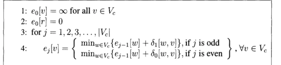
3-1 The Bellman-Ford algorithm . ...

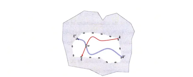
3-2 Decomposing a planar graph using a Jordan curve . . . . 3-3 Decomposing a shortest path into external and internal paths . 3-4 Pseudocode for the single-source boundary distances . . . . . 3-5 Crossing paths between boundary nodes . . . .... 3-6 Two crossing LL replacement paths . . . .... 3-7 Two crossing LR replacement paths . . . .. 3-8 The upper triangular fragment of the matrix lend .. . . .

4-1 A subgraph of a Levenshtein distance DP graph . . . . 4-2 An 'ry-partition...

4-3 A closer look on the parse tree of an SLP A. . . . . 5-1 The three editing operations on a tree . . . . . ..

5-2 A tree F with its heavy path and TopLight(F) vertices . . . .

5-3 The intermediate left subforest enumeration . . . . 5-4 The indexing of subforests G, ...

5-5 The two trees used to prove an Q( r 2_{o) lower bound . . . . .}

. . . . . . . 49 . . . . . 50 . . . . . 50 . . . . . 51 . . . . . 53 . . . . . 55 . . . . . . 55 . . . . . . . 57 . . . . . 64 ... . 67 . . . . . . 70 . . . . . 77 . . . . . 84 . . . . . 90 . . . . . 91 . . . . . 96

List of Figures

2-1 2-2 2-3 2-4 . . . 23 . . . 24 . . . 32 . . . 39

5-6 The two trees used to prove an 2 _{lg -}IO((_{) lower bound. . . . .}

97

5-7 Three different ways of viewing an RNA sequence . ... 100

5-8 Two example alignments for a pair of RNA sequences. . ... 102

6-1 An optimal strategy for searching a tree ... .. .. . .... .. 110

Chapter 1

Introduction

Dynamic Programming (DP) is a powerful problem-solving paradigm in which a problem is solved

by breaking it down into smaller subproblems. These subproblems are then tackled one by one,

so that the answers to small problems are used to solve the larger ones. The simplicity of the DP paradigm, as well as its broad applicability have made it a fundamental technique for solving

various search and optimization problems.

The word "programming" in "dynamic programming" has actually very little to do with

com-puter programming and writing code. The term was first coined by Richard Bellman in the 1950s,

back when programming meant planning, and dynamic programming meant to optimally plan a

solution process. Indeed, the challenge of devising a good solution process is in deciding what are

the subproblems, and in what order they should be computed. Apart from the obvious requirement

that an optimal solution to a problem can be obtained by optimal solutions to its subproblems, an

efficient DP is one that induces only a "small" number of distinct subproblems. Each subproblem

is then reused again and again for solving multiple larger problems.

This idea of reusing subproblems is the main advantage of the DP paradigm over recursion.

Recursion is suited for design techniques such as divide-and-conquer, where a problem is reduced

to subproblems that are substantially smaller, say half the size. In contrast, in a typical DP setting,

a problem is reduced to subproblems that are only slightly smaller (e.g., smaller by only a constant factor). However, it is often convenient to write out a top-down recursive formula and then use

it to describe the corresponding bottom-up DP solution. In many cases, this transformation is not immediate since in the final DP we can often achieve a space complexity that is asymptotically

smaller than the total number of subproblems. This is enhanced by the fact that we only need to store the answer of a subproblem until the larger subproblems depending on it have been solved.

The simplicity of the DP paradigm is what makes it appealing, both as a full problem solving method as well as a subroutine solver in more complicated algorithmic solutions. However, while DP is useful when more specialized methods fail, this generality often incurs a cost in efficiency. In this thesis, we explore a toolkit for speeding up straightforward DPs, and algorithms that use DPs as subroutines.

To illustrate some DP ideas, consider the string edit distance problem. This problem asks to compute the minimum number of character deletions, insertions, and replacements required to transform one string A = ala2 ... an into another string B = bib2... bn. Let E(i,

j)

denote the edit distance between ala2 .. ai and b1b2 ... bj. Our goal is then to compute E(n, m), and we can

achieve this by using the following DP.

E(i,j) =min{E(i,j - 1)+1, E(i-1,j) + 1, E(i - 1,j- 1)+diff(i,j)}

where diff(i,j) = 0 if ai = by, and 1 otherwise. This standard textbook DP induces O(nm) subproblems - one subproblem for each pair of prefixes of A and B. Since every subproblem requires the answers to three smaller subproblems, the time complexity is O(nm) and the bottom-up DP can construct the table E row by row. Notice that at any stage during the computation, we only need to store the values of two consecutive rows, so this is a good example of a situation where the space complexity is smaller than the time complexity (the number of subproblems).

1.1

Searching for DP Repeats

As we already mentioned, a good DP solution is one that makes the most out of subproblem repeats. Indeed, if we look at a subproblem E(i,

j),

it is used for solving the larger subproblem

repeats to their full extent? What if the string A = A'A' (i.e., A is the concatenation of two equal

strings of length n/2), and B = B'B'. The DP computation will then behave "similarly" on E(i, j)

and on E(i + n/2, j + m/2) for every i = 1,..., n/2 and j = 1,..., m/2. In order for repeats

in the strings to actually induce repeated subproblems we would have to modify the DP so that

subproblems correspond to substrings rather than to prefixes of A and B.

The first paper to do this and break the quadratic time upper bound of the edit distance

com-putation was the seminal paper of Masek and Paterson [72]. This was achieved by applying the

so called "Four-Russians technique" - a method based on a paper by Arlazarov, Dinic, Kronrod, and Faradzev [ 10] for boolean matrix multiplication. The general idea is to first pre-compute the

subproblems that correspond to all possible substrings (blocks) of logarithmic size, and then

mod-ify the edit distance DP so instead of advancing character by character it advances block by block.

This gives a logarithmic speedup over the above O(nm) solution.

The Masek and Paterson speedup is based on the fact that in strings over constant-sized

al-phabets, small enough substrings are guaranteed to repeat. But what about utilizing repeats of longer substrings? It turns out that we can use text compression to both find and utilize

re-peats. The approach of using compression to identify DP repeats, denoted "acceleration via

com-pression", has been successfully applied to many classical string problems such as exact string

matching [5, 4), , '], ], approximate pattern matching [i, .4, 49, 82], and string edit

dis-tance [ , , 2, ), , 2]. It is often the case that utilizing these repeats requires an entirely new (and more complicated) DP.

It is important to note, that all known improvements on the O(nm) upper bound of the edit

distance computation, apply acceleration via compression. In addition, apart from the naive

com-pression of the Four-Russians technique, Run Length Encoding, and the LZW-LZ78 comcom-pression,

we do not know how to compute the edit distance efficiently under other compression schemes.

Our string edit distance result. We introduce a general compression-based edit distance al-gorithm that can exploit the compressibility of two strings under any compression scheme, even

if each string is compressed with a different compression. This is achieved by using Straight-line programs (a notion borrowed from the world of formal languages), together with an efficient

algorithm for finding row minima in totally monotone matrices. We describe the use of totally monotone matrices for accelerating DPs in Section 1.2.

Our HMM result. Hidden Markov Models (HMMs) are an extremely useful way of modeling

processes in diverse areas such as error-correction in communication links

[ ],

speech recogni-tion [ i

1],

optical character recognition [ i], computational linguistics [ ], and bioinformatics [

1

]. The two most important computational problems involving HMMs are decoding and training. The problem of decoding an HMM asks to find the most probable sequence of hidden states to have generated some observable sequence, and the training problem asks to estimate the model given only the number of hidden states and an observable sequence.

In Chapter 2, we apply acceleration via compression to the DP algorithms used for decoding and training HMMs. We discuss the application of our method to Viterbi's decoding and train-ing algorithms [ ], as well as to the forward-backward and Baum-Welch [ ] algorithms. We obtain the first provable speedup of the celebrated Viterbi algorithm [ ]. Compared to Viterbi's algorithm, we achieve speedups of O(log n) using the Four-Russians method, Q ( ' ) using run-length encoding, t(- -) using Lempel-Ziv parsing, Q( ) using straight-line programs, and nQ(r) using byte-pair encoding, where k is the number of hidden states, n is the length of the observed sequence and r is its compression ratio (under each compression scheme).

1.2 Totally Monotone Matrices

One of the best known DP speedup techniques is the seminal algorithm of Aggarwal, Klawe, Moran, Shor, and Wilber [,] nicknamed SMAWK in the literature. This is a general speedup technique that can be invoked when the DP satisfies additional conditions of convexity or concavity that can be described by a totally monotone matrix. An n x m matrix M = (Mi) is totally

monotone if for every i, i', j, j' such that i < i', j <

j',

and Mi < Mij,, we have that M,'j < M,j,. Aggarwal et al. showed that a wide variety of problems in computational geometry can be reduced to the problem of finding row minima in totally monotone matrices. The SMAWK algorithm finds all row minima optimally in O(n + m) time. Since then, many papers on applications which lead

to totally monotone matrices have been published (see

[20

] for a survey).

Our planar shortest paths result. In Chapter 3, we use totally monotone matrices in the context

of planar graph problems. We take advantage of the fact that shortest paths in planar graphs exhibit

a property similar to total-monotonicity. Namely, they can be described by an upper-triangular

fragment of a totally monotone matrix. Our first result is an O(na(n)) time' DP for preforming a

variant of the Bellman-Ford shortest paths algorithm on the vertices of the planar separator. This

DP serves as a subroutine in all single-source shortest paths algorithms for directed planar graphs

with negative edge lengths. The previous best DP for this subroutine is that of Fakcharoenphol and

Rao [3 5] and requires O(n log2 n) time.

Fakcharoenphol and Rao used this subroutine (and much more) to obtain an O(n log3

n)-time and O(n log n)-space solution for the single-source shortest paths problem in directed

pla-nar graphs with negative lengths. In [52], we used our new DP to improve this to O(n log2 _n) time and O(n) space. This result is important not only for shortest paths, but also for solving

bipartite perfect matching, feasible flow, and feasible circulation which are all equivalent in planar

graphs to single-source shortest paths with negative lengths. Apart from the DP, we needed other

non-DP ideas that are beyond the scope of this thesis. We therefore focus here only on the said Bellman-Ford variant.

Our planar replacement paths result. Our second result involving total-monotonicity in planar

graphs concerns the replacement-paths problem. In this problem, we are given a directed graph

with non-negative edge lengths and two nodes s and t, and we are required to compute, for every

edge e in the shortest path between s and t, the length of an s-to-t shortest path that avoids e. By

exploiting total-monotonicity, we show how to improve the previous best O(n log3 n)-time solution

of Emek et al. [3.4] for the replacement path problem in planar graphs to O(n log2 n).

Finally, as we already mentioned, by combining acceleration via compression, and the totally

monotone properties of the sting edit distance DP, we show in Chapter 4 how to accelerate the string edit distance computation.

1.3

Partial Tables and Fractional Subproblems

The main advantage of (top-down) recursion over (bottom-up) DP is that while DP usually solves every subproblem that could conceivably be needed, recursion only solves the ones that are actually used. We refer to these as relevant subproblems. To see this, consider the Longest Common

Subsequence (LCS) problem that is very similar to string edit distance. The LCS of two strings

A = aja2 . .. a and B = bb2 ... bm is the longest string that can be obtained from both A and

B by deleting characters. As in the edit distance case, we let L(i, j) denote the length of the LCS

between ala2 .. ai and b1b2. bj, and we compute L(n, m) using the following DP.

(ij) L(i-1,j-1) +1 ,if a = bj

max{L(i,j - 1) + 1,L(i - 1,j) + 1} ,otherwise

Like the edit distance DP, the LCS DP will solve O(nm) subproblems, one for each pair of pre-fixes of A and B. However, consider a simple scenario in which A = B. In this case, a recursive

implementation will only compute O(n) distinct (relevant) subproblems (one for each pair of pre-fixes of A and B of the same length), while DP will still require Q(n 2_{). To avoid computing the} same subproblem again and again, one could use memoization - a recursive implementation that remembers its previous invocations (using a hash table for example) and thereby avoids repeating them.

There are two important things to observe from the above discussion. First, that in the worst case (for general strings A and B), both the recursion (or memoization) and the DP compute Q(n2)

distinct subproblems. Second, the memoization solution does not allow reducing the space com-plexity. That is, the space complexity using memoization is equal to the number of subproblems, while in DP it can be reduced to O(n) even when the number of relevant subproblems is Q (n2_).

Surprisingly, in some problems (unfortunately not in LCS), these two obstacles can be over-come. For such problems, it is possible to slightly change their original DP, so that it will fill only a partial portion of the DP table (i.e., only the subset of relevant subproblems). It can then be shown that even in the worst case, this partial portion is asymptotically smaller than the entire table. Furthermore, the space complexity can be reduced to be even smaller than the size of this

partial portion.

The main advantage of the partial table idea is that a slight change in the DP can make a big change in the number of subproblems that it computes. While the analysis can be complicated, the actual DP remains simple to describe and implement. This will be the topic of Chapter 5.

Our tree edit distance result. In Chapter 5, we will apply the above idea to the problem of tree edit distance. This problem occurs in various areas where the similarity between trees is sought.

These include structured text databases like XML, computer vision, compiler optimization, natural language processing, and computational biology [1 5, .2 , 5 4, ', ].

The well known DP solution of Shasha and Zhang [88] to the tree edit distance problem in-volves filling an O(n4)-sized table. Klein [513], showed that a small change to this DP induces only O(n3 log n) relevant subproblems. We show that 8(n3) subproblems are both necessary and sufficient for computing the tree edit distance DP. This brings the idea of filling only a partial DP table to its full extent. We further show how to reduce the space complexity to O(n2_).

After describing the idea of partial tables, the final chapter of this thesis deals with partial subproblems. Notice that in both DPs for edit distance and LCS that we have seen so far, the answer to a subproblem is a single value. In some DPs however, the solution to a subproblem is an entire data structure rather than only a value. In these cases, the DP solution processes the entire data structure computed for a certain subproblem in order to construct the data structure of larger subproblems. In Chapter 6, we discuss processing only parts of a subproblem's data structure. We show that in some cases, a part of a subproblem's data structure remains unchanged when computing the data structure of larger subproblems. In these cases, it is possible to copy this part of the data structure to the larger subproblem using only a constant number of pointer changes.

Our tree searching result. We show how this idea can be used for the problem of finding an

optimal tree searching strategy. This problem is an extension of the binary search technique from sorted arrays to trees, with applications in file system synchronization and software testing [

~4,

S07,

83]. As in the sorted array case, the goal is to minimize the number of queries required to find a target element in the worst case. However, while the optimal strategy for searching an array

is straightforward (always query the middle element), the optimal strategy for searching a tree is dependent on the tree's structure and is harder to compute. We give an O(n) time DP solution that uses the idea of fractional subproblems and improves the previous best O(n3_{)-time algorithm of} Onak and Parys [x ].

Chapter 2

Acceleration via Compression

The main idea of DP is that subproblems that are encountered many times during the computation

are solved once, and then used multiple times. In this chapter, we take this idea another step

forward by considering entire regions of the DP table that appear more than once. This is achieved

by first changing the DP in a way that regional repeats are guaranteed to occur, and then using text

compression as a tool to find them.

The traditional aim of text compression is the efficient use of resources such as storage and bandwidth. The approach of using compression in DP to identify repeats, denoted "accelera-tion via compression", has been successfully applied to many classical string problems. Vari-ous compression schemes, such as Lempel-Ziv [ i04, 1ti0], Huffman coding, Byte-Pair

Encod-ing [90], Run-Length Encoding, and Straight-Line Programs were employed to accelerate exact

string matching [5, , '~l , 70, Q 1], approximate pattern matching [4, 48, 4), 8i], and string edit

distance [-, ", 1", 29, 69].

The acceleration via compression technique is designed for DPs that take strings as inputs.

By compressing these input strings, it is possible to identify substring repeats that possibly imply

regional repeats in the DP itself. In this chapter, we investigate this technique on a problem that is

not considered a typical string problem as its input does not consist only of strings. We present a method to speed up the DPs used for solving Hidden Markov Model (HMM) decoding and training

We discuss the application of our method to Viterbi's decoding and training algorithms [

],

as well as to the forward-backward and Baum-Welch [ ] algorithms.

In Section 2.1 we describe HMMs, and give a unified presentation of the HMM DPs. Then, in Section 2.2 we show how these DPs can be improved by identifying repeated substrings. Five different implementations of this general idea are presented in Section 2.3: Initially, we show how to exploit repetitions of all sufficiently small substrings (the Four-Russians method). Then, we describe four algorithms based alternatively on Run-Length Encoding (RLE), Lempel-Ziv (LZ78), Straight-Line Programs (SLP), and Byte-Pair Encoding (BPE). Compared to Viterbi's algorithm, we achieve speedups of O(log n) using the Four Russians method, Q( ' ) using RLE, Q( 1-) using LZ78,

Q(-)

using SLP, and Q(r) using BPE, where k is the number of hidden states, n is the length of the observed sequence and r is its compression ratio (under each compression scheme). We discuss the recovery of the optimal state-path in Section 2.4, and the adaptation of our algorithms to the training problem in Section 2.5. Finally, in Section 2.6 we describe a parallel implementation of our algorithms.

2.1

Decoding and Training Hidden Markov Models

Over the last few decades HMMs proved to be an extremely useful framework for modeling processes in diverse areas such as error-correction in communication links [ ], speech

recogni-tion [ ], optical character recognirecogni-tion [ ], computarecogni-tional linguistics [ ], and bioinformatics [ ].

Definition 2.1 (Hidden Markov Model) Let E denote a finite alphabet and let X E E', X = xi, 2, ... , xn be a sequence of observed letters. A Markov model is a set of k states, along with emission probabilities ek((a) - _{the probability to observe a E E given that the state is k, and} transition probabilities Pj - _{the probability to make a transition to state i from state}

_j.

The core HMM-based applications fall in the domain of classification methods and are tech-nically divided into two stages: a training stage and a decoding stage. During the training stage, the emission and transition probabilities of an HMM are estimated, based on an input set of ob-served sequences. This stage is usually executed once as a preprocessing stage and the generated

("trained") models are stored in a database. Then, a decoding stage is run, again

and again, in

order to classify input sequences. The objective of this stage is to find the most probable sequence

of states to have generated each input sequence given each model, as illustrated in Fig. 2-1.

IX I

I

I

X1 X2 X3 ... Xn

Figure 2-1: The HMM on the observed sequence X = xl, x2,.. .,

xn

and states 1, 2,..., k. The

highlighted path is a possible path of states that generate the observed sequence. VA finds the path

with highest probability.

Obviously, the training problem is more difficult to solve than the decoding problem. However,

the techniques used for decoding serve as basic ingredients in solving the training problem. The

Viterbi algorithm (VA)

[99]

is the best known tool for solving the decoding problem. Following its

invention in 1967, several other algorithms have been devised for the decoding and training

prob-lems, such as the forward-backward and Baum-Welch [t 3] algorithms. These algorithms are all

based on DP and their running times depend linearly on the length of the observed sequence. The

challenge of speeding up VA by utilizing HMM topology was posed in 1997 by Buchsbaum and

Giancarlo [ 18] as a major open problem. We address this open problem by using text compression

and present the first provable speedup of these algorithms.

2.1.1 The Viterbi Algorithm

The Viterbi algorithm (VA) finds the most probable sequence of hidden states given the model and

the observed sequence, i.e., the sequence of states sl, S2,... , Sn which maximize

e s(xi) Ps',

l1

(2.1)

The DP of VA calculates a vector vt [i] which is the probability of the most probable sequence of states emitting xl,..., _{xt and ending with the state i at time t. vo is usually taken to be the vector}

of uniform probabilities (i.e., voi] _{= 1). Vt+l is calculated from vt according to}

t+l [i] = ei(xt+l) -max{Pi,j - vt[j]} _(2.2)

Definition 2.2 (Viterbi Step) We call the computation of vt+l from vt a Viterbi step. Clearly, each Viterbi step requires O(k2

) time. Therefore, the total runtime required to compute the

vector v, is O(nk2

). The probability of the most likely sequence of states is the maximal element

in v,. The actual sequence of states can then be reconstructed in linear time.

4

6

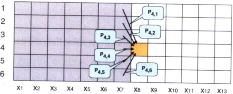
. . 4,

Xi X2 X3 X4 X5 X6 X7 X8 X9 X10 X11 X12 X13

Figure 2-2: The VA dynamic programming table on sequence X = £1, x2, .. ,x13 and states 1, 2, 3, 4, 5, 6. The marked cell corresponds to v8

[4]

= e4(x8)

-

max{P4,1 .7 1], P4,2.v7 [2],..., P4,6

V7[6]}.

It is useful for our purposes to rewrite VA in a slightly different way. Let M' be a k x k matrix with elements MZ,.- = ei(a) - P,j. We can now express v, as:

v, = Mxn 0 Mn - ( ) ... M2 O Mxl1 0 Vo (2.3)

where (A 0 B)i,j - maXk{Ai,k ' Bk,j _{is the so called max-times matrix multiplication. Similar}

notation was already considered in the past. In [ 17], for example, writing VA as a linear vector re-cursion allowed the authors to employ parallel processing and pipelining techniques in the context of VLSI and systolic arrays.

VA computes v, using (2.3) from right to left in O(nk

2

_{) time. Notice that if (2.3) is}

evalu-ated from left to right the computation would take O(nk

3

_{) time (matrix-vector multiplication vs.}

matrix-matrix multiplication). Throughout, we assume that the max-times matrix-matrix

multipli-cations are done naively in O(k

3

). Faster methods for max-times matrix multiplication [22, 2"]

and standard matrix multiplication [2,

j!4]

can be used to reduce the

k3

term. However, for small

values of k this is not profitable.

2.1.2

The Forward-Backward Algorithms

The forward-backward algorithms are closely related to VA and are based on very similar DP.

In contrast to VA, these algorithms apply standard matrix multiplication instead of max-times

multiplication. The forward algorithm calculates ft[i], the probability to observe the sequence

x1, X2,..., Xt requiring that st = i as follows:

ft = Mx t .MX -1 . MX2

.Mx

.

fo

(2.4) The backward algorithm calculates bt [i], the probability to observe the sequence Xt+l, t+2, .. , Xn given that st = i as follows:

bt = bn - M xn .Mx n - 1 ... M t+2

.Mx t+1 (2.5)

Another algorithm which is used in the training stage and employs the forward-backward algorithm

as a subroutine, is the Baum-Welch algorithm, to be further discussed in Section 2.5.

2.2

Exploiting Repeated Substrings

Consider a substring W = w, 1 2, ... , we of X, and define

M(W) = Mn 0 MWI- 1 0( _{.0 MW} 2 _{0 M}I _'

Intuitively, Mi, (W) is the probability of the most likely path starting with state

j,

making a transi-tion into some other state, emitting wl, then making a transitransi-tion into yet another state and emitting

w2 and so on until making a final transition into state i and emitting w.

In the core of our method stands the following observation, which is immediate from the

asso-ciative nature of matrix multiplication.

Observation 2.3 We may replace any occurrence of Mwl

0

MZ " -1 - ... M" in eq. (2.3) with

M(W).

The application of observation 1 to the computation of equation (2.3) saves f - 1 Viterbi steps each

time W appears in X, but incurs the additional cost of computing M(W) once.

An intuitive exercise. Let A denote the number of times a given word W appears, in

non-overlapping occurrences, in the input string X. Suppose we naively compute M(W) using (IWI

-1) max-times matrix multiplications, and then apply observation 1 to all occurrences of W before

running VA. We gain some speedup in doing so if

(IWI-

1)k3

₊

_Ak2 _<

_A1W;

_k

2

A > k (2.7)

Hence, if there are at least k non-overlapping occurrences of W in the input sequence, then it is

worthwhile to naively precompute M(W), regardless of its size WI.

Definition 2.4 (Good Substring) We call a substring W good if we decide to compute M(W).

We can now give a general four-step framework of our method:

(I) Dictionary Selection: choose the set D = {Wi} of good substrings.

(II) Encoding: precompute the matrices M(Wi) for every Wi E D.

(III) Parsing: partition the input sequence X into consecutive good substrings so that X =

W, Wi,2 ... Wi ,, and let X' denote the compressed representation of this parsing of X,

(IV) Propagation: run VA on X', using the matrices M(W).

The above framework introduces the challenge of how to select the set of good substrings (step

I) and how to efficiently compute their matrices (step II). In the next section we show how the

RLE, LZ78, SLP and BPE compression schemes can be applied to address this challenge, and how

the above framework can be utilized to exploit repetitions of all sufficiently small substrings (this

is similar to the Four Russians method). In practice, the choice of the appropriate compression

scheme should be made according to the nature of the observed sequences. For example, genomic

sequences tend to compress well with BPE

[I2]

and binary images in facsimile or in optical

char-acter recognition are well compressed by RLE

[

, 8, '), 19, (,,

7,].

LZ78 guarantees asymptotic

compression for any sequence and is useful for applications in computational biology, where k is

smaller than log n [ i 7, 2 7, 3].

Another challenge is how to parse the sequence X (step III) in order to maximize acceleration.

We show that, surprisingly, this optimal parsing may differ from the initial parsing induced by

the selected compression scheme. To our knowledge, this feature was not applied by previous

"acceleration by compression" algorithms.

We focus on computing path probabilities rather than the paths themselves. The actual paths

can be reconstructed in linear time as described in Section

2.4.

2.3 Five Different Implementations of the General Framework

In this section, we present five different ways of implementing the general framework, based

alter-natively on the Four Russians method, and the RLE, LZ78, SLP, and BPE compression schemes.

We show how each compression scheme can be used for both selecting the set of good substrings

(step I) and for efficiently computing their matrices (step II).

2.3.1 Acceleration via the Four Russians Method

The most naive approach is probably using all possible substrings of sufficiently small length £ as

good ones. This approach is quite similar to the Four Russians method

[

I

],

and leads to a

O

(log n)

asymptotic speedup. The four-step framework described in Section 2.2 is applied as follows.

(I) Dictionary Selection: all possible strings of length f over alphabet IE are good substrings.

(II) Encoding: For i = 2...

£,

compute M(W) for all strings W with length i by computing

M(W') 0 M(a), where W = W'u for some previously computed string W' of length

i - 1 and some letter a E .

(III) Parsing: X' is constructed by partitioning the input X into blocks of length f.

(IV) Propagation: run VA on X', using the matrices M(Wi) as described in Section 2.2.

Time and Space Complexity. The encoding step takes 0(2|E|'k3) time as we compute 0(2 EI')

matrices and each matrix is computed in O(k3) time by a single max-times multiplication. The

propagation step takes 0("2 ) time resulting in an overall running time of 0(2 EZlk

3 _{+ "k}2

) Choosing f ₂ logj (n), the running time is O(2x/ k3 + 2nk2). _{). This yields a speedup of}This yields a speedup of

S(log n) compared to VA, assuming that k < _{lOgl p(n)"}.In fact, the optimal length is approximately

= log n-log log n-log _log JE k-1, since then the preprocessing and the propagation times are roughly equal. This yields a E({) =

E(log

n) speedup, provided that f > 2, or equivalently that k < 2njlogn. Note that for large k the speedup can be further improved using fast matrix multiplication [, ,

2.3.2

Acceleration via Run-length Encoding

In this section we obtain an Q( o' ) speedup for decoding an observed sequence with run-length

compression ratio r. A string S is run-length encoded if it is described as an ordered sequence of

pairs (a, i), often denoted ai. Each pair corresponds to a run in S, consisting of i consecutive oc-currences of the character a. For example, the string aaabbcccccc is encoded as a3b2c6. Run-length encoding serves as a popular image compression technique, since many classes of images (e.g., bi-nary images in facsimile transmission or for use in optical character recognition) typically contain large patches of identically-valued pixels. The four-step framework described in Section 2.2 is

(I) Dictionary Selection: for every c E E and every i = 1,2,..., log n we choose o2_{' as a}

good substring.

(II) Encoding: since M(o-2i) M(a2 i-1_{) 0 M(o-2i-1), we can compute the matrices using}

repeated squaring.

(III) Parsing: Let W₁ W2 .. W, be the RLE of X, where each Wi is a run of some 0 E E. X'

is obtained by further parsing each Wi into at most log I Wi

I

good substrings of the form -2

.

(IV) Propagation: run VA on X', as described in Section 2.2.

Time and Space Complexity. The offline preprocessing stage consists of steps I and II. The time

complexity of step II is O( E Ik3 log n) by applying max-times repeated squaring in O(k3) time per

multiplication. The space complexity is O(IjEk 2 log n). This work is done offline once, during

the training stage, in advance for all sequences to come. Furthermore, for typical applications, the

O( EIk3 log n) term is much smaller than the O(nk2) term of VA.

Steps III and IV both apply one operation per occurrence of a good substring in X': step III

computes, in constant time, the index of the next parsing-comma, and step IV applies a single

Viterbi step in k2 time. Since

IX'l

= E 1 log Wi, the complexity is

wX'log

i

l og(II

Wl. W2.w,)1

...

--k

2

_{1W' = k}

2

_log(|Wi

_W)

< k

22Og)

(n/n'

)

0(n'k

2

_{lOg ).}

i=1

Thus, the speedup compared to the O(nk2) time of VA is Q( -) = "(-r).

2.3.3 Acceleration via LZ78 Parsing

In this section we obtain an Q( o) speedup for decoding, and a constant speedup in the case

where k > log n. We show how to use the LZ78 [1

i]

parsing to find good substrings and how to use the incremental nature of the LZ78 parse to compute M(W) for a good substring W in O(k3)

LZ78 parses the string X into substrings ( words) in a single pass over X. Each

LZ78-word is composed of the longest LZ78-LZ78-word previously seen plus a single letter. More formally,

LZ78 begins with an empty dictionary and parses according to the following rule: when parsing

location i, look for the longest LZ78-word W starting at position i which already appears in the

dictionary. Read one more letter ar and insert Wa into the dictionary. Continue parsing from

position i + W| + 1. For example, the string "AACGACG" is parsed into four words: A, AC, G,

ACG. Asymptotically, LZ78 parses a string of length n into O(hn/ log n) words [ ], where 0 <

h < 1 is the entropy of the string. The LZ78 parse is performed in linear time by maintaining the

dictionary in a trie. Each node in the trie corresponds to an LZ78-word. The four-step framework

described in Section 2.2 is applied as follows.

(I) Dictionary Selection: the good substrings are all the LZ78-words in the LZ78-parse of X.

(II) Encoding: construct the matrices incrementally, according to their order in the LZ78-trie,

M(Wr) = M(W) 0 M".

(III) Parsing: X' is the LZ78-parsing of X.

(IV) Propagation: run VA on X', as described in Section 2.2.

Time and Space Complexity. Steps I and III were already conducted offline during the

pre-processing compression of the input sequences (in any case LZ78 parsing is linear). In step II,

computing M(Wo) = M(W) 0 M', takes O(k3) time since M(W) was already computed for the good substring W. Since there are O(n/ log n) LZ78-words, calculating the matrices M(W) for

all Ws takes O(k3n/ log n). Running VA on X' (step IV) takes just O(k2n/ log n) time. Therefore,

the overall runtime is dominated by O(k3n/ log n). The space complexity is O(k2n/ log n).

The above algorithm is useful in many applications, where k < log n. However, in those

applications where k > log n such an algorithm may actually slow down VA. We next show an

adaptive variant that is guaranteed to speed up VA, regardless of the values of n and k. This

graceful degradation retains the asymptotic ( (1) acceleration when k < log n.

An improved algorithm with LZ78 Parsing

Recall that given M(W) for a good substring W, it takes k3 time to calculate M(Wo). This calculation saves k2 operations each time Wa occurs in X in comparison to the situation where only M(W) is computed. Therefore, in step I we should include in D, as good substrings, only

words that appear as a prefix of at least k LZ78-words. Finding these words can be done in a

single traversal of the trie. The following observation is immediate from the prefix monotonicity

of occurrence tries.

Observation 2.5 Words that appear as a prefix of at least k LZ78-words are represented by trie nodes whose subtrees contain at least k nodes.

In the previous case it was straightforward to transform X into X', since each phrase p in the

parsed sequence corresponded to a good substring. Now, however, X does not divide into just

good substrings and it is unclear what is the optimal way to construct X' (in step III). Our approach

for constructing X' is to first parse X into all LZ78-words and then apply the following greedy

parsing to each LZ78-word W: using the trie, find the longest good substring w' E D that is a

prefix of W, place a parsing comma immediately after w' and repeat the process for the remainder

of W.

Time and Space Complexity. The improved algorithm utilizes substrings that guarantee

accel-eration (with respect to VA) so it is therefore faster than VA even when k = Q(log n). In addition,

in spite of the fact that this algorithm re-parses the original LZ78 partition, the algorithm still

guarantees an

Q(

19) speedup over VA as shown by the following lemma.

Lemma 2.6 The running time of the above algorithm is bounded by O(k3n/log n).

Proof. The running time of step II is at most O(k3n/ log n). This is because the size of the entire

LZ78-trie is O(n/ log n) and we construct the matrices, in O(k3) time each, for just a subset of

the trie nodes. The running time of step IV depends on the number of new phrases (commas) that result from the re-parsing of each LZ78-word W. We next prove that this number is at most k for each word.

Consider the first iteration of the greedy procedure on some LZ78-word W. Let w' be the

longest prefix of W that is represented by a trie node with at least k descendants. Assume, contrary to fact, that I WI -

Iw'

> k. This means that w", the child of w', satisfies IWI -

Iw"

> k, in

contradiction to the definition of w'. We have established that (W - Iw') < k and therefore the number of re-parsed words is bounded by k + 1. The propagation step IV thus takes O(k3) time

for each one of the O(n/ log n) LZ78-words. So the total time complexity remains O(k3n/ log n).

Based on Lemma 2.6, and assuming that steps I and III are pre-computed offline, the running

time of the above algorithm is O(nk2/e) where e = Q(max(1, 12)). The space complexity is

O(k2n/logn).

2.3.4 Acceleration via Straight-Line Programs

In this subsection we show that if an input sequence has a grammar representation with

compres-sion ratio r, then HMM decoding can be accelerated by a factor of Q(L).

Let us shortly recall the grammar-based approach to compression. A straight-line program

(SLP) is a context-free grammar generating exactly one string. Moreover, only two types of

pro-ductions are allowed: Xi - a and X, -- XXq with i > p, q. The string represented by a given

SLP is a unique text corresponding to the last nonterminal Xz. We say that the size of an SLP is

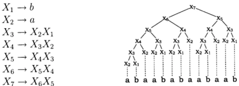
equal to its number of productions. An example SLP is illustrated in Figure 2-3.

X2 -a X5 X3 - X2X1 \ \ I\ X4 X3 X3 X2 X3 X2 X2 Xi X4 -- X3X2 /\ /\ /\ i /\ " ' X3 X2 X2 Xi X2 X X2 X X5 -+ X4X3 I \ X6 -+X5X4 : X7 X6X 5 a ba a a a a a b

Figure 2-3: Consider the string abaababaabaab. It could be generated by the above SLP, also known as the Fibonacci SLP.

transformed to straight-line programs quickly and without large expansion. In particular, consider

an LZ77 encoding [104i] with n" blocks for a text of length n. Rytter's algorithm produces an SLP-representation with size n' = O(n" log n) of the same text, in O(n') time. Moreover, n'

lies within a log n factor from the size of a minimal SLP describing the same text. Note also

that any text compressed by the LZ78 encoding can be transformed directly into a straight-line

program within a constant factor. However, here we focus our SLP example on LZ77 encoding

since in certain cases LZ77 is exponentially shorter than LZ78, so even with the log n degradation

associated with transforming LZ77 into an SLP, we may still get an exponential speedup over LZ78

from Section 2.3.3.

We next describe how to use SLP to achieve the speedup.

(I) Dictionary Selection: let X be an SLP representation of the input sequence. We choose

all strings corresponding to nonterminals X1,..., X,, as good substrings.

(II) Encoding: compute M(Xi) in the same order as in X. Every concatenating rule requires

just one max-times multiplication.

(III) Parsing: Trivial (the input is represented by the single matrix representing X,,).

(IV) Propagation: vt = M (X,,) 0 vo.

Time and Space Complexity. Let n' be the number of rules in the SLP constructed in the parsing

step (r = n/n' is the ratio of the grammar-based compression). The parsing step has an O(n) time

complexity and is computed offline. The number of max-times multiplications in the encoding step

is n'. Therefore, the overall complexity of decoding the HMM is n'k3, leading to a speedup factor

of

Q().

In the next section we give another example of a grammar-based compression scheme where

the size of the uncompressed text may grow exponentially with respect to its description, and that furthermore allows, in practice, to shift the Encoding Step (III) to an off-line preprocessing stage,

2.3.5

Acceleration via Byte-Pair Encoding

In this section byte pair encoding is utilized to accelerate the Viterbi decoding computations by

a factor of Q(r), where n' is the number of characters in the BPE-compressed sequence X and

r = n/n' is the BPE compression ratio of the sequence. The corresponding pre-processing term

for encoding is O(IE'|k3), where E' denotes the set of character codes in the extended alphabet.

Byte pair encoding [ , , ] is a simple form of data compression in which the most common

pair of consecutive bytes of data is replaced with a byte that does not occur within that data. This

operation is repeated until either all new characters are used up or no pair of consecutive two

char-acters appears frequently in the substituted text. For example, the input string ABABCABCD

could be BPE encoded to XYYD, by applying the following two substitution operations: First

AB -+ X, yielding XXCXCD, and then XC -+ Y. A substitution table, which stores for

each character code the replacement it represents, is required to rebuild the original data. The compression ratio of BPE has been shown to be about 30% for biological sequences [ ].

The compression time of BPE is O(lE'ln). Alternatively, one could follow the approach of

Shibata et al. [ , ], and construct the substitution-table offline, during system set-up, based on

a sufficient set of representative sequences. Then, using this pre-constructed substitution table, the

sequence parsing can be done in time linear in the total length of the original and the substituted

text. Let a E E' and let W, denote the word represented by a in the BPE substitution table. The four-step framework described in Section 2.2 is applied as follows.

(I) Dictionary Selection: all words appearing in the BPE substitution table are good sub-strings, i.e. D = {W, } for all a E E'.

(II) Encoding: if a is a substring obtained via the substitution operation AB -+ a then

M (W) = M (WA) 0 M(W).

So each matrix can be computed by multiplying two previously computed matrices.

(IV) Propagation: run VA on X', using the matrices M(Wi) as described in Section 2.2.

Time and Space Complexity. Step I was already taken care of during the system-setup stage

and therefore does not count in the analysis. Step II is implemented as an offline, preprocessing

stage that is independent of the observed sequence X but dependent on the training model. It can

therefore be conducted once in advance, for all sequences to come. The time complexity of this

off-line stage is O(IE'l1k3) since each matrix is computed by one max-times matrix multiplication

in O(k3 ) time. The space complexity is O(IE'1k2). Since we assume Step III is conducted in

pre-compression, the compressed decoding algorithm consists of just Step IV. In the propagation step

(IV), given an input sequence of size n, compressed into its BPE-encoding of size n' (e.g. n' = 4

in the above example, where X = ABABCABCD and X' = XYYD), we run VA using at most

n' matrices. Since each VA step takes k2 time, the time complexity of this step is O(n'k2). Thus,

the time complexity of the BPE-compressed decoding is O(n'k2) and the speedup, compared to

the O(nk2) time of VA, is Q(r).

2.4 Optimal state-path recovery

In the previous section, we described our decoding algorithms assuming that we only want to

compute the probability of the optimal path. In this section we show how to trace back the optimal path, within the same space complexity and in O(n) time. To do the traceback, VA keeps, along

with the vector vt (see eq. (2.2)), a vector of the maximizing arguments of eq. (2.2), namely:

ut+1[i] = argmaxj{P,j, vt[j]} (2.8)

It then traces the states of the most likely path in reverse order. The last state sn is simply the

largest element in vn, argmaxj {vn[j]}. The rest of the states are obtained from the vectors u by

st-1 = ut [st]. We use exactly the same mechanism in the propagation step (IV) of our algorithm.

The problem is that in our case, this only retrieves the states on the boundaries of good substrings but not the states within each good substring. We solve this problem in a similar manner.

Note that in all of our decoding algorithms every good substring W is such that W = WAWB

where both WA and WB are either good substrings or single letters. In LZ78-accelerated decoding,

WB is a single letter, when using RLE WA = WB = rlwl/2, SLP consists just of production

rules involving a single letter or exactly two non-terminals, and with BPE WA, WBE E Z'. For this

reason, we keep, along with the matrix M(W), a matrix R(W) whose elements are:

R(W),j = argmaxk{M(WA)i,k D M(WB)k,j} (2.9)

Now, for each occurrence of a good substring W = w1,. .. , we we can reconstruct the most

likely sequence of states si, , .. se as follows. From the partial traceback, using the vectors u,

we know the two states so and se, such that so is the most likely state immediately before wl was

generated and se is the most likely state when we was generated. We find the intermediate states

by recursive application of the computation sjwI = R(W)8,Os.

Time and Space Complexity. In all compression schemes, the overall time required for

trac-ing back the most likely path is O(n). Stortrac-ing the matrices R does not increase the basic space

complexity, since we already stored the similar-sized matrices M(W).

2.5

The Training Problem

In the training problem we are given as input the number of states in the HMM and an observed

training sequence X. The aim is to find a set of model parameters 0 (i.e., the emission and

transi-tion probabilities) that maximize the likelihood to observe the given sequence P(XI 0). The most

commonly used training algorithms for HMMs are based on the concept of Expectation

Maximiza-tion. This is an iterative process in which each iteration is composed of two steps. The first step solves the decoding problem given the current model parameters. The second step uses the results of the decoding process to update the model parameters. These iterative processes are guaranteed to converge to a local maximum. It is important to note that since the dictionary selection step

need run them once, and repeat just the encoding step (II) and the propagation step (IV) when the decoding process is performed in each iteration.

2.5.1 Viterbi training

The first step of Viterbi training [l3] uses VA to find the most likely sequence of states given the

current set of parameters (i.e., decoding). Let Aij denote the number of times the state i follows

the state j in the most likely sequence of states. Similarly, let Ei (a) denote the number of times the letter a is emitted by the state i in the most likely sequence. The updated parameters are given

by:

P = and ei(a) - (2.10)

PJ t Aij E,, EZ(a')

Note that the Viterbi training algorithm does not converge to the set of parameters that maximizes

the likelihood to observe the given sequence P(X 10) , but rather the set of parameters that locally

maximizes the contribution to the likelihood from the most probable sequence of states [30]. It is

easy to see that the time complexity of each Viterbi training iteration is O(k2n + n) = O(k2n) so

it is dominated by the running time of VA. Therefore, we can immediately apply our compressed

decoding algorithms from Section 2.3 to obtain a better running time per iteration.

2.5.2 Baum-Welch training

The Baum-Welch training algorithm converges to a set of parameters that maximizes the

likeli-hood to observe the given sequence P(X 0), and is the most commonly used method for model

training. Recall the forward-backward matrices: ft[i] is the probability to observe the sequence

xl, x2, ... , xt requiring that the t'th state is i and that bt[i] is the probability to observe the

se-quence Xt+1, t+2,..., an given that the t'th state is i. The first step of Baum-Welch calculates ft [i] and bt [i] for every 1 < t < n and every 1 < i < k. This is achieved by applying the forward