Aerodynamic measurement and analysis of the flow in an uncooled turbine stage

AERODYNAMIC MEASUREMENT AND ANALYSIS OF THE FLOW IN AN UNCOOLED TURBINE STAGE

by

LEo M. GREPIN

B. Eng. Honours Mechanical Engineering, McGill University (1996)

Submitted to the Department of Aeronautics and Astronautics in partial fulfillment of the requirements for the degree of

MASTER OF SCIENCE at the

MASSACHUSETTS INSTITUTE OF TECHNOLOGY June 1998

©

Author

D nent of Aeronautics and Astronautics May 15, 1998

Professor Alan H. Epstein R. C. Maclau(in Professor of Aeronautics and Astronautics Thesis Supervisor

Professor Jaime Peraire Associate Pofessor of Aeronautics and Astronautics Chair, Graduate Office

..

". :i

.AERO

..

Accepted by

AERODYNAMIC MEASUREMENT AND ANALYSIS OF THE FLOW IN AN UNCOOLED TURBINE STAGE

by

LEo M. GREPIN

Submitted to the Department of Aeronautics and Astronautics on May 15, 1998, in partial fulfillment of the

requirements for the degree of Master of Science

ABSTRACT

This thesis is part of an effort to develop new instrumentation techniques for blowdown turbine testing. Two experimental methods used to study turbine aerodynamics in the MIT Blowdown Turbine Facility are presented:

Differential pressure measurement - The high accuracy performance study of a turbine stage motivated research in mass flow measurement techniques in a blowdown environment. A combination of total and differential pressure and total temperature measurements was used to calculate the mass flow per unit area through the turbine stage. The design of a new differential pressure probe was a critical component of the research effort. Measurement uncertainties of less than 1% were required while operating near the sensor burst pressure. The mass flow measurements, accurate to 1%, served to validate mass flow measurements simultaneously acquired using a Venturi nozzle mass flow meter.

Particle Image Velocimetry - A successful application of particle image velocimetry in a fully-scaled rotating turbine rig is presented. The image processing procedure is described and the results are assessed using a comparison with a numerical solution. The CFD code used is a coupled Navier-Stokes/Euler 2-D solver with rotor/stator interaction. Differences of 20 to 60% between CFD and PIV local velocities were partially explained by modeling the motion of seeding particles in the turbine stage and assessing the influence of particle di-ameter on PIV accuracy. For the present application, 0.5 im was found to be the maximum seeding particle size for tracking errors of less than 5%. The PIV results supported previous research in predicting substantial aperiodic unsteadiness in the rotor/stator passage.

Thesis Supervisor: Professor Alan H. Epstein

ACKNOWLEDGMENTS

I would like to express my gratitude to Professor Alan Epstein and Dr. Gerald Guenette, for their guidance, encouragement and insightful suggestions throughout this work.

I am greatly indebted to: Lori Martinez, Holly Anderson, Bob Haimes, Viktor Dubrowski, Mariano Hellwig, James Letendre, Tom Ryan and Bill Haimes, for their invaluable admin-istrative and technical support.

I am grateful to the students who worked with me on the Blowdown Turbine for always being helpful and for sharing with me explosions of joy and explosions of equipment: Rory Keogh, Jason Jacobs, Yi Cai and Chris Spadaccini.

I would like to thank all the friends who made my MIT experience unforgettable. Namely, Amit and Arnaud, for corrupting me into playing golf on busy week-ends; Luc for sharing with me memories of "poutine" and thoughts on life; Rory for our heated discussions on the "Wild,Wild West" and world issues; Zolti, for being more of a brother than a roommate to me; "les potes francais", Jeremie, Sophie, Omar and Ahmed for putting a little bit of France in the Boston sky, and finally all the people at the GTL for making everyday an interesting one.

Finally, I thank my family; you guided me, helped me, supported me without ever crit-icizing my decisions; you are my motivation and drive.

And Anna, my Love for you is behind every word in this thesis.

This project was sponsored by the US Air Force Office of Scientific Research Grant F49620-96-1-0266. Their support is gratefully acknowledged.

CONTENTS

1.4 The MIT Blowdown Turbine Test Facility . . . . 1.5 Organization of the Thesis ...

2 Measurement of Dynamic Pressure

2.1 Introduction ... .. .. .. ... .. .. ... . 2.2 Constraints on Differential Pressure Instrumentation 2.3 Design of the Differential Pressure Probe . . . . 2.4 Experimental Set-Up ...

2.5 Calibration Sequence ...

2.6 Applications of Dynamic Pressure Measurements . . 2.7 Validation of Experimental Procedure . . . . 2.8 R esults . . . . 2.9 Chapter Summary ...

3 Non-Intrusive Study of Turbine Flow: Particle Image 3.1 Introduction ...

3.2 Flow Visualization using Particle Image Velocimetry .. 3.2.1 Pulsed-Light Velocimetry . ... Velocimetry 19 . . . . 19 . . . . 20 . . . . 21 . . . . . 22 . . . . 24 27 . . . . 27 . . . . . 28 . . . . . 30 . . . . 34 . . . .. . 35 . . . . . 36 . . . . . 38 . . . . 39 . . . . 41

3.2.2 Particle-Image Velocimetry ... 3.3 Experimental Set-Up ...

3.3.1 Test Facility .... ... ... 3.3.2 Optical System ...

3.3.3 Particle Seeding ... 3.4 Image Processing Algorithm ...

3.4.1 Digitized PIV Images ... 3.4.2 Autocorrelation ... 3.4.3 Image Calibration ...

3.4.4 Generation of the Velocity Flow field . 3.4.5 Test Conditions ...

3.5 R esults . . . . 3.6 Chapter Summary ...

4 Numerical Modeling of the Flow through the ACE Turbine 4.1 Introduction . . . . 4.2 Numerical Model (UNSFLO) ...

4.3 Assessment of the UNSFLO Code . . . . 4.4 Computational Procedure ...

4.5 Initial Conditions ... 4.6 Results ...

4.7 Sensitivity of the Flow to Variations in Computational Parameters 4.7.1 Sensitivity to Boundary Conditions . ...

4.7.2 Sensitivity to Rotor/Stator Relative Position ... 4.8 Chapter Summary ...

5 Comparison of PIV Measurements with CFD Results 5.1 Introduction ...

5.2 Comparison of the Velocity Fields . . ... 5.2.1 General Features ...

5.2.2 Comparison of Velocity Profiles . . . . 5.2.3 Conclusions of the Comparison . ...

5.3 Particle Dynamics ... . . . . 49 . . . . 5 1 . . . . 5 1 . . . . 52 . . . . . 52 . . . . 53 . . . . 53 . . . . 54 . . . . 54 . . . . . 55 . . . . 58 . . . . . 58 . . . . 59 65 65 65 66 67 68

5.3.1 Theory of Dusty Gases . . . .. 5.3.2 Particle Path Model ...

5.4 R esults . . . . 5.4.1 Particle Dynamics in the Rotor Passage . . . . 5.4.2 Particle Dynamics in the Stator Vane Passage . 5.4.3 Influence of Particle Rotor Inlet Conditions . . 5.4.4 Particle Size Estimation . . . . 5.5 Evaluation of PIV Results . . . . 5.6 Chapter Summary ...

6 Conclusions

6.1 Summary of the Research . . . . 6.2 Contributions of the Work . . . . 6.3 Recommendations for Future Work . . . .

A Aerodynamic Measurement Error Analysis A.1 Introduction ...

A.2 Measurement Error ... A.2.1 Precision Error ... A.2.2 Bias Error ...

A.2.3 Degrees of Freedom in Error Sources A.3 Propagation of Uncertainty ...

A.4 Pressure and Temperature Measurements . A.5 Uncertainty in Mach Number Calculations . A.6 Uncertainty in Mass Flow Calculations . . . A.7 Summary ... B PIV B.1 B.2 B.3 113 . . . 113 . . . 113 . . . 114 . . . 114 . . . . . 115 . . . 115 . . . . . 116 . . . . . 118 . . . . . 119 . . . 120

Measurement Error Analysis Introduction . . . . Sources of Uncertainty ... ... Sum m ary . . . . Bibliography 121 121 121 124 125 . . . . . . 84 . . . . 86 . . . . 88 . . . . . . 88 . . . . . . 90 . . . . . . 90 . . . . . . 91 . . . . . . 92 . . . . 94 109 109 110 111

LIST OF FIGURES

The MIT Blowdown Turbine Facility . ... The MIT Blowdown Turbine Facility flow path . ...

Uncertainty estimate for differential pressure measurements . . . ... Dynamic pressure measurement during test start-up transient ... Schematic of the dynamic pressure probe . ...

Power spectra of the pressure probe signals upstream of the turbine . Schematic of a single expansion chamber silencer . ... Schematic of the mass flow probe ...

Turbine mass flow as a function of time . ... Mass flow probe pressure and temperature signals ...

Time history of Mach number for low and high Reynolds number tests . Time history of corrected mass flow for low and high Reynolds number tests

Digitized image of the PIV calibration grid . . . . Digitized PIV picture ...

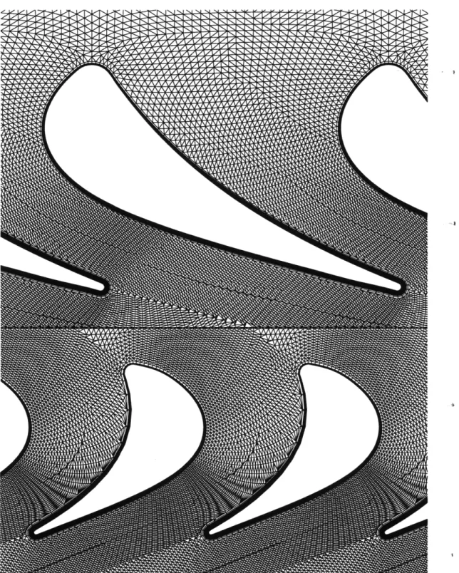
Detail of a PIV picture showing three particle pairs . . . . Image processing algorithm for PIV images . . . . Optical system for particle-image velocimetry experiments . . . Schematic view of the laser light sheet plane . . . . PIV solution at the midspan of the ACE turbine rotor passage Close-up of rotor passage exit PIV solution . . . . 4-1 Computational grid used to model the flow through the ACE turbine. 4-2 Velocity map for the rotor passage in the rotor relative frame . . . . . 4-3 Convection of the stator wake in the rotor passage . . . . 4-4 Time-unsteady shock patterns in the ACE turbine stage . . . . 4-5 Streamline height for quasi-3D model . . ...

1-1 1-2 2-1 2-2 2-3 2-4 2-5 2-6 2-7 2-8 2-9 2-10 3-1 3-2 3-3 3-4 3-5 3-6 3-7 3-8 . . . . . 55 .... . 56 . . . . . 57 . . . . . 62 . . . . . 62 . . . . . 63 . . . . . 64 . . . . . 64

Schematic of the rotor passage ...

Velocity profiles in a single rotor passage for extreme initial conditions . Schematic of 5 rotor/stator index positions . ...

Velocity profiles in a single rotor passage for 5 different rotor/stator indices 4-6 4-7 4-8 4-9 5-1 5-2 5-3 5-4 5-5 5-6 5-7 5-8 5-9 5-10 5-11 5-12 5-13 5-14 5-15 5-16

Composite diagram of the velocity profiles in the Axial CFD velocity profiles and comparison with Axial CFD velocity profiles and comparison with Axial CFD velocity profiles and comparison with Axial CFD velocity profiles and comparison with Axial CFD velocity profiles and comparison with Axial CFD velocity profiles and comparison with Fluid streamlines and particle trajectories in the Particle axial and circumferential velocity deficit Particle axial and circumferential velocity deficit Particle axial and circumferential velocity deficit Particle axial and circumferential velocity deficit

rotor passage PIV results (1) PIV results (2) PIV results (3) PIV results (4) PIV results (5) PIV results (6) rotor passage in the rotor passage in the rotor passage in the rotor passage in the rotor passage

.. . . . . 92 .. . . . . 93 .. . . . . 96 .. . . . . 97 . . . . . . 98 . . . . . . 99 . . . . . . 99 . . . . . . 99 . . . . . . 100 . . . . . . 100 . . . . . . 100 .. . . . . 101 (1) . (2) . (3) . (4) . 5-17 Fluid streamlines and particle trajectories in the stator passage . . . . 5-18 Axial and circumferential velocity deficit in the stator passage . . . . 5-19 Influence of particle initial conditions on motion in the rotor passage . . .. 5-20 Particle axial and circumferential velocity history in the rotor passage (1) 5-21 Particle axial and circumferential velocity history in the rotor passage (2)

102 102 103 103 104 105 106 107 108 Styrene particle diameter distribution for a typical PIV test .

Particle motion on the suction side of the rotor blade . . . . . Comparison of CFD and PIV flow fields (1) . . . . Comparison of CFD and PIV flow fields (2) . . . .

.

.

.

LIST OF TABLES

1.1 Ground based turbine stage scaling in the MIT Blowdown Turbine Facility 23

2.1 Specifications of the pressure sensors ... ... 31

2.2 Average Mach number measurements ... ... 39

2.3 Average effective area measurements ... ... 41

3.1 ACE turbine stage scaling in the MIT Blowdown Turbine facility ... 51

3.2 Seed particle properties in the PIV experiments . ... 53

3.3 Experimental conditions for the PIV images . ... 61

4.1 Computational parameters for the CFD calculations . ... 72

A.1 Propagated uncertainty in Mach number measurements . ... 118

A.2 Propagated uncertainty in Mass flow measurements . ... 120

B.1 Statistics from the calibration of the PIV optical set-up . ... 122

NOMENCLATURE

Roman

a speed of sound ( -yRT) [m/s]

Ac frontal area of seed particle [m2

]

Aeff _{effective area [m}2

] CD drag coefficient

Cp mass specific heat capacity at constant pressure [J/kg.K]

d seed particle diameter [m]

D diameter [m]

L length [m]

m mass [kg]

M Mach number (l)

n number of statistical samples

P pressure [Pa]

6P dynamic pressure [Pa]

Rgas gas constant [J/kg.K]

s curvilinear coordinate [m]

S1 Sutherland's temperature constant [K]

t time [s]

T temperature [K]

u _{axial component of velocity [m/s]}

v circumferential component of velocity [m/s]

V volume of seed particle [m3

]

V velocity vector [m/s] x axial location [m]

X Cartesian position vector [m]

y circumferential location [m]

Greek

"I ratio of specific heats E measurement uncertainty

0 rotor inlet flow angle (from axial) K rotor/stator index

P dynamic viscosity [kg/m.sec] 7r turbine pressure ratio

p density [kg/m 3]

T torque [N.m]

w turbine angular speed [rad/s]

Superscripts

derivative with respect to time

Subscripts

f fluid particle property

p seed particle property

t stagnation (or total) fluid quantity

1 supply tank

CHAPTER

1

INTRODUCTION

1.1

Background

The globalization and deregulation of the aeronautical industry in the last few decades has forced industry players to compete both on quality and price. The consequence of this has been two fold. Incremental improvements in technology have become crucial for competitive advantage and the budgets feeding the research have shrunk drastically. In the commercial and military industry, most development projects have evolved to include few test rigs. In the power generation industry where the engines and power requirements are large, components are tested in service.

This evolution in the research and development of gas turbine engines was made possible by advances in computer power and design tools such as computational fluid dynamics (CFD) and CAD/CAM programs. Certain design steps, however, still rely on empirical approaches. For example, the trade-offs involved in the design of cooled turbines have yet to be captured by computational tools and significant testing is still necessary during the development of a new engine.

To replace steady test rigs, short-duration transient facilities were developed in the 1980's to study components of gas turbine engines at fractions of the energy requirements and construction costs. The MIT Blowdown Turbine test rig is such a facility. It has been successfully used to study, amongst other things, the effect of inlet temperature distortions on turbine heat transfer and the impact of film cooling on heat transfer and efficiency.

This thesis focuses on demonstrating the feasibility of new applications in a blowdown environment. Namely, the design of a dynamic pressure probe is investigated along with its suitability for inferring Mach number and mass flow when combined with stagnation pressure and temperature sensors. Also, particle-image velocimetry (PIV) is studied as a candidate for obtaining instantaneous flow fields in a transient environment by non-intrusive means.

1.2

Literature Review

The MIT Blowdown Turbine Facility was one of the first short duration turbomachinery experiments developed in the early 1980's. Papers by Epstein [14] and Guenette [20] present the issues involved in the design of such a facility. The importance of time and physical scales is thoroughly discussed as well as the instrumentation required in unsteady short-duration testing.

During the past fifteen years, the MIT blowdown turbine facility has been successfully used to study key phenomena affecting turbine flow:

1. The effect of film cooling on blade heat transfer was investigated by Abhari [1] by measuring the heat transfer coefficient on the blade surface for cooled and uncooled blades. The results obtained in the blowdown turbine rig were compared to results obtained in a cascade facility and the unsteady nature of the cooling process was studied using a mathematical model.

2. The effect of inlet temperature distortions on turbine heat transfer was studied by Shang [27] in conditions typical of combustor exit flows. Radial temperature dis-tortions were found to have a profound influence on blade heat transfer while cir-cumferential distortions did not. The experimental study was complemented by a computational investigation of the mechanisms driving rotor blade surface heat trans-fer.

3. The latest research focuses on the effects of film cooling on turbine performance. The research was undertaken by Keogh [24] and Cai [9]. Most of the early efforts focused on developing instrumentation to accurately monitor the facility as efficiency

calculations require low-uncertainty measurements of mass flow, shaft torque, pressure and temperature.

1.3

Motivation and Objectives

The main motivation behind this work is the need for more accurate and complete tools to study, in a blowdown facility, the factors affecting turbine flow. More specifically, two experimental methods are examined as candidates to further the flexibility of transient turbine testing:

1. The measurement of dynamic pressure: Dynamic pressure measurements can be com-bined with total pressure and temperature measurements to infer Mach number and mass flow. The challenge in a blowdown environment is to accurately capture changes in differential pressure that are fractions of percents of the common mode pressure. In addition, the common mode pressure varies during a test between vacuum and several atmospheres, creating tremendous stress on the sensor.

2. Particle-image velocimetry: PIV can generate instantaneous velocity fields for un-steady flows. if the concept of PIV can be validated for turbomachinery flows, it would have many applications: at the design stage, the results can be used to fine tune blade shapes for unsteady effects, at the academic level, they can be used as a reference to validate CFD codes or to investigate unsteady effects in turbines.

As such, the specific objectives of this thesis are as follows:

1. To demonstrate the feasibility of a dynamic pressure probe in a blowdown environ-ment.

2. To bound the accuracy of Mach number and mass flow calculations obtained from pressure and temperature measurements in a short-duration, transient experiment. 3. To demonstrate the feasibility and the potential of particle image velocimetry for

4. To quantify the difference between PIV and CFD solutions for the flow through the Rolls-Royce ACE turbine.

5. To identify the sources of discrepancies between the PIV and CFD results.

1.4

The MIT Blowdown Turbine Test Facility

This section describes the facility used for the acquisition of the experimental data contained in this thesis. The MIT Blowdown Turbine Facility is a fully scaled short duration transient wind tunnel. A detailed explanation of the design and operation of the facility can be found in references [14] and [20]. The following is a brief description of the operating concepts.

A blowdown turbine experiment rigorously simulates the operational environment of a transonic engine turbine stage: (1) the properties of the flow (pressure, temperature, mass flow) change throughout a test but the non-dimensional parameters governing fluid dynamic and heat transfer phenomena remain constant; (2) the time-scales of the flow and the rotor to stator passing frequency are much smaller than the test time of approximately 500 ms so that the turbine operates in a quasi-steady state similar to the steady state operation of an engine.

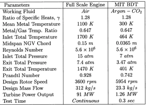
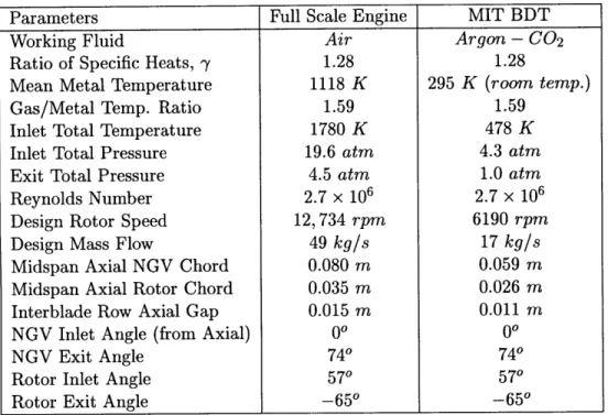
The test stage is a scaled down version of the stage in the full engine. Table 1.1 presents the characteristics of the 2:1 pressure ratio ground based turbine stage used for the devel-opment of the mass flow probe described in Chapter 2. The particle image velocimetry experiment, discussed in Chapter 3 was conducted on a 4:1 pressure ratio turbine stage, the scaling parameters of which are summarized in Table 3.1.

The choice of the test gas and of its initial conditions is based on the need to match relevant non-dimensional parameters and to maximize the safety of the facility. Argon and

C02 are used in the experiments presented in this thesis. Due to the high density of the

working gas, the Reynolds number similarity can be achieved at low pressure and, due to the high density, the tip Mach number similarity can be satisfied at a fairly low Mach number. The mixture ratio is set to match the specific heat ratio, y, of the full-scale turbine.

A schematic of the blowdown turbine facility is presented in figure 1-1. The main components are the supply tank, the fast acting valve, the test section, the downstream

Parameters Full Scale Engine MIT BDT

Working Fluid Air Argon - CO2

Ratio of Specific Heats, y 1.28 1.28

Mean Metal Temperature 1100 K 300 K

Metal/Gas Temp. Ratio 0.647 0.647

Inlet Total Temperature 1700 K 464 K

Midspan NGV Chord 0.15 m 0.0365 m

Reynolds Number 5.6 x 106 5.6 x 106

Inlet Total Pressure 15 atm 7 atm

Exit Total Pressure 7.4 atm 3.47 atm

Exit Total Temperature 1470 K 401 K

Prandtl Number 0.928 0.742

Design Rotor Speed 3600 rpm 5954 rpm

Design Mass Flow 312 kg/s 23.3 kg/s

Turbine Power Output 91 MW 1.26 MW

Test Time Continuous 0.3 sec

Table 1.1: MIT blowdown turbine scaling for a ground based turbine stage at design point.

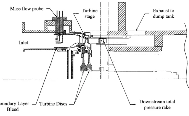
translator and the dump tank. The cross sectional view of the test section, in figure 1-2, shows the flowpath and some of the instrumentation.

During a blowdown test, the facility is pumped down to vacuum and the supply tank is heated to the desired temperature. The fast acting valve is closed and the supply tank is filled to test pressure. All the pressure sensors undergo a post-fill calibration. After setting the data acquisition system, translator and eddy current brake to standby mode, the rotor is spun up in vacuum by a drive motor to a speed slightly above the test speed. The drive motor is shut off and the rotor slows down due to friction in the bearings. When the rotor speed reaches the test speed, the fast acting valve opens in 20-50 ms and the eddy current brake, translator and data acquisition system are triggered. The test gas from the supply tank enters a contraction which simulates the combustor exit upstream of the nozzle guide vanes. Boundary layer bleeds are located upstream of the contraction and ensure a uniform velocity profile at the inlet of the test section. The turbine pressure ratio is set by a throttle plate downstream of the test section. Start-up transients decay in about 200 ms and are followed by 500-800 ms during which the throttle plate remains choked. For the 2:1 pressure ratio turbine tests, the first 1000 ms of data are acquired at 3.03 kHz. The facility is then monitored at 1 Hz for 9 min to track the decay of the flow and to conduct post-test sensor calibrations.

1.5

Organization of the Thesis

This chapter introduces the content of the thesis, presents previous research undertaken in a blowdown environment, outlines the motivations behind this research and describes the characteristics of the MIT blowdown turbine facility.

Chapter two treats the need for and complexity of differential pressure measurements in a blowdown environments. A method for inferring Mach number and mass flow from flow property measurements is presented along with its implementation and the results of the tests.

Chapter three presents some of the first data obtained in rotating turbomachinery using Particle Image Velocimetry (PIV). The experimental apparatus and the image processing algorithm are described, along with the results of the particle image velocimetry experi-ments.

In chapter four, Computational Fluid Dynamics (CFD) results are presented as a basis for comparison with the PIV data. The numerical algorithm used is described, as well as the details of the calculations.

Chapter five is a comparison between the results of the two previous chapters. It presents the agreement of the experimental and computational solutions to the flow field through the ACE turbine and discusses sources of discrepancies.

Salve

Figure 1-1: The MIT Blowdown Turbine Facility.

Inlet

Boundary Layer J Turbine Discs

J/

\

Bleed pressure rake

CHAPTER

2

MEASUREMENT OF DYNAMIC

PRESSURE

2.1

Introduction

Testing in a short-duration transonic tunnel requires high accuracy and fast response instru-ments. Static and total pressure sensors have been refined over the years and are accurate to within 1% or better [24]. Dynamic pressure on the other hand is difficult to measure in a transient environment and has received little attention. The challenge arises from the nature of a blowdown test: the dynamic pressure sensor must be capable of measuring pressure fluctuations on the order of a hundredth of a psi while at the same time surviving a start-up transient of a few milliseconds during which the ambient pressure in the tunnel rises from vacuum to values in excess of 100 psi. A probe designed to overcome the above technical challenge has many applications. Dynamic pressure measurements can be used to infer flow properties such as Mach number, mass flow and efficiency.

This chapter presents research contributing to a series of experiments on a 2:1 pressure ratio turbine stage. The purpose of the testing is to generate high accuracy (less than 1% uncertainty) performance data for the uncooled and cooled version of the turbine stage. As part of this effort, several techniques for measuring mass flow were investigated. The combination of total and dynamic pressure and total temperature measurements was one of the options. The requirements of a dynamic pressure probe, its feasibility and its suitability for the aforementioned applications is discussed below.

2.2

Constraints on Differential Pressure Instrumentation

The design of the differential pressure probe and its feasibility are based on three require-ments: accuracy, time response and robustness.

Accuracy

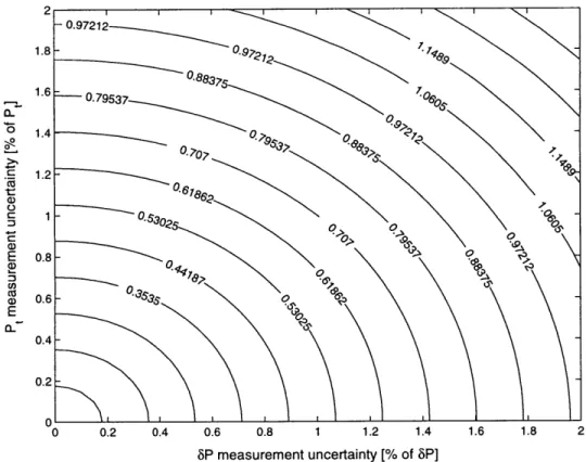
Differential pressure measurements are useful if they can be combined with total pressure and total temperature measurements to infer mass flow and Mach number. The target uncertainty for the mass flow measurements in these experiments is 1% or less. This figure was used as an upper bound in the design of the differential pressure probe. A first order estimate for the accuracy requirement of the differential probe was calculated assuming experimental uncertainty in the total pressure and differential pressure measurements only. The mass flow uncertainty is then given by:

E2t+ (66 22

= 6+ (2.1)

rh rh

where rh is defined as in Equation 2.4.

Figure 2-1 is a contour plot of the percentage uncertainty in mass flow as a function of the percentage uncertainty in Pt and JP. The total pressure measurement is expected to be accurate to within 1% (cf. Appendix A). Using a conservative estimate, an uncertainty level of 1% or less for the differential pressure measurements ensures a propagated uncertainty of less than 1% for the inferred mass flow calculations.

Time Response

The second design constraint is the time response of the instrument. A pressure transducer time response of 1 ms is sufficient to track the overall behavior of the flow during the steady operation of the rig. During the start-up transient, however, the probe is subjected to a pressure step and must stabilize quickly in order to accurately measure the flow during the quasi-steady portion of the expansion process. Putting this in perspective with the time scale of the test, the effects of the initial pressure peak on the probe must have decayed in

1.6 - 0.79537 ₀ 0 1.4 ₀ .C 1.2 19 0.6186 00 Co 1 E 0.8 3S 0.6 0.2 0 0.2 0.4 0.6 0.8 1 1.2 1.4 1.6 1.8 2 8P measurement uncertainty [% of 5P]

Figure 2-1: Percentage uncertainty in mass flow calculations due to uncertainty in total and

differential pressure measurements.

a few dozen milliseconds.

Probe Robustness

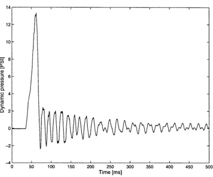
The final concern in the design of the dynamic pressure probe is its ability to survive the start-up transient that follows the opening of the fast-acting valve. To estimate the dynamic pressure to which the sensor is subjected during the passage of the expansion wave in the tunnel, a Pitot static probe was connected to a 100 psi differential pressure sensor during a blowdown test at 50 psi. The results of the test are presented in Figure 2-2. They show that the differential sensor must survive a few millisecond exposure to a differential pressure on the order of 15 psi.

12 - 10- 8-CL 2₄ --2 -41 0 50 100 150 200 250 300 350 400 450 500 Time [ms]

Figure 2-2: Plot of the dynamic pressure during the start-up transient of a test with initial pressure of 50 psi.

2.3

Design of the Differential Pressure Probe

The differential pressure probe was designed based on the three criteria described above. The probe consists of three components: the Pitot static tube, the pressure sensor and the calibration equipment.

Pitot Static Tube

The Pitot static tube was chosen based on its time-response, its accommodation to mis-alignment with the flow and its size to minimize the disturbances on the downstream flow. A 1/8" diameter United Sensor Pitot-static probe was chosen (cf. Figure 2-6). Empirical tests concluded that a 50 misalignment contributes to less than 0.5% error in the measure-ment. The disturbance to the turbine stage inlet flow forty probe diameters downstream are expected to be negligible.

The time response of the tube and its connections to the sensor was calculated based on the work of Grant [19]. For a probe subjected to a step change in pressure, the probe

Sensor 6P 6P calibration Pt

Manufacturer Kulite Setra Kulite

Model XCS - 062 - 5D 228 - 1 XCQ - 062 - 100D

Pressure Range 0 to 5 psi D 0 to 1 psi D 0 to 100 psi D

Maximum overload 15 psi D 100 psi D 300 psi D

Time response - 40 ms

Nonlinearity +0.5%FS +0.2%FS +0.5%FS

Hysteresis 0.1% FS 0.2% FS 0.1% FS

Non-repeatability 0.1% FS +0.2% FS 0.1% FS

Overall accuracy ±0.5%FS ±0.25%FS ±0.5%FS

Resolution Infinite Infinite Infinite

Table 2.1: Specifications of the pressure sensors.

volume fills exponentially. The time constant for the process is: 128pLV

7 =

rD 4P (2.2)

where p is the dynamic viscosity of the fluid, L is the length of the probe, V is its volume,

D is the probe head orifice diameter and P is the pressure step.

T is the time required for 63% of the eventual response to the pressure step to occur. In 57, 99.3% of the response is achieved. This corresponds to 11 ms for the present probe design with a pressure step of 70 psi.

Differential Pressure Sensor

The pressure sensor was the most critical component of the design, with the following re-quirements: small internal volume for fast time response, low measurement uncertainty (1% or less) and high burst pressure (15 psi or higher). The Kulite 5 psi differential pressure sensor was found to be the most suitable candidate. In particular, it remains stable un-der pressures three times the full scale pressure, which was necessary during the start-up transient. Its characteristics are presented in table 2.1.

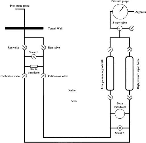
Pressure gauge Pitot static probe

S Argon supply

3-way valve

Tunnel Wall X

Run valve X X Run valve

Shunt 1

o 0

Kulite transducer

Calibration valve (X) (X) Calibration valve

Kulite X X Setra Setra transducer Shunt 2

Figure 2-3: Schematic of the dynamic pressure probe (all valves are manual).

Calibration Equipment

To control the Kulite sensor calibration, its gain was monitored before and after each test using a 1 psi differential Setra pressure gauge accurate to -0.25% of full scale. The accuracy of the calibration was maximized by performing it at the same common mode pressure as during the experimental tests. The specifications of the Setra transducer are presented in Table 2.1.

Figure 2-3 presents the main features of the differential pressure probe calibration set-up. The shunt valves were installed to prevent the differential pressure sensors from being exposed to a pressure above their burst pressure during the manipulation of the system before and after the test.

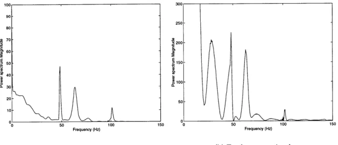
90 250-80 S70 200 S60 EE 50 150-40 30 20 ₅₀ 10-0 50 100 150 0 50 100 150 Frequency (Hz) Frequency (Hz)

(a) Dynamic pressure signal (b) Total pressure signal

Figure 2-4: Power spectra of the pressure probe signals upstream of the turbine.

Complete Dynamic Pressure Probe

Several versions of the dynamic pressure probe were tested. The main problem with the measurement was the high level of oscillation in the signal. To determine if this was due to resonance in the cavities of the dynamic pressure probe, the frequency content of the total and dynamic pressure signals were compared (cf. Figure 2-4). Since the dominant frequencies in the signal of the dynamic pressure probe are also present in the signal of the total pressure probe, the vibrations are most likely a consequence of the sudden expansion process at start-up.

To damp out the vibrations, different size expansion chamber silencers were interposed between the Pitot tube and the Kulite sensor (cf. Figure 2-5). Because the orifice of the Pitot tube restricts the mass flow filling up the cavities leading to the Kulite sensor, there is a trade-off between damping the vibrations and decreasing the frequency response of the probe. It was found that the silencer necessary to suppress the dominant 50Hz frequency, decreased the response of the probe to 500 ms during the startup transient. The probe is required to respond in less than 15 ms so the silencer was not used in the final design.

Flow-Figure 2-5: Schematic of a single expansion chamber silencer. Maximum damping occurs at frequencies for which sin wL/c = ±1. The magnitude of the damping depends on the geometry of the silencer [12].

Mass Flow Probe

To complement the dynamic pressure measurements, a stagnation pressure probe and a stagnation temperature probe were mounted beside the Pitot probe (cf. Figure 2-6). For the total pressure measurements, a 100 psi Kulite sensor was selected and connected to a 1/8" Venturi type Kiel probe (cf. Table 2.1). The mass flow probe is represented inserted in the flow path in Figure 1-2.

The total temperature probes use Omega 0.0005in diameter type K thermocouples lo-cated inside an impact probe. Their design was developed by Cai [9] and their uncertainty was demonstrated to be less than 0.05%.

In order to account for circumferential non-uniformities, three sets of probes were used and are referred to as probe A, probe B and probe C, respectively. They were installed 1200 apart and 600 from the structural struts at the inlet of the contraction. The probe heads were positioned at the annulus centerline.

2.4

Experimental Set-Up

The dynamic pressure instrumentation was developed to serve in the latest application of the blowdown turbine: the measurement of the influence of film-cooling on turbine per-formance. The facility used is a modified version of that presented in Section 1.4. The operating principles are the same but a Venturi mass flow meter has been added between

the test section and the dump tank. A complete description of the facility can be found in reference [24].

2.5

Calibration Sequence

To ensure the accuracy of the sensor calibrations and, hence of the measurements, all the instruments were calibrated before and after the experimental tests. This procedure was used to monitor the drift of the sensors due to the high pressure expansion wave during the start-up transient and the time stability from test to test. The calibration sequence is described below in detail.

Calibration of the differential pressure probes

Before and after the test, the Kulites were calibrated at the operating common mode pres-sure. The sensors have a linearity of ±0.5% FS and therefore a 2-point calibration was used between 0 psi differential and a differential of approximately 0.5 psi, the approximate pres-sure difference during the test. The Setra sensor was used as a reference for the differential pressure calibration.

During calibration, the tunnel is in vacuum for the pre-test calibration and at a pressure of several atmospheres for the post-test calibration. The run valves must be closed to isolate the calibration set-up from the run environment (cf. Figure 2-3). All other valves are open, in particular the shunt 1 and shunt 2 valves, whose function it is to protect the Kulite and Setra sensors from pressures above their burst pressure. The calibration system is pressurized to the expected working pressure during the test using the Argon supply. The

high and low pressure bottles are closed and the low pressure bottle is bled to 0.5 psi below

the pressure of the high pressure bottle. The data acquisition system is triggered. The zero differential of the sensors is monitored for two minutes after which the system is switched to differential mode: the shunt valves are closed to isolate the two sides of the Kulite and Setra sensors. The low and high pressure bottles are opened on the side communicating with the calibration system, yielding a pressure differential across the sensors. The differential is monitored for two minutes after which the system is brought back to zero differential by

opening the shunt valves and recording the sensor output for two more minutes.

Calibration of the total pressure probes

The total pressure sensors are also calibrated before and after the test. A pressure dif-ferential is applied between the reference pressure side of the Kulites and the sensing side, monitoring the tunnel conditions. For the pre-test calibration, the tunnel is in vacuum. The post-test calibration is performed after the tunnel has reached equilibrium. The calibration is executed by switching the reference pressure between atmosphere and vacuum. Since the pressure sensors are linear, a two point calibration is used to transform the voltage output of the sensors into engineering units.

Calibration of the total temperature probes

The total temperature sensors are calibrated in an oil bath monitored by NIST-traceable instruments. A fifth order polynomial is fitted through the multi-point calibration to yield an uncertainty of less than 0.05%. The calibration procedure is described in detail in reference [9].

2.6

Applications of Dynamic Pressure Measurements

Dynamic pressure measurements are valuable because in conjunction with stagnation pres-sure and temperature meapres-surements, they are used to calculate the Mach number and mass flow properties of the flow. These quantities in turn can be applied to inferring the me-chanical efficiency of the turbine stage under study. The details of these calculations are presented below.

Mach Number Calculations

The Mach number, M, in the contraction upstream of the turbine stage can be calculated from the compressible flow equations:

2

1

M =

*

- 1

(2.3)

- -1

Pt

t6P

where Pt is the stagnation pressure, 5P is the dynamic pressure and 7 is the ratio of specific heats.

Mass flow Calculations

The mass flow, rh, through the turbine facility can also be inferred using the compressible flow equations and the measurements at the upstream contraction:

S= Aeff Pt RM (2.4)

t

where Aeff is the effective area in the plane of the dynamic pressure probe in the upstream contraction and the other variables are as defined above.

Efficiency Calculations

The latest research efforts in the Blowdown Turbine Facility have been in the measurement of turbine performance in a blowdown environment. The measurement of thermodynamic efficiency was investigated by Cai [9] and the measurement of shaft efficiency by Keogh [24]. The latter is based on the measurement of the mass flow through the turbine and the torque on the turbine shaft. It is defined as the ratio of the actual power to the ideal power extracted from the turbine and, in its ideal gas form, can be expressed as:

S= W (2.5)

where T, W, Tt4, 7r, and Cp are the torque, angular speed, turbine inlet stagnation temper-ature, turbine pressure ratio and specific heat capacity, respectively.

2.7

Validation of Experimental Procedure

The prime goal of the experiments on the ground based turbine stage was to accurately mea-sure aerodynamic performance. The biggest challenge in achieving this goal was obtaining accurate mass flow measurements. This problem was studied at length by Keogh [24]. The most reliable mass flow measurement technique is to use a Venturi nozzle calibrated against NIST standards between the choking plate and the dump tank. This method gives re-sults accurate to within +0.25%. The technical difficulty, however is that the flow through the Venturi is only a fraction of the flow through the turbine. The total mass flow is a combination of the primary flow going through the Venturi nozzle, and the secondary flow leaking into adjacent cavities. Hence, at any moment of time, the mass flow rate through the turbine may not match the mass flow rate through the Venturi nozzle. The relationship between the turbine and nozzle mass flows can be described as;

rjTurbine m- Nozzle + TrStored (2.6)

A transient correction was derived to account for the mass flow stored in the cavities. The description of the model can be found in reference [24].

The mass flow measured using the mass flow probe described in this chapter is the actual mass flow through the turbine. Hence, this measurement can be used to validate the transient correction used with the Venturi nozzle to account for the stored mass flow. In Equation 2.4, all the variables but the effective area can be calculated. The best validation available, then, is verifying the decay of the mass flow rate. If Aeff in Equation 2.4 is replaced by 1, and the calculated rh is a fraction of the Venturi mass flow measurement, then the ratio is an estimate of the effective area in the plane of the probes.

Test Pressure Reavg MA MB Mc 030 32 psi 9.38 x 105 0.088 0.089 -036 104.5 psi 2.28 x 106 0.083 - -037 104.5 psi 2.25 x 106 0.081 - -038 94.7 psi 2.35 x 106 0.085 - -039 100.4 psi 2.37 x 106 0.082 - -040 104.5 psi 2.26 x 106 0.082 -

-Table 2.2: Average Mach number measurements (Pressure is the initial supply tank pressure and Reavg is the Reynolds number averaged over the usable duration of the test -500 to 1000ms -cf. Footnote 1).

2.8

Results

Experimental measurements

During each test, the mass flow probe sensors measure three flow properties - total and dynamic pressure and total temperature -at three equispaced locations around the annulus. Figure 2-8 presents typical traces for total and dynamic pressure and total temperature. For most tests, the usable time is from 500 ms to 1000 ms. Since the measurements of the probe are used to track the overall behavior of the blowdown process and not small time scale unsteadiness, the signals are curve fitted using a second order polynomial and used to infer Mach number and mass flow. For the results below, measurements from Probes A & B are available only, as Probe C and later Probe B were damaged during high pressure testing.

Mach Number

The average Mach number during the quasi-steady portion of the test (500-1000 ms) for different test conditions is summarized in Table 2.2. The Mach number is higher for lower Reynolds numbers, as thicker boundary layers are responsible for higher flow speeds in the core.

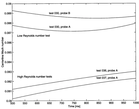
The Mach number history for low and high pressure tests is presented in Figure 2-9. For low pressure test 030, measurements from probe A and B agree to within 1% and the Mach number magnitude varies by less than 1% throughout the usable part of the test during

which the throttle plates are choked. For the high pressure tests, the Mach number increase with time by as much as 2%.

Under theoretical conditions, the Mach number should remain constant so long as the inlet guide vanes are choked. During a blowdown test, several factors can cause the Mach number to change slightly with time:

1. During a test, the inlet pressure and temperature decay, causing the Reynolds number1 to decrease by 10 to 15% in a 500 ms time span. Theoretically, the decrease in Reynolds number causes boundary layers to grow and the core flow Mach number to increase. The sensitivity of the Mach number to Reynolds number changes was evaluated by running a 2-D coupled viscous/inviscid model (UNSFLO, cf. Chapter 4) of the stage flow for conditions corresponding to t = 500 ms and t = 1000 ms and for the low and high pressure tests. The Mach number upstream of the NGV changed by less than 0.1% for both the high and low pressure cases. Although these figures are expected to underestimate the effects of Reynolds number change as the 2D model does not account for the endwall boundary layers, it can be concluded that Reynolds number effects play a minor role in the variation of core flow Mach number.

2. As the tunnel walls heat up to gas temperature, the boundary layer stabilizing effect of the cold wall vanishes [26]. The boundary layer thickness increases, enhancing the effect of increasing Reynolds number mentioned above. This factor is accounted for in the numerical simulation described above.

3. The recovery factor of the pressure probes changes with Reynolds number. However, this effect was found to be negligible from empirical testing by the Pitot static probe manufacturer.

4. The response of the Kulite pressure sensors is temperature dependent. Their mea-surement is expected to drift as they heat up to gas temperature.

5. The curvature of the Mach number trace might be an artifact of the curve fitting of the experimental data.

'The Reynolds number is defined as: Re = PtMD, where M is the local Mach number and D is the inner annulus diameter.

Test Pressure Reavg A A eA Aefc 030 32 psi 9.38 x 105 0.808 0.797 -036 104.5 psi 2.28 x 106 0.854 - -037 104.5 psi 2.25 x 10 0.859 - -038 94.7 psi 2.35 x 106 0.825 - -039 100.4 psi 2.37 x 10 0.856 - -040 104.5 psi 2.26 x 106 0.863 -

-Table 2.3: Ratio of the inferred effective area to the geometric area in the plane of the mass flow probe.

Mass Flow

l/Ae ff was computed from the mass flow probe data. Mass flow was also predicted by

Keogh [24] using Venturi nozzle measurements. Since Aeff is unknown, it was derived by taking the fraction of rhVenturi corrected by (rzh/Aeff)Mass flow probe. Figure 2-7 shows mass flow as predicted by the correction of the Venturi measurements and by the mass flow probes. The calculations agree to within 1% for the entire usable span of the data. The agreement between Probe A and B is better than 1% for the shape of the curve and 1% for the calculation of Aeff

Table 2.3 presents calculations of the effective area for different test conditions. The results agree with theoretical expectations: the effective area increases with Reynolds num-ber as boundary layers thin out when the flow becomes less viscous. Successive tests at the same test conditions yield effective areas agreeing to within less than 0.5%. The agreement can also be observed by comparing the corrected mass flow time history of tests with similar conditions (cf. Figure 2-10).

2.9

Chapter Summary

The concept of a dynamic pressure probe was presented, along with its applications to calculating Mach number and mass flow. Several conclusions and recommendations are available at this point of the instrument development.

1. It is possible to build a 1% accurate dynamic pressure probe and to use it to calculate mass flow with 1% uncertainty.

2. The oscillations generated by the start-up transient are a major limitation on the quality of the signal as their amplitude is of the same order as the differential pressure being measured. Further investigation in the origin of the oscillations would help to determine if the oscillations can be filtered out or if they have important physical relevance.

3. The 5 psi Kulite sensors used did not survive successive rounds of high pressure testing as the start-up transient generated differential pressures in excess of 15 psi, the burst pressure of the instrument. For subsequent high pressure tests, a more rugged sensor should be utilized.

4. The mass flow calculated using the mass flow probe data decayed at the same rate as the mass flow calculated using the corrected Venturi nozzle measurement. Hence, the theoretical correction derived by Keogh [24] correctly predicts the dynamics of the tunnel.

5. The original goal for this research was for the three probe combination to serve as a stand alone mass flow measuring device. In order to do so, a correlation of Reynolds number and effective area is necessary. This can be achieved using the Venturi nozzle measurements as a reference. Such a correlation should be compared with results from theoretical modeling of the inlet flow.

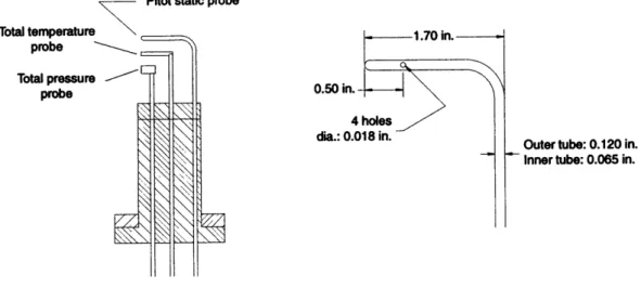
Pitot static probe

Total temperature probe

Total pressure

probe

Outer tube: 0.120 in. Inner tube: 0.065 in.

Figure 2-6: Schematic of the mass flow probe and dimensions of the Pitot tube.

1000

750 Time [ms]

Figure 2-7: Turbine mass flow as a function of time (Test 030).

0.50 in.

---4 holes dia.: 0.018 in.

1000

200 400 600

Time [ms]

(a) Total pressure probes

400 600

Time [ms]

(b) Dynamic pressure probes

8 I0

800 1000

(c) Total temperature probes

Figure 2-8: Mass flow probe pressure and temperature signals.

I, i i i i | i i i , Si Si 0.25 0.2 0.15 0.1 0.05 -''" 1000 n -4%. nrl .-/

0.09

0.089 test 030, probe B

0.088test

030, probe A 0.087

Low Reynolds number test E 0.086 CO S0.085 C 0.084 0.083 test 036, probe A

High Reynolds number tests test 037, probe A 0.082

0.081

0.08

500 550 600 650 700 750 800 850 900 950 1000

Time [ms]

Figure 2-9: Time history of Mach number for low and high Reynolds number tests.

x 10-7.4

7.3 test 030, probe B

7.2 - - _ test 030, probe A

7.1 Low Reynolds number test 7

Ca

E 6.9

6.8- test 039, probe A

High Reynolds number tests

test 037, probe A 6.7 6.6-6.5 500 550 600 650 700 750 800 850 900 950 1000 Time [ms]

CHAPTER

3

NON-INTRUSIVE STUDY OF TURBINE

FLOW: PARTICLE IMAGE

VELOCIMETRY

3.1

Introduction

In the last two decades, flow visualization techniques for unsteady flows have been con-stantly improved. Particle Image Velocimetry (PIV) is the latest method used in this field of research and generates instantaneous velocity fields by non-intrusive means. It has been tested extensively for the visualization of simple cases such as the flow around cylinders. It is only recently that the technique has been applied to more complex cases such as turbomachinery flows. Several research groups have reported PIV results in cascade exper-iments [18]. This chapter presents the results of one of the first attempts at applying PIV in fully scaled rotating turbomachinery .

The application of PIV to turbomachinery presents several challenges. First, installing the required instrumentation inside a turbine stage is a complex process. Second, the application of PIV to transonic flows is difficult because high accelerations are present in the flow and the experiment must be designed so that the seeding particles accurately follow the flow to capture these changes. The trade-offs involved are described below and 'To the best knowledge of the author, the only other successful applications of PIV in a rotating turbo-machinery stage were by Wernet in a transonic axial compressor [28] and by Bryanston-Cross in a transonic turbine stage [10].

are complemented with the results of the experiment.

3.2

Flow Visualization using Particle Image Velocimetry

The latest innovations in the field of experimental fluid flow visualization have been the suc-cessful applications of particle-image velocimetry to unsteady flows. This particle-imaging method belongs to a broader class of velocity-measuring techniques, known under the com-mon name of Pulsed Light Velocimetry (PLV). The author refers the reader to a review article by Adrian [3] for an excellent discussion of the subtleties of pulsed-light velocime-try and more specifically particle-image velocimevelocime-try. The following description is a brief introduction to the topic and should allow the reader to understand some of the issues and trade-offs present in the experimental application of PIV.

3.2.1 Pulsed-Light Velocimetry

The different techniques, grouped under the name of pulsed-light velocimetry, consist in tracking the displacement of discrete markers present in the flow. By monitoring the position of the markers over different, known, time intervals, the local velocity, V, of the marker can be calculated as:

(Y, t) a A(,t) (3.1)

At

where As' is the displacement of the marker located at F at time t, during the time interval

At separating successive observations of the markers.

The different PLV methods are characterized by the properties of the markers used. Solid particles in gases and liquids have been used as well as gaseous bubbles in liquids and liquid droplets in gases. On a smaller scale, molecules have also served as markers. In all cases however, PLV consists in repeatedly illuminating the flow and recording the image of the markers using an optical device.

3.2.2

Particle-Image Velocimetry

Particle-Image Velocimetry distinguishes itself from other PLV techniques in that the mark-ers are particles that are statistically always individually distinguishable. In other words, the density of the particles is small enough that the distance between them guarantees an individual image for each marker on the imaging medium.

Before going into the details of PIV image processing, it is useful to look at the technical implementation of the method. Although three dimensional PIV has been successfully demonstrated [21], this research will deal only with the two-dimensional application. The general principles of two-dimensional PIV are as follows: the flow to be studied is seeded with particles of appropriate properties (cf. Section 3.3.3); a light sheet is pulsed in the plane of interest; the illuminated particles scatter light back into an optical system oriented perpendicular to the sheet; the plane of focus of the optical system coincides with the plane of the light sheet and the image is recorded on a optical recording medium.

The two most popular recording medium are photographic film and digital camera imag-ing system. The digital system is more practical than the photographic film as its data can be transferred to a computer for automatic post-processing. However, digital imaging tech-nology is not advanced enough to be applied to all PIV applications. Three factors prevent this leap. First, digital cameras do not yet offer the same resolution as photographic film. A typical digital camera consists of an array of 1000 x 1000 pixels. The region of interest must therefore be small enough so that the particles correspond to at least the size of a pixel. Second, image files are very big and today's computer systems cannot always han-dle the rapid inflow of data necessary for high speed digital imaging. Finally, the frame acquisition speed must be fast, so that the particle displacement between successive frames can be assumed to be linear. For high speed flow applications, which require a very small

At between frames, the best digital cameras are still too slow and high speed photographic

cameras must be used.

Particle image velocimetry was differentiated above from other techniques of pulsed-light velocimetry by the low probability that separate particles will overlap on the image. Within this range of conditions lie two extremes, low-density PIV or Particle-Tracking Velocimetry

In particle-tracking velocimetry, the distance traveled by a particle between two succes-sive light pulses is small compared with the mean distance between adjacent particles. The velocity field is obtained by tracking the displacement of individual particles.

In high-density PIV, the density of particles is high enough that the displacement of individual particles between successive light flashes is larger than the mean distance between adjacent particles, but not so much that two particles overlap in the image. Tracking each particle would be time consuming due to their number and ambiguous due to the proximity of the particles. Instead of following individual markers, the displacement of small groups of particles is measured. The use of high-density PIV is tied to advanced image processing algorithms using cross-correlation or auto-correlation to track the displacement of the groups of markers. Adrian provides a detailed explanation of the procedure [3]. This method is a good complement to CFD: its output is a velocity field on a structured grid as opposed to a solution made up of randomly located velocity vectors for particle tracking velocimetry. The drawback, however, is that the scale of the observable flow phenomena is limited, as in CFD, by the size of the interrogation cells over which the correlation is executed.

The time interval between successive frames is an additional constraint in the application of PIV. In many engineering flows, the time interval necessary to calculate an approximately instantaneous velocity of the particles is small compared to the acquisition speed of the best digital imaging systems. In most turbomachinery applications, for example, the flow is transonic, and images corresponding to successive light flashes cannot be recorded on different frames. Instead, two or more images are superimposed on a single imaging medium. Although in theory this is not a problem for either of the high- or low-density methods, it brings about some ambiguities in the analysis. For example, it can be difficult to distinguish the particles of the first light flash from those of the second light flash. This can affect the accuracy of the solution. In particle-tracking velocimetry, the particles at different instants of times can be mistaken as being adjacent particles. The direction of velocity can also be ambiguous, as particles from successive instants in time can be identified in space but not in time. Adrian [3] explores several options to alleviate this problem, including using different colors of light pulses on color photographic paper.

In the experiment presented herein, photographic film was chosen as the imaging medium for double exposure low-density PIV. This decision was driven by two factors: (1) for