2D and 3D simulation of grain growth in olivine aggregates using a full field model based on the level set method

HAL Id: hal-01866105

https://hal-mines-paristech.archives-ouvertes.fr/hal-01866105

Submitted on 3 Sep 2018

HAL is a multi-disciplinary open access archive for the deposit and dissemination of sci-entific research documents, whether they are pub-lished or not. The documents may come from

L’archive ouverte pluridisciplinaire HAL, est destinée au dépôt et à la diffusion de documents scientifiques de niveau recherche, publiés ou non, émanant des établissements d’enseignement et de

2D and 3D simulation of grain growth in olivine

aggregates using a full field model based on the level set

method

Jean Furstoss, Marc Bernacki, Clément Ganino, Carole Petit, Daniel

Pino-Muñoz

To cite this version:

Jean Furstoss, Marc Bernacki, Clément Ganino, Carole Petit, Daniel Pino-Muñoz. 2D and 3D simula-tion of grain growth in olivine aggregates using a full field model based on the level set method. Physics of the Earth and Planetary Interiors, Elsevier, 2018, 283, pp.98-109. �10.1016/j.pepi.2018.08.004�. �hal-01866105�

2D and 3D simulation of grain growth in olivine

aggregates using a full field model based on the level set

method

Jean Furstoss1, 2*, Marc Bernacki2, Cl´ement Ganino1, Carole Petit1, Daniel Pino-Mu˜noz2

1_{Universit´e Nice Cˆote d’Azur, CNRS, OCA, IRD, G´eoazur, France}

2_{MINES ParisTech, PSL Research University, CEMEF-Centre de mise en forme des}

mat´eriaux, CNRS UMR 7635, France *Contact: furstoss@geoazur.unice.fr

Abstract

In this study, we investigate grain growth within pure olivine systems through numerical simulations. The level set (LS) approach within a finite element (FE) context enables modeling 3D microstructural evolutions such as grain growth. As this phenomenon is inherently a 3D mechanism, the comparison between 2D and 3D models shows differences despite the use of 2D/3D trans-formation tools. The 2D level set approach is then compared with 2D models of grain growth performed with the ELLE software 1_{. Both approaches give} consistent results. Our results confirm the rapid annealing of fine grained structures in pure olivine aggregates at temperatures of 1473 and 1573K. Comparison with previously published experimental results yields an esti-mate of the activation energy at 171−180 kJ·mol-1_{for olivine grain boundary} mobility.

Keywords: Grain growth kinetics, olivine, full field modeling, level set, 2D-3D comparison

1. Introduction

Microstructures are parts of the memory of rocks and the knowledge of thermal and/or mechanical loading that led to their formation can be used to predict their future behaviour.

Indeed, it is well known that rheological properties of rocks (and in general of crystalline materials) are closely related to their microstructures, because the latter influences dominant creep mechanisms. For example, strain localiza-tion in ductile mantle shear-zones may be controlled by lithospheric mantle microstructures inherited from prior deformations [1]. In fact, it has been shown that lithospheric mantle weak zones primarily control tectonic pro-cess such as strain localization at plate boundaries [2]. The microstructure involves a variety of parameters (grain size, distribution of mineral phases, lattice orientations, etc.). As a result, several mechanisms potentially able to weaken mantle rocks have been suggested including grain size reduction [1], phase transformations [3], and the development of lattice preferred orienta-tion [4]. Even if the combined role of these mechanisms in the weakening is likely, the well known association of ductile shear zones with grain size reduction suggests this process is one of the most important [5].

In naturally deformed mantle rocks, a switch from grain size insensitive (GSI) to grain size sensitive (GSS) creep can occur by decreasing grain size below a certain critical size depending on several conditions (e.g. stress, strain rate, temperature) [5]. Theoretically in GSS creep regimes, the strain rate is

re-lated to the inverse of grain size [6]. Experiments show that olivine rocks weaken considerably with decreasing grain size [7] initiating or enhancing strain localization at zones of low grain size. After localization priming, a positive feedback between strain weakening and strain localization (by the coexistence of grain reduction and GSS creep) permits the development of permanent weak plate boundaries [1, 8].

Dormant plate boundaries (defined as long lived lithospheric weak zones at geological time scale) are interpreted to be ancient deformation zones (such as suture zones). By considering the decrease of grain size as the most rel-evant mechanism of rock weakening, the superposition of dormant plates boundaries with zones where deformation has involved dynamic recrystal-lization (and reduced peridotite grain size) can be explained [1]. Geological record evidences that over period of about 250 Myr, a full orogenic cycle can take place, reactivating dormant plate boundaries [9], which means that grain size still remains small enough and enables deformation by GSS creep. Grain growth kinetics in peridotites (and especially in olivine) has already been explored by experimental [10, 11, 12] and numerical [13, 14] approaches. It has been shown that mantle lithospheric temperatures (i.e. 900-1600 K) may allow efficient grain growth, which would result in a rapid erasing of fine-grained weak zones. In this paper, we study the grain boundary migra-tion (GBM) and its effect for microstructure evolumigra-tions within a pure olivine system using numerical simulations.

A large variety of methods can be used to compute numerical microstruc-ture evolution, including grain growth. They can be divided in two main

categories :

• mean field models, which describe microstructure evolution through homogenized system characteristics (e.g. mean grain size, grain size distribution, mean stored energy, Smith-Zener limit grain size).

• Full field models, which describe the system topology and simulate its evolution.

Mean field models can be based either on phenomenological observations, or on theoretical (such as thermodynamical) considerations, or both. More re-cently, in the metallurgy community, some mean field models obtained from full field simulations have been proposed [15]. Even if these models enable large scale computations with low computational cost, their predictions are only suitable in the range determined by the corresponding experiments, or in combination with full field models, which will help to calibrate them. An-other drawback is related to their limitation to predict local phenomena such as abnormal grain-growth.

Several full field modeling techniques have been developed in order to sim-ulate microstructure evolutions in rocks. Hereafter a simple classification of these methods is proposed.

- Stochastic methods such as Monte Carlo Potts model [13] consist of voxel-based grain shape description, where each lattice site in a grain is given the same ”spin”, and microstructure evolution is computed according to the probability for a site to change its spin. Although these methods have high scalability and low computational costs, a precise calculation of the mean cur-vature calculation needed to model grain growth is not straightforward with

a voxelized microstructure. Another issue inherent to Monte Carlo methods is to perform accurate scaling between the Monte Carlo step and the physical time step. Furthermore, capturing different physical mechanisms through the same numerical scheme tends to be extremely complicated since it is difficult to accurately control the change probability change for each mechanism. - Front-tracking methods [16] are deterministic approaches and are based on the explicit description of interfaces. In 2D, grain boundaries are de-scribed by nodes connected by segments and the microstructure evolution is computed by applying evolution equations to either nodes or segments. Ad-vantages of tracking methods are the ease of computing interface properties (such as mean curvature, normal) and reasonable numerical cost. However, topological events such as grain shrinkage are difficult to manage from a nu-merical point of view, and become really problematic in 3D. Moreover, intra-granular fields, such as stored energy gradient, cannot be described without the use of a secondary mesh describing the grain interiors. Nonetheless the front-tracking approach is well suited for modeling grain growth. A front tracking method is implemented within the microstructural modeling plat-form ELLE [17] (https://www.elle.ws), a now classical tool for modeling rock microstructural evolution in the state of the art.

- Finally, grain growth can also be modelled by using an implicit description of interfaces, which is done either in the phase field method [18], or in the level set method [19], and permits to avoid the tracking of interfaces and the issue of handling topological events. The latter is the one chosen for this work. The numerical approach presented in [20, 21, 22, 19] is used to describe microstructural evolutions of materials (essentially metals) during

industrial processes. This approach deals with a LS description of interfaces in a FE formulation.

One of the aims of the present work is to give a review of the existing full field modeling techniques developed in order to compute microstructural evolution of rocks at the mesoscale (i.e. grain-scale). In this context, we will focus on the grain growth phenomenon which will be initially analyzed in a physical point of view. Then, different numerical implementation techniques of the GBM mechanism will be presented.

We also test, in 2D and 3D, the adaptability of the LS formulation for non-metal materials such as pure olivine system considering only the grain growth mechanism without deformation. The 2D results will be compared with those obtained within the ELLE’s software. Our results also bring reflex-ion elements in the geological context of perennial weak zones preservatreflex-ion described above.

2. The grain growth phenomenon and its numerical modelisation

2.1. Grain boundary migration

Grain growth occurs in polycrystalline materials by grain boundaries mi-gration (GBM) through the microstructure leading to the reduction of Gibbs free energy. Driving forces for GBM can derivate from different factors as capillarity, difference of stored energy (by lattice defects) between grains or solid-solid phase transformations, in the case of multiphase material [16]. Generally the velocity (~v) of a boundary can be expressed as [23] :

~

where M is the grain boundary mobility, F the driving force per unit area and ~n the outward unit vector normal to the grain boundary.

By considering a monophasic polycrystal system where only the reduction of interface energy (capillarity) is taken into account (corresponding to a static or normal grain growth), the grain boundaries move to minimize the surface energy and the driving force is generally approximated as :

F ~n = −γκ~n, (2)

where γ and κ are respectively the grain boundary energy and the mean curvature of the grain boundary. It is important to notice the dependence of the mean curvature definition with the number of dimensions considered. Indeed, the 3D curvature is a diagonalizable tensor where the non-zero eigen-values are called the main curvatures. Thus the 3D mean curvature is defined as the trace of this tensor, i.e. the sum of the main curvatures.

When the grain boundary mobility and energy are assumed isotropic and uniform throughout the domain, the developed microstructure can reach a foam-like structure where boundaries are smoothly curved and triple junc-tions form 120◦ inter-boundary angles. In this context of ideal grain growth, the kinetics is expected to follow an inverse power-law, describing the increase of the mean grain size as a function of time.

2.2. Microdynamics simulation for grain growth : a review

Many programs have been developed in Earth Sciences to simulate mi-crodynamic processes (e.g. grain growth, Smith-Zener pinning) by full field modeling [13, 16, 14] (i.e. by considering topological description of the

mi-crostructure). There is presently one general platform called ELLE [17] (web-site : https://www.elle.ws) that gather the modeling of several mechanisms such as grain growth or crystallisation from a melt. This software, which has the advantage of being open source and subject to ongoing development by a large community of researchers, bonds a variety of physical process simulation methods making it a very multipurpose code. Moreover the soft-ware package includes a set of codes for individual processes which can be combined within the same simulation. In this section, we review numerical approaches that can be used in microstructural evolution modeling. We will focus on the Earth Science field, although many of these methods are widely used in other research fields (e.g., metallurgy).

2.2.1. Voxel-based methods

Within the Monte Carlo (MC) and cellular automata (CA) approaches, the microstructure is usually discretized using a regular lattice by a set of volume elements called voxels. Each voxel represents a group of atoms and is characterized for instance by an orientation (or a spin) indicating which voxels belong to a grain (figure 1.a).

The microstructure typically evolves by changing the state of the vox-els, applying different methods depending on the approach. While MC ap-proaches are stochastic, using probabilistic laws to change the state of a voxel, CA can be based on either stochastic or deterministic rules which modify the state of each CA cell. MC and CA models have benefited from considerable efforts from the research community over the last decades and are actually relevant despite several complications inherent to this group of methods.

(a) (b)

(c) (d)

Figure 1: (a) example of a voxelized 2D triple junction, a grain is represented by a set of voxel containing the same spin value, (b) a triple junction discretized using vertex (e.g. ELLE approach), (c) an interface between two grains represented by the order parameters of the phase field approach, (d) an interface between two grains represented by level set functions.

the effective grain boundary energy. This energy is usually given by a sum of pairwise voxel interactions which can be expressed in a monophasic and isotropic case by [24] :

Eboundtot = 1 2γa N X i=1 z X j=1 Kij, (3)

where a is a constant with a unit of length, N is the total number of lattice sites, z the number of nearest neighbors of the voxel i and Kij is the kernel which controls the strength of the pairwise interactions. The kernel is usually constant for voxels within a given neighborhood Ni of the ith voxel such as :

Kij =    1 − δqiqj if j ∈ Ni 0 otherwise, (4)

where qi and qj are the spins of the lattices i and j and δ is the Kroneker delta. However, this kernel can be enriched by functions taking into account, for instance, the distance between the voxels [25]. Eq.3 can suffice to compute the microstructure evolution driven by the reduction of total boundary en-ergy, but the grain boundary curvature is not consider here. In order to take into account this driving force, CA and MC models can calculate the mean curvature of a boundary by different methods. The explicit computation (generally used in CA models) is often done by variations of the template method [29] which consists of determining the portion of volume enclosed by a template that lies on one side of the interface. The mean curvature of the opposite side is then approximated by a linear function of the computed volume. Implicit calculation can also be used (rather for MC models) by con-necting the energy change accompanying the change of a voxel spin and the mean curvature of the grain boundary. In all cases, the total energy of the system is computed and can be used by transition rules governing the spin change of voxels, stochastic for MC methods (such as the Metropolis

func-tion) and generally deterministic for CA models (such as rule arising from the grain boundary motion eq.1). All the voxels (or a set of voxels around boundaries) are selected (randomly within MC methods) and may switch to the state of one of all adjacent voxels according to the transition rules. The time increment is then realized after applying the transition rules to a single voxel or to all voxels for respectively MC and CA methods. The determina-tion of the incremented time varies with each methods and guaranteeing a physical meaning is not straightforward.

The voxel-based methods such as MC and CA methods are very flexible and have demonstrated their capabilities to simulate microstructural evolu-tions [13]. The use of voxel and regular grids is convenient for parallel com-putations with low computational costs. Intragranular fields such as stored energy gradient can be easily taken into account but the discretization of a microstructure with regular lattice of voxels can influence the evolution of the system and may be unable to accurately reproduce the curved surfaces. This regular lattice may also be limiting for the modeling of large deformations, which require adaptative remeshing procedures as in many other numerical approaches. Moreover, in MC methods it is difficult to relate model units with physical ones, especially for the time unit (which is usually expressed in monte carlo time steps). MC simulations parameters are then calibrated based on the comparison between numerical and experimental results [26, 27]. The CA approaches generally deal with transition rules, which avoid the is-sue of the units of length physical meaning and permit an easier comparison with experimental systems [28].

2.2.2. Front-tracking methods

Front tracking models represent grain boundaries by a network of polyhe-dral area in 3D, formed by lines and connected nodes (figure 1.b). In contrast to vertex methods [30], this network forms a real mesh, defining connectiv-ity between nodes and permitting a FE resolution. Thus the microstructure evolves through the movements of the nodes according to physical laws. This approach permits to describe a 3D polycrystal by a 2D mesh (and a 2D case by a 1D mesh) and therefore limits the computational cost.

There are various approaches to compute the GBM in a front-tracking context depending on the resolution technique used to move the nodes de-scribing the microstructure.

The first consists on the sequential displacement of the nodes (i.e. one node at a time), within these approaches the polyhedral network does not need to be a real mesh (e.g. no connectivity of the nodes needed) and the methods are more relevant to the vertex methods. An expression describing the GBM is applied to the different nodes of the system one by one. These expressions can derivate, for instance, from a driving force of the GBM such as eq.2. The approach implemented in the ELLE software to compute the GBM [16], use the free energy gradient as :

dE(r)

dr = −F, (5)

where E(r) is the free energy field over the position r and F is the driving force of GBM. The moving direction of a node is then determined as the direction producing the maximum reduction of free energy. Hereafter the magnitude of the velocity v of the node is computed taking into account

the implications of the node sequential displacements and the node is moved with a magnitude of v∆t with ∆t the time increment.

Another way to compute the evolution of the nodes is the use of a FE res-olution scheme [31]. Within this context, the main aim is to transform the equations governing the motion of a grain boundary (such as eq.2) in a sys-tem of 3N (in 3D) ordinary differential equations (ODEs) with N the number of nodes on the interfaces. The resolution of the linear system leads to the displacement of all the nodes, and to the evolution of the microstructure.

The tracking of boundaries permits to access easily the interface prop-erties such as mean curvature. Moreover, nodes can have a number of at-tributes (e.g. interfacial energy, grain boundary mobility) that allow to define the properties of the interface they represent. However, topological events such as shrinkage or nucleation of grain are difficult to manage in terms of remeshing, especially in 3D. Another disadvantage with this approach is that grain interiors are not described by the mesh, which may be problematic to take into account some properties at the grain scale such as intragranular stored energy or intragranular nucleation.

2.2.3. Phase field methods

The phase field methods (PFMs) provide a powerful methodology to de-scribe phase transformations and were initially used to model crystallization or sub-solidus phase transformations. Actually, the PFM are also used in or-der to simulate microstructural evolutions such as recrystallization and grain growth [18]. Within the PFMs, the description of the interfaces is implicit, and the microstructure is described by continuous functions of the spatial

coordinates and time also called order parameters. Within each grain only one of these parameters take the value of unity and the others have a zero value. Across the grain boundaries the phase field parameter continuously varies from 1 to 0 by usually following an hyperbolic trigonometric function of the Euclidean distance to the interface (figure 1.c). The microstructure evolves through the change of order parameters by resolving a given set of coupled partial differential equations.

The phase field approach considers that grains and grain boundaries are related to the free energy F of the system. This free energy can be expressed as an integral of the free energy density over the all domain, taken into ac-count all the order parameters describing the microstructure, and the gradi-ent energy coefficigradi-ent which controls the boundary thickness. The calculation of the free energy density introduces also phenomenological parameters, as the gradient energy coefficient which has to be calibrated on experimental data or chosen arbitrarily. The microstructure evolution is then a result of the minimization of this free energy F through the resolution of the time-dependent Ginzburg-Landau equations :

∂ηi(r, t)

∂t = −L diF

dηi(r, t), i = 1, ..., p, (6) where di

d denotes a functional derivation, ηi, i = 1, ..., p are the order param-eters, r and t are respectively the spatial and time variables and the kinetic coefficient L is related to the grain boundary mobility. This set of equation can be discretized and then solved for instance by a FE or finite volume method.

the microstructural evolutions of a polycrystal. Nevertheless, the formal-ism introduces numerical parameters, such as the gradient energy coefficient (related to the boundary thickness), which are not straightforward to fix and largely impact the simulation results. Finally, PFMs have relatively high computational costs and the parallelization of codes are often needed to compute the evolutions of representative systems, which is quite common for all numerical methods dealing with microstructure evolution in context of a FE strategy.

3. Level set approach for grain growth

The level set framework used here for the full field modeling of the mi-crostructure supports implicit description of grain boundaries by level set functions in a FE framework. Initially designed for metallurgic considera-tions, as microstructure evolutions in industrial processes, this model has already been used in 2D or 3D to simulate dynamic [20] or static [32] re-crystallization and grain growth [19, 22] with possible inert second phase particles [33] in some metallic materials. As for the phase field approach, the main weakness of this procedure is its computational cost, related to the large number of LS functions needed to describe the microstructure. One of the aims of the present work is to test the adaptability of this formulation to a geological material such as olivine aggregates considering only grain growth.

3.1. The level set formalism

A LS function ψ is defined over a domain Ω as the signed distance function to the interface Γ of a sub-domain G of Ω [21] (figure 1.d). The formulation

adopted here involves that values of ψ are calculated at each node of the mesh and the sign convention states ψ > 0 inside G and ψ < 0 elsewhere :

∀t    ψ(X, t) = ±d(X, Γ(t)),X ∈ Ω Γ(t) = {X ∈ Ω, ψ(X, t) = 0} (7)

where X represents space variables. Therefore the outwards normal ~ni and the mean curvature κi of the grain constituting ψi are defined by :

~ ni(X, t) = −−−→∇ψi(X, t) kψi(X, t)k , (8) κi(X, t) = ~∇. ~ni(X, t). (9)

κi is then equivalent to the opposite of the laplacian of the LS function if ψi remains a distance function (i.e. kψi(X, t)k = 1) at least in a thin layer around the interface. Restoring the metric property (redistancing) of LS functions is an inherent problem of LS methods and reinitialization algorithms must be used during the simulation in order to keep LS functions as signed distance functions. The reinitialization algorithm implemented in the used formalism is based on a direct method (exact analytic reconstruction of the distance function) enhanced by a k-d tree space partitioning technique [34] for each LS function at each timestep.

The microstructure evolution governed by the velocity field defined in eq.1 can be therefore computed by solving a set of NG (number of grain within the system) diffusive equations :

∀i ∈ {1, .., NG}    ∂ψi(X ,t) ∂t − γM ∆ψi(X, t) = 0 ψi(X, t = 0) = ψi0(X) (10)

Nevertheless, the approach described above requires as much LS functions as grains and the numerical cost of the resolution of eq.10 and reinitializa-tion becomes quickly problematic. In order to reduce the computareinitializa-tion time, Global level set (GLS) functions are used to achieve steps previously men-tioned [21]. These GLS functions do not represent only one grain but several grains separated from each other by a certain number of grains. In order to avoid numerical coalescence during the evolution of the microstructure, if grains represented by the same GLS function are becoming too close from each other they can be transferred to another GLS function by a grain recol-oring algorithm [21]. Thus the number of functions needed to represent the microstructure is much smaller than the number of grains constituting the system, which significantly reduces the computational cost of the simulation. Another point must be highlighted considering the LS method : the diffusive formulation (i.e. eq.10) can lead to vacuums and overlaps apparitions after each time step. To address this issue, a simple treatment is performed on each GLS function after solving diffusive equations presented above [35]:

ψi(X, t) = 1

2(ψi(X, t) − maxi6=j(ψj(X, t)) (11)

Applied on a multiple junction this treatment allows to removing the vacuum (or overlap) [35].

3.2. Initial microstructure & boundary conditions

To simulate microdynamics processes as grain growth, an initial mi-crostructure is needed and can be generated either by an algorithm or by dig-italizing experimental data as optical microscope images for example. Here, in order to respect a given grain size distribution, the considered digital mi-crostructures are generated with a Vorono¨ı-Laguerre Dense Sphere Packing (VLDSP) algorithm [36] based on the dropping and rolling method, which enables to generate a polycrystal in agreement with the required grain size distribution if the domain size is large enough.

Boundary conditions are also needed to solve partial differential equations as eq.10 in a FE scheme. Boundary conditions used here (null Neumann bound-ary condition) imposed orthogonality between grain boundaries and domain boundaries. This imposed angle does not lie with any physical consideration and may induce some errors due to boundary effects if the number of grain in the domain is not large enough. A convergence study of the mean grain size evolution in terms of domain size was then automatically considered in order to ensure convergence of the results while limiting the calculation domain size and so the numerical cost. It must be highlighted that periodic bound-ary conditions (optimal for minimizing the calculation domain size) are not considered in our numerical framework in order to be able to consider local remeshing during calculations as described in the following section.

3.3. Mesh refinement and timestep

A grain growth simulation as described above does not need a fine mesh in grain interiors but the grain boundary surroundings need to be finely de-scribed. A mesh refinement around the interfaces is used in 2D in the FE

context, and this refinement is adapted during the simulation in order to follow the grain boundary movements [37]. Local remeshing during 3D cal-culations was not performed, as it does not represent any gain in terms of time calculation, oppositely to the 2D context where local adaptive remesh-ing strategy is interestremesh-ing in terms of numerical cost [15]. Thus in 3D, a initial mesh is chosen fine enough to describe grain boundaries based on a convergence study on the mean grain size evolution as a function of the initial homogeneous finite element size. The FE mesh does not evolve during the simulation.

The choice of the incremental time is another crucial point : it must be large enough to limit the computational time but small enough to describe accu-rately the grain size evolution, even if an implicit FE resolution is used here. The solution employed here in 2D and 3D use an adaptative timestep ∆t which is computed at each step as follows :

∆t = cEp vm

(12)

where c is a percentage of the refined mesh thickness Ep (typically 15%) in 2D and vm is the maximum value of the grain boundary velocity over the all domain computed with eq.1 and 2. In 3D the product cEp is replaced by percentage of the cell size. This approach enables to have at any time an optimized timestep which can be long if the microstructure evolves slowly, and short if the GBM is fast.

4. Methods

4.1. Initial grain size distribution and grain boundary mobility and energy Physical parameters needed for investigating grain growth are the mo-bility and the energy of grain boundaries. These parameters are anisotropic in natural rocks [38] and this anisotropy can be evaluated experimentally or numerically by various methods [39]. However the introduction of an anisotropy of the interfacial energy changes the FE formulation of the prob-lem which is a work in progress. Even if some basic anisotropic laws such as a Read-Shockley can already been treated [40] they will not be presented. In this paper, we made the assumption of isotropic grain boundary properties. Indeed, in pure olivine aggregates, anisotropic grain evolution mainly occurs as a result of uneven distribution of dislocation densities and crystalline pre-ferred orientation due to rock deformation [41], which is not considered here. The grain boundary energy used here has been established by Duyster & St¨ockhert [38] for high angle grain boundaries of olivine in natural peridotite and yields a value of 1.4 J·m-2.

The grain boundary mobility (m4_·J-1_·s-1_{) is a temperature dependent} param-eter which is usually defined with an Arrhenius law :

M = M0e−Q/RT, (13)

where M is the mobility, M0 the reference mobility, Q the activation en-ergy, R the gas constant and T (K) the absolute temperature. In order to determine M0 and Q, experimental procedures monitor the mean grain size

evolution of a rock sample during an isothermal annealing treatment at dif-ferent temperatures. In this paper, for the firsts simulations the values of M0 and Q will be based on those determined by Karato [10] i.e., respectively, 4.104 mm4·J-1_·s-1 _{and 160 to 200 kJ·mol}-1 _{depending on experimental} condi-tions. Then, the comparison between the simulation and the experimental results enable to adjust the material parameters M0 and Q (see section 5.1). In order to compare experiments and simulations, similar initial grain size distributions must be used. Figure 2 represents the experimental initial dis-tribution in volume fraction and the log-normal law used to approximate this distribution.

Figure 2: Blue squares : initial grain size distribution as volume fraction from Karato 1989 [10], yellow line : best fitting log-normal law imposed in our VLDSP algorithm

a log-normal distribution characterized by a mean grain size µ = 2.24 µm, a standard deviation σ = 0.82 µm and so a σ/µ ratio of 0.37.

4.2. Tracking grain growth kinetics

Considering the three main following hypotheses :

• the grain boundary mean curvature κ can be approximated by 1

R where R is the equivalent radius of the grain,

• the mobility and the grain boundary energy are isotropic and uniform, • the temperature is constant,

the Burke and Turnbull (1952) model can be built from eq.1 and allows describing grain growth kinetics only through the average grain size as [42]:

< R >2 − < R0 >2= 1

2M γt, (14)

where R and R0 correspond respectively to average grain radii at times t and 0 s.

Even if this model does not take into account neither topological nor neigh-boring effects, it has been used in some experimental cases, as for example to determine first order mobility knowing the grain boundary energy [10, 43]. In these experiments, a sample is annealed at constant pressure and temper-ature and an average grain size is measured at different times. This process applied at different temperatures allows determining the reference mobility M0 and the activation energy Q in the Arrhenius law of the mobility (eq.13). However, real microstructures do not always satisfy the hypothesis used in this model. Eq.14 is then often generalized according to [19] :

< R >2 − < R0 >2= αM γtn (15)

where α and n are dependent on initial grain size distribution [19], grain shape or presence of secondary phases, pores or melt [11]. In the case of a monophasic system without pores or melt, values of α and n can be plotted, for log-normal distributions, against the σ

µ ratio [19, 22]. As an example, α and n are respectively close to 1₂ and 1 (leading to eq.14) for initial grain size distributions which are log-normal with a σ

µratio equal to 0.45 considering 2D grain growth [19] and may be equal to 0.35 considering 3D grain growth [22].

4.3. Determining grain sizes

The initial grain size distribution of Karato [10] presented in fig.2 comes from the olivine powder which served to build the sample. This distribution has been measured by an Elzon Particle Counter which indicates that this distribution is a 3D distribution. However, during the annealing experiment, the mean grain size distribution has been monitored by 2D observations of a thin section of the sample. In the numerical simulations presented here we seek to be coherent with this experimental procedure (tab.1).

For 2D grain growth simulations (LS2 and V2), we use the initial grain size distribution of Karato 1989 [10] transformed by the inverse Salykov analy-sis [44] which gives a volume distribution with a mean grain size of 2.05 µm, a standard deviation of 0.68 µm and so a σ/µ ratio of 0.33. This analysis permits to compute a statistical equivalent 2D distribution from a 3D one. Then we compare computed grain sizes during the annealing treatment with

Table 1: Characteristics of the different simulations realized within the present work.

the ones obtained by Karato.

For the 3D grain growth simulations (LS3/3 and LS3/2), the initial grain size distribution used is the one presented in fig.2. Then, for the determination of the grain size evolution during the annealing treatment and the comparison with the experimental ones, two cases will be distinguished. First, the com-puted 3D grain size distributions will be transformed by the inverse Saltykov analysis (LS3/3) in order to get 2D equivalent distribution comparable with experimental observations. Second, we estimate the 2D grain sizes by pro-jecting the LS functions on regularly spaced slices cross cutting the domain volume. We then compare experimental data with average grain sizes com-puted from these 2D slices. The initial grain size distributions, in number, for all the simulations are presented in fig.3.

The LS3/2 grain size distribution has more small grains than the LS3/3 one. This has already been noticed [45, 46] and may be attributed to the effect of the left distribution truncation.

Figure 3: Initial grain size distributions for the different simulations (see tab.1). As explained in the section the LS3/3 distribution is a 2D Saltykov analysis on 3D grain size distribution and the LS3/2 distribution is obtained by averaging the distributions of the ten 2D sections.

4.4. Computational domain size and boundary influence

During the annealing simulations, the number of grains decreases and the portion of grain boundaries in contact with the computational domain boundaries increases. The evolution of these grain boundaries is dictated by the imposed boundary conditions (see section 3.2) and does not have any physical meaning. Thus when the grain number in the domain is not large enough, the grain growth mechanism is polluted by boundary effects and the mean grain size evolution diverges from the Burke and Turnbull model. In order to have a representative number of grains over a duration comparable with the experimental data (few hours), a larger domain must be considered. Square computational domains of increasing sizes have been tested (see fig.4) in order to determine the optimal domain size, with the best ratio of grain

number versus computational cost.

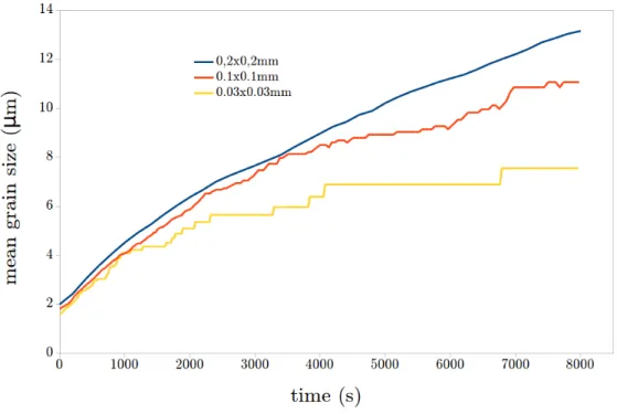
Figure 4: Mean grain size evolution during annealing 2D simulation at 1573 K, for a mobility activation energy of 200 kJ and for square computational domains of 0.2x0.2, 0.1x0.1 and 0.03x0.03 mm initially containing respectively 3700, 960 and 110 grains.

The apparition of steps on the evolution curves reflects the fact that the num-ber of grains is no longer representative. Indeed, these steps appear earlier for smaller domains with lower initial grain number. After the convergence study of the mean grain size evolution with the calculation domaine size, we choose for this study squared or cubic domains with size of 0.2x0.2mm and 0.15x0.15x0.15mm in 2D and 3D, respectively.

Concerning the slices of the LS3/2 simulation (see tab.1), in order to get a representative number of grains, we do not consider the results obtained

when the number of grains per slice is lower than 200.

4.5. ELLE grain growth simulations

Within the ELLE software, two algorithms are available to simulate the evolution of a microstructure through grain growth driven by capillarity. These two algorithms are based on the front-tracking method described in the section 2.2.2.

The first one, called ”growth” uses normalized material parameters and phys-ical units. In fact, the simulation results of this algorithm are neither de-pendent on the grain boundary mobility/energy nor on the temperature, timestep or unit of length values. The only parameters which have an impact on the simulation are the numerical parameters such as the switch distance, which controls the maximal displacement of a node during a timestep. Even if the obtained microstructures have similar topological aspect than those ob-tained from an experimental annealing (such as those obob-tained by Karato [10] : i.e. foam texture), the grain growth kinetics cannot be considered within a physical point of view.

The second one, called ”gbm” takes into account the material parameters and the physical units in the calculation of the node displacements. In this case, grain growth kinetics from ELLE simulation can be compared with those obtained with experimental data. Thus the V2 simulation (see tab.1) is performed by using the ”gbm” algorithm.

The ELLE’s microstructure is initialized by using the ”ppm2elle” utility which transform a ppm image into a ELLE file. The image used is the one obtained initially by the LS2 (see tab.1) 2D level set simulation.

5. Results

We first present the calibration of the grain boundary mobility activation energy with the experimental data for the different simulations (see tab.1). Then, the grain size distributions at different time steps are compared for the different simulations. Finally, one of the computed microstructures is compared with the experiment and we present an annealing simulation of a more complex microstructure with an initially heterogeneous grain size distribution.

5.1. Material parameters calibration

For all the simulations described in section 4.3 and in order to deter-mine the best-fitting activation energy we adopt the following approach : the interfacial energy and the reference mobility are fixed respectively at 1.4 J·m-2 _{and 4.10}4 _mm4_·J-1_·s-1_{, then an activation energy is chosen. Here we} select an initial intermediate value of 180 kJ·mol-1_{between those determined} experimentally by Karato 1989 [10]. A grain growth simulation is then per-formed until reaching a < R >2 _{− < R}

0 >2 value equal to one of those obtained experimentally. Using eq.14 and the Arrhenius law of the mobility, the expression of the optimized activation energy Q can be expressed as :

Q(J.mol−1) = 180.103− RT ln(tsimu texp

) (16)

where tsimu and texp are respectively the simulation time and the experimen-tal time needed to reach the same < R >2 − < R0 >2 value. By using the

experimental results of Karato 1989 [10] and averaging the obtained values with the different points at 1473K and 1573K, we obtain a best-fitting ac-tivation energy value. For both the LS3/3 and LS3/2 simulations, the best fitting activation energy value is 171.5 kJ·mol-1 while the LS2 and V2 ones lead to 185 kJ·mol-1_{. However, the kinetics obtained with those values are} quite different between the 3D (LS3/3 and LS3/2) and the 2D simulations (LS2 and V2) in particular at the beginning where the 2D grain growth is slower than the 3D one and at the end where the 2D grain growth is faster than the 3D one. The reference mobility and the activation energy for the LS2 and V2 simulations are then adjusted. The assumed activation energy is lowered (180 kJ·mol-1_{), and the reference mobility is adjusted to fit the} LS3/3 grain growth kinetics. Final mobility parameters (M0(mm4·J-1·s-1), Q(kJ·mol-1_{)) for the different simulations are (4.10}4_{, 171.5)}LS3/3,LS3/2 _and (6.104, 180)LS2,V 2.

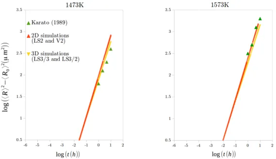
Figure 5 shows the experimental grain growth kinetics from [10] and the computed and then extrapolated (using the Burke and Turnbull mean field model, eq.15) grain growth kinetic for the 3D simulations (LS3/3 and LS3/2) and the 2D ones (LS2 and V2). Those results are presented through the plot of log(< R >2 _{− < R}

0 >2) against log(t) which allows to determine n and α of the eq.15 mean field model by fitting the obtained results.

For both the LS3/3 and the LS3/2 simulations the grain growth kinetics are similar (fig.5 and fig.6) and the n and α values are respectively equal to 0.88 and 1.27. For the LS2 and V2, the grain growth kinetics are also almost the same with n = 0.93 and α = 1.34. Those adjusted parameters are not far from those obtained for these initial distributions with the mean field models

Figure 5: Mean grain size time evolution at 1473 K (left) and 1573 K (right), M0 =

4.104 _mm4_·J-1_·s-1 _{and Q = 171.5 kJ·mol}-1 _{for the LS3/3 and the LS3/2 simulations and}

M0= 6.104mm4·J-1·s-1 and Q = 185 kJ·mol-1for the LS2 and the V2 ones. The

experi-mental results of Karato [10] are plotted in green.

of Cruz-Fabianno et al. [19] for 2D grain growth and Maire et al. [22] for 3D grain growth.

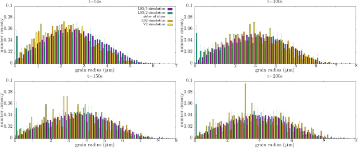
All simulation results at 1573K are plotted on fig.6, for their own best-fitting mobility parameters. The related distributions are presented in fig.7 at different time steps. Within this figures, the maximum time for the com-parison is limited by the LS3/2 simulation in which the number of grains per slice decreases rapidly under 200.

Figures 6 and 7 show that the different simulations (2D or 3D, LS or V) give consistent results. The mean grain size evolutions (fig.6) are close to each other. Even if the LS3/2 simulation underestimates the mean grain size

Figure 6: Evolution of the mean grain size for each simulations : LS3/3 (yellow), LS3/2 (orange) and standard deviation as error bars, LS2 (green), V2 (brown)

Figure 7: Comparison of the grain size distributions for the different simulations during an annealing treatment at 1573K.

in comparison with the LS3/3 one, the mean grain size of the latter is within the standard deviation of the one determined by the slices averaging. The grain size distribution evolutions (fig.7) also show consistent results. The LS3/2 still includes more small grains than the other ones, which may be explained by the reasons exposed in section 4.3.

5.2. The olivine grain growth kinetics

Once the material parameters are calibrated (through the activation en-ergy in our case), the computed grain growth kinetics is in good agreement with the experimental one (see fig.5). Moreover, the grain dimension and geometry obtained from the computed 2D microstructure after 2 hours of annealing is comparable to the one presented by Karato 1989 (fig.8) [10].

Figure 8: Left : experimental microstructure from [10] after 2 hours annealing at 1573K, right : LS2 simulation after 2 hours annealing at 1573K

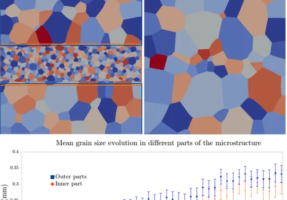
In order to simulate a system more similar to a natural deformed rock, we consider a fine grained zone (mylonitic or ultramylonitic texture) embedded

in a zone of coarser grains (porphyric texture) (fig.9), representing a fine-grained shear band.

The microstructure is considered as homogeneous when the mean grain sizes of the inner part and the outer parts, plus or minus the standard devia-tion, are equal. At 1250K, the time needed to erase the scar does not exceed 200 days (fig.9).

6. Discussions

The capillarity-driven GBM is a 3D physical mechanism controlled at the first order by the boundary curvatures. In fact, the 2-dimensional as-pect of the curvature can strongly impact the grain growth kinetics. For instance, a highly curved boundary in one direction may be submitted to a null driving force if the curvature in the other direction is also elevated with an opposite sign. Although X-ray CT scanning is increasingly used to measure 3D fabrics in rocks [47], the technique would be of limited interest for a monomineralic aggregate. Therefore, interpretations of 2D observa-tions have to be taken with caution, keeping in mind the 3D character of the observed mechanism. Thus, numerical simulations are convenient tools to study this 2D/3D paradigm, which is mostly ignored in the state-of-the-art grain growth experiments.

Our results suggests that, as grain growth is inherently a 3D process, it should be modelled also in 3D. However, the numerical costs of a 3D sim-ulation may be quickly prohibitive. The Saltykov method is an interesting alternative to the use of 3D model since it allows determining an equivalent

3D grain size distribution (or inversely). Hereafter, 3D numerical simulations and their 2D equivalent can be realized in order to define some transition laws for instance to adjust a 3D mean field model from a 2D one.

The comparison of the 2D LS simulation with the ELLE simulation shows very good agreement. Nevertheless the ELLE grain growth simulation has a much lower computational cost than the LS one : one hour is enough to simulate the evolution of the system in the first case while the same LS com-putation takes a few dozen hours. Indeed, as mentioned above, the ELLE approach only discretises the interfaces, which is equivalent to deal with a 1D mesh while the LS calculation needs a 2D mesh. Moreover, within the ELLE simulation, the displacement of the nodes is sequential while the LS approach uses a FE resolution which is more expensive in computational resources. Nevertheless, the ELLE approach can become limited for some applications. First, the non description of grain interiors may limit the sim-ulation of some processes for instance those which depend on intragranular stored energy. The LS approach permits to describe intragranular fields within a same framework which can be useful for instance for dynamic re-crystallization modeling. Second, the 3D implementation within a vertex approach is not straightforward and uncommon in the state of the art, due to the difficulty of managing topological events as shrinking or nucleation of grains. As the grain growth process is inherently a 3D mechanism, it can be useful to model it in 3D, that is something the LS approach allows to do.

Considering the GBM in a pure olivine system and based on our re-sults, we conclude that a surface energy of 1.4 J·m-2 _{and a mobility of}

M0 = 4.104 mm4·J-1·s-1, Q = 171.5 kJ·mol-1 for 3D simulation and M0 = 6.104 mm4·J-1_·s-1_{, Q = 180 kJ·mol}-1 _{for 2D ones, are satisfying estimates} for olivine/olivine grain boundaries. The distribution evolutions presented in fig.7 are close to each other. This shows that 2D simulations can predict equivalent distributions of 3D simulations by adapting the (M0, Q) couple. In all cases, 2D or 3D observations of a 3D system or 2D computations, the grain growth kinetics is extremely rapid compared to the typical geological timescale, the grain size increasing from a few micrometers to a few tenths of millimeters in a dozen hours. Within the context of the dormant plate boundaries, it signifies the rapid erasing of fine-grained weak zones.

If we consider that the presence of multiple fine-grained bands as in fig.9 is responsible for the existence of weak zones, the erasing scar time can be evaluated as the time needed to homogenize the microstructure. Our results show this time which is extremely fast against the hundreds Myr for the persistence of natural weak zones. As mentioned previously, the fast grain growth kinetics and so the rapid scar erasing can be attributed to the pu-rity of the systems considered here. Indeed, both the experimental samples of Karato [10] and the numerical microstructures of the present work are only composed of olivine. The inhibition of grain growth in dormant weak zone conditions (i.e. non-deformed), can be explained by the presence of secondary phases (SP) in mantle rocks.

The presence of SP in peridotites such as pyroxenes, spinels, plagioclase and garnets will influence different physico-chemical processes. Indeed, depend-ing on second phase particles (SPP) size and nature, a drag pressure can act on grain boundaries and counteract grain growth driving pressure [48]

(well known as Smith-Zener pinning mechanism [49]). The presence of free surfaces and pores may also act as SPP and impede the GBM through the Smith-Zener pinning mechanism [50, 33]. The movement of interfaces be-tween two phases may also be limited because of the kinetics of chemical elements transfer throughout the interface [12]. In our simulations, the grain boundaries move to minimize their total surface without be impeded by any SPP or interphase boundaries. As the natural peridotites also contain a certain amount of second phases, it seems obvious that the time needed to erase inherited structures in natural rocks is much larger than in pure olivine aggregates [1].

7. Conclusion

The simulations performed within the present work highlight the 3D char-acter of the grain growth mechanism, and the influence of the mode of obser-vation of grain size evolution during a grain growth experiment or simulation. As 3D simulations or experimental observations are not always easy to set up, 2D ones are often used to determine 2D effective material parameters which are different from the physical 3D ones in the presented results. Those effective parameters allow to predict a 2D behavior equivalent to a 3D one. A phenomenological law which evaluates the physical material parameters M γ from the ones calibrated with 2D observations may be determined either by the realization of similar simulations with different grain size distributions or by experiments coupling 3D and 2D observations during annealing.

Like in previous papers focusing on grain growth in pure olivine aggre-gates [10, 11], we observe that grain growth kinetics is very fast. In fact,

this grain growth rate suggests that persistent weak zones should disappear within a few hundred days which is not observed in nature. Thus, pure olivine aggregates are not relevant to study the persistence of weak zones at the geological time scale through the grain growth in mantle rocks. Nev-ertheless, neither the grain boundary pinning by SPP, nor the influence of interphase boundaries have been considered in this work. In future work, the numerical simulation will be enriched in order to take into account those different mechanisms. The simulations presented in this work have permitted to determine M γ products for the olivine/olivine grain boundaries which can be used within more complex simulations.

8. Acknowledgements

We thank all the members of the ELLE development group, in particular Lynn Evans for her help with ELLE grain growth simulations.

This work was supported by CNRS INSU 2018-programme TelluS-SYSTER. The supports of the French Agence Nationale de la Recherche (ANR), ArcelorMittal, AREVA, ASCOMETAL, AUBERT&DUVAL, CEA, SAFRAN through the DIGIMU Industrial Chair and consortium are grate-fully acknowledged. The authors thank Editor Key Hirose and two anony-mous reviewers for their constructive comments.

9. References

[1] Bercovici, D., Ricard, Y., 2012. Mechanisms for the generation of plate tectonics by two-phase grain-damage and pinning. Physics of the Earth and Planetary Interiors, 202-203:27–55.

[2] Heron, P.J., Pysklywec, R.N., Stephenson, R., 2016. Lasting mantle scars lead to perennial plate tectonics. Nature Communications, 7:11834.

[3] Tingle, T.N., Green, H.W., Scholz, C.H., Koczynski, T.A., 1993. The rheology of faults triggered by the olivine-spinel transformation in Mg₂GeO4 and its implications for the mechanism of deep-focus earth-quakes. Journal of Structural Geology, 15:1249–1256.

[4] Tommasi, A., Knoll, M., Vauchez, A., Signorelli, J.W., Thoraval, C., Log´e, R., 2009. Structural reactivation in plate tectonics controlled by olivine crystal anisotropy. Nature Geoscience, 2:423–427.

[5] Platt, J.P., Behr, W.M., 2011. Grainsize evolution in ductile shear zones: Implications for strain localization and the strength of the lithosphere. Journal of Structural Geology, 33:537–550.

[6] Kohlstedt, D., 2007. Properties of rocks and minerals - constitutive equations, rheological behavior, and viscosity of rocks. Treatise on Geo-physics, 2:389–417.

[7] Vissers, R.L.M., Drury, M.R., Hoogerduijn Strating, E.H., Spiers, C.J., van der Wal, D., 1995. Mantle shear zones and their effect on lithosphere strength during continental breakup. Tectonophysics, 249:155–171.

[8] Gueydan, F., Pr´ecigout, J., Mont´esi, L. G. J., 2014. Strain weakening enables continental plate tectonics. Tectonophysics, 631:189–196.

[9] Wilson, T., 1966. Did the Atlantic close and then re-open ? Nature, 211:676–681.

[10] Karato, S., 1989. Grain growth kinetics in olivine aggregates. Tectono-physics, 168:255–273.

[11] Evans, B., Renner, J., Hirth, G., 2001. A few remarks on the kinetics of static grain growth in rocks. Int J Earth Sciences (Geol Rundsch), 90:83–103.

[12] Hiraga, T., Tachibana, C., Ohashi, N., Sano, S., 2010. Grain growth systematics for forsterite ± enstatite aggregates: Effect of lithology on grain size in the upper mantle. Earth and Planetary Science Letters, 291:10–20.

[13] Solomatov, V.S., El-Khozondar, R., Tikare, V., 2002. Grain size in the lower mantle: constraints from numerical modeling of grain growth in two-phase systems. Physics of the Earth and Planetary Interiors, 129:265–282.

[14] Jessell, M.W., Kostenko, O., Jamtveit, B., 2003. The preservation po-tential of microstructures during static grain growth. J. metamorphic Geol., 21:481–491.

[15] Maire, L., Scholtes, B., Moussa, C., Bozzolo, N., Pino-Mu˜noz, D., Set-tefrati, A., Bernacki, M., 2017. Modeling of dynamic and post-dynamic recrystallization by coupling a full field approach to phenomenological laws Materials and Design, 133:498–519.

[16] Becker, J.K., Bons, P.D., Jessel, M.W., 2008. A new front-tracking method to model anisotropic grain and phase boundary motion in rocks. Computers & Geosciences, 34:201–212.

[17] Bons, P.D., Koehn, D., Jessel, M.W., 2008. Microdynamics simulation. Lecture notes in earth sciences, 106.

[18] Chen, L.Q., Yang, W., 1994. Computer simulation of the domain dy-namics of a quenched system with a large number of nonconserved order parameters: The grain-growth kinetics. Physical Review B, 50(21):15752–15756.

[19] Cruz-Fabiano, A.L., Log´e, R., Bernacki, M., 2014. Assessment of sim-plified 2D grain growth models from numerical experiments based on a level set framework. Computational Materials Science, 92:305–312.

[20] Bernacki, M., Resk, H., Coupez, T., Log´e, R.E., 2009. Finite element model of primary recrystallization in polycrystalline aggregates using a level set framework. modeling and Simulation in Materials Science and Engineering, 17:064006.

[21] Scholtes, B., Shakoor, M., Settefrati, A., Bouchard, P.O., Bozzolo, N., Bernacki, M., 2015. New finite element developments for full field mod-eling of microstructural evolutions using the level set method. Compu-tational Materials Science, 109:388–398.

[22] Maire, L., Scholtes, B., Moussa, C., Bozzolo, N., Pino-Mu˜noz, D., Bernacki, M., 2016. Improvement of 3D mean field models for capillarity-driven grain growth based on full field simulations. J Mater Sci, 51(24):10970–10981.

[23] Rollett, A., Humphreys, F., Rohrer, G.S., Hatherly, M., 2004. Recrys-tallization and Related Annealing Phenomena : Second Edition.

[24] Mason, J.K., 2015. Grain boundary energy and curvature in Monte Carlo and cellular automata simulations of grain boundary motion. Acta materialia, 94:162–171.

[25] Mason, J.K., Lind, J., Li, S.F., Reed, B.W., Kumar, M., 2015. Ki-netics and anisotropy of the Monte Carlo model of grain growth. Acta Materialia, 82:155–166.

[26] Hallberg, H., 2011. Approaches to Modeling of Recrystallization. Metals, 1(1):16–48.

[27] Rollett, A.D., 1997. Overview of modeling and simulation of recrystal-lization. Progress in materials science, 42(1-4):79–99.

[28] Miodownik, M.A., 2002. A review of microstructural computer models used to simulate grain growth and recrystallisation in aluminium alloys. Journal of Light Metals, 2(3):125–135.

[29] Bullard, J.W., Garboczi, E.J., Carter, W.C., Fuller Jr., E.R., 1995. Numerical methods for computing interfacial mean curvature. Compu-tational Materials Science, 4:103–116.

[30] Weygand, D., Brechet, Y., Lepinoux, J., 2001. A Vertex Simulation of Grain Growth in 2D and 3D. Advanced Engineering Materials, 3(1-2):67–71.

[31] Kuprat, A., George, D., Straub, G., Demirel, M.C., 2003. Modeling microstructure evolution in three dimensions with Grain3D and LaGriT. Computational Materials Science, 28:199–208.

[32] Scholtes, B., Boulais-Sinou, R., Settefrati, A., Pino-Mu˜noz, D., Poitrault, I., Montouchet, A., Bozzolo, N., Bernacki, M., 2016. 3D level set modeling of static recrystallization considering stored energy fields. Computational Materials Science, 122:57–71.

[33] Agnoli, A., Bozzolo, N., Log´e, R., Franchet, J.M., Laigo, J., Bernacki, M., 2014. Development of a level set methodology to simulate grain growth in the presence of real secondary phase particles and stored en-ergy - Application to a nickel-base superalloy. Computational Materials Science, 89:233–241.

[34] Shakoor, M., Scholtes, B., Bouchard, P.O., Bernacki, M., 2015. An efficient and parallel level set reinitialization method - Application to micromechanics and microstructural evolutions. Applied Mathematical modeling, 39:7291–7302.

[35] Merriman, B., Bence, J.K., Osher, S.J., 1994. Motion of multiple junc-tions : A level set approach. Journal of Computational Physics, 112:334– 363.

[36] Hitti, K., Bernacki, M., 2013. Optimized Dropping and Rolling (ODR) method for packing of poly-disperse spheres. Applied Mathematical mod-eling, 37:5715–5722.

[37] Resk, H., Delannay, L., Bernacki, M., Coupez, T., Log´e, R., 2009. Adap-tive mesh refinement and automatic remeshing in crystal plasticity finite element simulations. modeling Simul. Mater. Sci. Eng., 17(7):075012.

[38] Duyster, J., St¨ockhert, B., 2001. Grain boundary energies in olivine derived from natural microstructures. Contrib Mineral Petrol, 140:567– 576.

[39] Rohrer, G.S., 2011. Grain boundary anisotropy : a review. Journal of Materials Science, 46:5881-5895. DOI:10.1007/s10853-011-5677-3

[40] Fausty, J., Bernacki, M., Pino-Mu˜noz, D., Bozzolo, N., 2018. A new level set finite element formulation for anisotropic grain growth. ECCM-ECFD 2018 conference, Glasgow, UK, June 11-15 2018

[41] Boneh, Y., Wallis, D., Hansen, L.N., Krawczynski, M.J., Skemer, P., 2017. Oriented grain growth and modication of frozen anisotropy in the lithospheric mantle. Earth and Planetary Science Letters, 474:368–374.

[42] Burke, J.E., Turnbull, D., 1952. Recrystallization and grain growth. Progress in Metal Physics, 3:220–244.

[43] Hirth, G., Kohlstedt, D.L., 1995. Experimental constraints on the dy-namics of the partially molten upper mantle : Deformation in the diffu-sion creep regime. J. Geophys Res, 100:1981–2001.

[44] Saltykov, S.A., 1958. Stereometric Metallography. Metallurgizdat, Moscow.

[45] Tarquini, S., Armienti, P., 2003. Quick determination of crystal size distributions of rocks by means of a color scanner. Image Anal Stereol, 22:27–34

[46] Weygand, D. , Brechet, Y. and Lepinoux, J., 2001. A Vertex Simulation of Grain Growth in 2D and 3D. Adv. Eng. Mater., 3:67–71.

[47] Bedford, J., Fusseis, F., Lecl`ere, H., Wheeler, J., Faulkner, D., 2017. A 4D view on the evolution of metamorphic dehydration reactions Scien-tific Reports, 7:6881. DOI:10.1038/s41598-017-0716

[48] Herwegh, M., Linckens, J., Ebert, A., Berger, A., Brodhag, S.H., 2011. The role of second phases for controlling microstrctural evolution in polymineralic rocks: A review. Journal of Strctural Geology, 33:1728– 1750.

[49] Smith, C.S., 1948. Grains, phases, and interphases: an interpolation of microstructure. Transactions of the American Institute of Mining and Metallurgical Engineers, 175:15–51.

[50] Scholtes, B., Ilin, D., Settefrati, A., Bozzolo N., Agnoli, A., Bernacki, M., 2016. Full field modeling of the Zener pinning phenomenon in a level set framework - discussion of classical limiting mean grain size equation. Superalloys 2016: Proceedings of the 13th International Symposium on Superalloys, 497–503.

Figure 9: Left top: initial microstructure with fine grain zone representative of a shear band, the domain size 3x3mm, right top : microstructure after 185 days annealing at 1250K, bottom : grain size evolutions of the inner part (orange) and the outer parts (blue) of the microstructure, the color are also relative to the colored boxes of the left top picture, the error bars are related to the standard deviation of calculated mean grain size. The grain colors are related to the index of the global level set (GLS) function which describes the considered grain.