HAL Id: hal-00749234
https://hal.archives-ouvertes.fr/hal-00749234
Submitted on 7 Nov 2012
HAL is a multi-disciplinary open access
archive for the deposit and dissemination of
sci-entific research documents, whether they are
pub-lished or not. The documents may come from
teaching and research institutions in France or
abroad, or from public or private research centers.
L’archive ouverte pluridisciplinaire HAL, est
destinée au dépôt et à la diffusion de documents
scientifiques de niveau recherche, publiés ou non,
émanant des établissements d’enseignement et de
recherche français ou étrangers, des laboratoires
publics ou privés.
Atlantic in the 1980s and 2000s.
Elodie Martinez, David Antoine, Fabrizio d’Ortenzio, Clément de Boyer
Montégut
To cite this version:
Elodie Martinez, David Antoine, Fabrizio d’Ortenzio, Clément de Boyer Montégut. Phytoplankton
spring and fall blooms in the North Atlantic in the 1980s and 2000s.. Journal of Geophysical Research.
Oceans, Wiley-Blackwell, 2011, 116, pp.C11029. �10.1029/2010JC006836�. �hal-00749234�
Phytoplankton spring and fall blooms in the North Atlantic
in the 1980s and 2000s
Elodie Martinez,
1David Antoine,
1Fabrizio D
’Ortenzio,
1and C. de Boyer Montégut
2Received 24 November 2010; revised 5 September 2011; accepted 7 September 2011; published 19 November 2011.
[1]
Phytoplankton chlorophyll
‐a (Chl) seasonal cycles of the North Atlantic are described
using satellite ocean color observations covering the 1980s and the 2000s. The study
region is where warmer SST and higher Chl in the 2000s as compared to the 1980s have
been reported. It covers latitudes from 30°N
–50°N and longitudes from 60°W–0°W,
where two phytoplankton blooms take place: a spring bloom that follows stratification of
upper layers, and a fall bloom due to nutrient entrainment through deepening of the
mixed layer. In the 1980s, spring and fall blooms were of similar amplitude over the
entire study region. In the 2000s, the fall bloom was weaker in the eastern Atlantic (east
of 40°W), because of a delayed deepening of the mixed layer at the end of summer
(mixed layer depth (MLD) determined from in situ data). Conversely, the spring bloom
of the eastern Atlantic was stronger in the 2000s than it was in the 1980s, because of a
deeper MLD and stronger winds in winter. In the Northwestern Atlantic (northwest of
38°N
–40°W), little differences are observed for spring and fall blooms, and for the
wintertime MLD. Our results show that the links between upper layer stratification, SST
changes, and biological responses are more complex than the simple paradigm that
sequentially relates higher stratification with warmer SST and an enhanced (weakened)
growth of the phytoplankton population in the subpolar (subtropical) region.
Citation: Martinez, E., D. Antoine, F. D’Ortenzio, and C. de Boyer Montégut (2011), Phytoplankton spring and fall blooms in the North Atlantic in the 1980s and 2000s, J. Geophys. Res., 116, C11029, doi:10.1029/2010JC006836.
1.
Introduction
[2] Phytoplankton growth results from the conjunction of
nutrient supply and light availability. When both demands are satisfied, phytoplankton can experience rapid growth, leading to large biomass accumulations in the upper layers generally referred to a phytoplankton bloom. This phe-nomenon is important for regional to global carbon budgets, and also drives bottom‐up processes throughout the pelagic food chain [Richardson and Schoeman, 2004]. There are at least two types of phytoplankton blooms that arise from different combinations of physical forcing: spring and fall blooms.
[3] The onset of a spring bloom occurs when upper layer
stratification is sufficient for phytoplankton to use the nutrients previously brought to the surface by deep winter mixing [Sverdrup, 1953]. This is also the time when surface irradiance increases toward the summer solstice maximum. Spring blooms end when surface waters are nutrient depleted due to consumption by phytoplankton (bottom‐up control), and also because of zooplankton grazing (top‐ down control) [Banse, 1992].
[4] A fall bloom is conversely driven by the deepening of
the surface mixed layer at the end of summer, leading to nutrient entrainment in the surface layer. It is also controlled by a reduction in grazing pressure due to the seasonal ver-tical migration of mesozooplankton toward deep waters [Colebrook, 1982]. It is dissipated (diluted) by mixing and energy starved by declining light in fall‐winter [Longhurst, 1995].
[5] Phytoplankton spring blooms in the North Atlantic are
the most pronounced of any open ocean region [Yoder et al., 1993; Kennelly et al., 2000]. They have been the focus of many studies [Colebrook, 1979; Ducklow and Harris, 1993; Siegel et al., 2002]. Mechanisms of their rise were first described 60 years ago [Sverdrup, 1953], and are still being investigated [i.e., Dutkiewicz et al., 2001; Siegel et al., 2002; Follows and Dutkiewicz, 2001; Lévy et al., 2005; Ueyama and Monger, 2005; Behrenfeld, 2010]. Fall blooms have been reported in the North Atlantic Drift Region (NADR; 43°N–56°N; 43°W–0°W) [Colebrook, 1982; Longhurst, 1995; Dandonneau et al., 2004; Lévy et al., 2005].
[6] The aim of our study is to investigate differences in
the North Atlantic (30°N–50°N and 60°W–0°W) phyto-plankton blooms in spring and fall between 1979–1983 and 1998–2002. These two time periods are, respectively, the first 5 years of the Coastal Zone Color Scanner (CZCS, NASA ocean color mission launched in 1978 [Hovis et al., 1980]) and Sea‐viewing Wide Field‐of‐view Sensor (Sea-WiFS, NASA mission launched in 1997; [McClain et al., 1
Laboratoire d’Océanographie de Villefranche, UMR 7093, CNRS, UPMC, Université de Paris, Villefranche‐sur‐Mer, France.
2
Laboratoire d’Océanographie Spatiale, IFREMER, Plouzane, France. Copyright 2011 by the American Geophysical Union.
2004]) satellite ocean color missions (see below for justi-fication of using only subsets of these two time series). The surface chlorophyll‐a concentration (Chl) derived from these satellite observations is used as a proxy for phyto-plankton biomass.
[7] Sea surface temperature (SST) can be used as an
indicator of the ocean stratification, which is one forcing of phytoplankton variability [Behrenfeld et al., 2006]. How-ever, contradictory relationships between SST and Chl have been reported, which suggests that SST might be an ambiguous indicator of stratification. An inverse relationship between Chl and SST has been reported over about 60% of the global ocean using remote sensing [Behrenfeld et al., 2006; Martinez et al., 2009]. This inverse relationship is usually expected in nutrient‐limited subtropical regions, because a warming‐induced stratification would reduce the upward nutrient supply and then productivity [Sarmiento et al., 2004; Doney, 2006; Polovina et al., 2008]. Stratifi-cation would conversely increase productivity in subpolar gyres, which are light limited because of intense vertical mixing [Polovina et al., 1995; Doney, 2006]. A parallel relationship between Chl and SST is conversely observed over∼40% of the global ocean. This was shown, for instance, in the North Atlantic from the 1980s to the 2000s [Martinez et al., 2009], and related to a regime shift of the Atlantic Multidecadal Oscillation (AMO) from a cold to a warm phase in the mid‐1980s.
[8] Our aim here is to study the connection between
stratification and seasonal Chl cycles (blooms). Therefore, we investigate variability of Chl along with that of the mixed layer depth (MLD) and of the wind stress, which is a driver of the MLD. The corresponding data sets are pre-sented in section 2. In section 3, the spatial and seasonal variability of Chl and MLD are quantified using empirical orthogonal function (EOF) analyses. Then, their interannual variability within each of the two time periods is presented separately for the eastern and northwestern Atlantic, which differ both in terms of their physical and biogeochemical environments. The possible role of changes in wind stress intensity in generating the differences in MLD observed between the CZCS and SeaWiFS era is also examined. Results are summarized and discussed in section 4.
2.
Data
[9] Ocean color time series are provided by the CZCS
(November 1978–June 1986) and SeaWiFS (September 1997–December 2010) missions. Caution is necessary when comparing data from these two time series separated by an 11 year gap. We accordingly used the reprocessed data set generated by Antoine et al. [2005], who applied the same algorithms and an adapted calibration to both CZCS and SeaWiFS observations, providing two fully compatible 5 year time series. The years 1979–1983 were selected for the CZCS because there is virtually no data in 1984, and because the calibration became uncertain for the years 1985 and 1986. The reprocessed SeaWiFS data set was generated in 2003. Therefore, it only includes preceding years; i.e., the 5 years from 1998–2002. For the sake of simplicity, these two time periods will be referred to as the “CZCS period” and the“SeaWiFS period,” though they do not correspond to the full lifetime of these satellite missions. In order to
avoid repetition, they will be also occasionally referred to as “the 1980s” and “the 2000s,” although they do not include all years from each of these 2 decades. Embracing the full 13 year SeaWiFS time series would entail using the NASA standard data set, losing compatibility with the reprocessed CZCS data set and introducing essentially unknown uncer-tainty in the comparison. The archive used here is made of monthly composites with an 18 km resolution. It excludes shallow waters (depth < 200 m). Readers are referred to Antoine et al. [2005] for further understanding of how this reprocessing made the two data sets comparable.
[10] The database of in situ vertical temperature profiles
put together by de Boyer Montégut et al. [2004] allowed them to build a global monthly MLD time series starting in 1941. They determined MLD using a temperature criterion, as being the depth where the temperature is 0.2°C different from the temperature at 10 m. This reference depth was shown to be sufficiently deep to avoid aliasing by the diurnal temperature signal [de Boyer Montégut et al., 2004]. Here we extracted the North Atlantic (30°N–50°N and 60°W–0°W) monthly MLD over 1979–1983 and 1998– 2002. The number of observations is quasi‐identical over the two time periods (34,391 versus 32,444 observations, respectively). Their spatial distribution are similar and differ only over the area 40°N–50°N and 40°W–30°W, with slightly less data in 1979–1983 (not shown).
[11] Surface wind stress is one forcing of the interannual
MLD variability. We used the International Comprehensive Ocean‐Atmosphere Data Set (ICOADS), which provides gridded monthly summary products extending from 1800 onward, based on an extensive collection of surface marine data. We used the 1° enhanced product extracted monthly over 1979–1983 and 1998–2002, and derived the wind stress amplitude from its zonal and meridional components [Woodruff et al., 2010].
[12] Chl, MLD, and wind stress monthly fields were
averaged on a 2° by 2° grid and interpolations were carried out to fill empty grid cells. Linear interpolations in time were first performed in each cell, and only when the gap was of 1 month. Spatial interpolation along the longitude and latitude axes was subsequently performed only for single isolated empty cells. The MLD and wind stress data sets were barely impacted by this processing because their initial coverage was almost full. At the end, all 2° by 2° cells in the study region were filled with MLD and wind stress data, and 90% were filled with Chl data.
[13] In order to quantify the seasonal variability of Chl,
MLD, and wind stress in the North Atlantic over 1979–1983 and 1998–2002, Empirical Orthogonal Function analyses (EOFs) have been performed on anomaly fields. The first set of EOFs (section 3.2) was performed on Chl and MLD data to investigate their seasonal variability, and the anomaly fields were obtained by subtracting the average annual value in each 2° by 2° cell determined over 10 years; i.e., the 5 years of CZCS plus the 5 years of SeaWiFS. The second set of EOFs (section 3.3) was performed on MLD and wind stress data to highlight their interannual variability. The anomaly fields were therefore derived by subtracting the average monthly values determined over the 10 years.
[14] The potential implication on primary production of
the observed differences in Chl seasonal cycles has been evaluated using a wavelength‐, depth‐, and time‐resolved
light photosynthesis model [Morel, 1991; Antoine and Morel, 1996]. In addition to Chl, SST, and MLD, this model needs surface photosynthetically available radiation (PAR), which has been computed for clear‐sky conditions from date and latitude [Gregg and Carder, 1990] and cor-rected for cloudiness using a monthly cloud climatology. This climatology was derived from averaging ISCCP‐D2 monthly mean cloud data between July 1983 (the start of the ISCCP data set) and June 2006 [Rossow and Schiffer, 1999; http:// isccp.giss.nasa.gov]. Therefore, possible differences in cloudiness between the 1980s and 2000s are ignored, which means that differences in the modeled primary production are
due only to differences in Chl, SST, and MLD. It is worth noting that such a light photosynthesis model does not explicitly include the effect of nutrient limitation. It is a diagnostic model that uses the observed Chl as the indicator of the trophic state.
3.
Results
3.1. Basin‐Scale Spatial Features and Seasonal Cycles [15] The distributions of Chl and of the maximum MLD
(computed over 1998–2002) are displayed in Figure 1 for the purpose of illustrating the main features of the study region (30°N–50°N; 60°W–0°W), which includes the sub-tropical and subpolar phytoplankton regimes. For the pur-pose of facilitating the reading of the figures, the Chl value of 0.6 mg m−3is arbitrarily used to delineate regions of high Chl. This threshold corresponds to the green‐to‐yellow transition on color plates.
[16] At subpolar latitudes the annual phytoplankton
bio-mass cycle is dominated by the spring bloom, which occurs in response to increases in mean irradiance of the mixed layer. At lower latitudes in the subtropics, the biomass peak occurs during winter when mixing by winds and thermal convection replenish the euphotic zone with nutrients. This biomass peak is much reduced in comparison to high‐lati-tude spring blooms [Yoder et al., 1993]. The study region also encompasses five of Longhurst’s [1995] biogeochem-ical provinces. In the north, high Chl values appears in the North Western Continental Shelves (NWCS) province in the west and in the North Atlantic Drift (NADR) province in the east. These two provinces belong to the subpolar gyre (Figure 1a). In the south, low Chl values appear in the western and eastern North Atlantic Subtropical (NAST) provinces of the oligotrophic subtropical gyre. In the western region, the Gulf Stream (GFST) province separates the NWCS and NAST provinces. These biogeochemical province boundaries are partly driven by the oceanic dynamics [Longhurst, 1995]. Therefore, they also appear on the spatial distribution of the winter MLD maximum (MLDmax; Figure 1b). Northwest of 40°N–40°W in the
NWCS region, MLDmax is shallow and the cold Labrador
Current flows from the north. The southern boundary of the NWCS region is the Gulf Stream, which flows north-eastward and spreads in the northeastern region into the North Atlantic Current, where MLDmaxis deep (>∼150 m).
Further south, the Azores Current flows eastward then southeastward and MLDmax is about 100 m.
[17] The characteristics of the spring and fall blooms are
separately analyzed. The fall bloom refers to a Chl peak between September and January, and the spring bloom to a peak between February and August. These two time inter-vals cover the full year when taken together. The average and standard deviation of the Chl and MLD seasonal cycles over the entire study region are shown in Figure 2. In the subpolar region (from 40°N to 50°N and 60°W to 0°W; i.e., the NWCS and NADR provinces), the Chl seasonal cycle during the period 1979–1983 exhibited a fall bloom (Figure 2a, first peak of the thick dashed line) slightly stronger than the spring bloom (second peak, in May). In 1998–2002, the fall bloom was weaker and the spring bloom was dominant (Figure 2a, thick solid line). This dominant spring bloom was preceded by a maximum of Figure 1. (a) Average Chl and (b) maximum of MLD, both
calculated over the 1998–2002 period in the North Atlantic. The black box on both maps delineates the region of our study. The black line inside the box delineates the north-western region where the maximum MLD is shallower than 120 m, and which is referred in the text as the northwestern Atlantic region or the North Western Costal Zone. The bio-geochemical provinces are indicated in Figure 1a: the North Western Continental Shelves (NWCS), the North Atlantic Drift (NADR), the Gulf Stream (GFST), and the western and eastern North Atlantic Subtropical (NAST(W) and NAST(E), respectively) provinces. The surface currents are indicated in Figure 1b: The Labrador Current (LC), the Gulf Stream (GS), the North Atlantic Current (NAC), and the Azores Current (AC).
MLD that was deeper during the SeaWiFS era than it was during the CZCS era (Figure 2a, dashed versus solid thin lines).
[18] The average spring and fall distributions of Chl and
MLD for the two time periods are shown in Figure 3. These distributions show that the large fall bloom compared to the spring bloom during the CZCS era (Figure 2) was mainly located in the NADR rather than in the NWCS province (Figures 3a and 3c). The weaker fall bloom and stronger spring bloom in the 2000s are particularly evident in the NADR province (Figures 3b and 3d compared to Figures 3a and 3c). Finally, deeper wintertime MLD are mostly located in the GFST and NADR regions (Figures 3e and 3f). 3.2. Chl and MLD Interannual Variability in 1979–1983 and 1998–2002
[19] The results of EOF analyses performed on Chl and
MLD anomalies are shown in Figures 4 and 5. The two first EOFs modes of Chl seasonal anomalies respectively repre-sent 34% and 17% of the total variance (Figure 4). The spatial function of the first mode (Figure 4a) shows the strongest Chl seasonal variability in the transition zone, between the subpolar (NWCS and NADR) and subtropical (NAST) regions. The second mode (Figure 4b) highlights the highest Chl variability in the NADR province. The associated time functions (Figure 4c) show a spring bloom occurring earlier in the transition zone (red line, white background) than in the subpolar region (black line, white background). The spring bloom is initiated in the transition zone by the supply of nutrients from winter mixing, while further north in the subpolar gyre, where the ecosystem is likely to be light limited, the bloom occurs later when the
MLD becomes shallower than the critical depth [Sverdrup, 1953; Siegel et al., 2002].
[20] Conversely, the fall bloom occurred earlier in the
subpolar region (black line, gray background) than in the transition zone (red line, gray background). The fall bloom is initiated in the subpolar gyre when the mixed layer dee-pens at the end of summer and is progressively refueled with nitrate. Further south, a longer time is necessary for the deepening of the MLD to reach the nutrients that are deeper than northward.
[21] Besides these regional differences, the two time
functions show that fall booms were weaker and spring blooms were stronger in the 2000s than they were in the 1980s (Figure 4c). This pattern is emphasized in the tran-sition zone, where the fall bloom barely appeared in the 2000s (Figure 4c, small peaks in the 2000s as compared to the 1980s).
[22] The first mode of the EOFs performed on MLD
explains 76% of the total variance (only 3.8% for the second mode, not shown). The spatial distribution of the MLD variability mimics that of the annual MLDmax (Figure 1b). The strongest seasonal variability appears in the NADR region where the North Atlantic Current flows (Figure 5a). In the NAST(E), NWCS, and Labrador current regions, the MLD seasonal variability is weak and the MLDmax is
shallower than in the NADR region. The MLDmax occurs
around February–March (EOF time function on Figure 5b), which is mainly driven by the MLD variability in the NADR region. In this region, MLDmax was deeper during the
SeaWiFS era than during the CZCS era, particularly from 2000 to 2002.
Figure 2. (a) Time series of means and (b) standard deviations of MLD (left axis, thin lines) and Chl (right axis, thick lines). Data are averaged over the North Atlantic (60°W–0°W; 40°N–50°N) for the CZCS (dashed lines) and SeaWiFS (solid lines) era. Time axis is from July to June.
[23] The interannual variability of Chl and MLD is now
investigated separately for the eastern (i.e., NADR and eastern NAST) and northwestern (NWCS) regions. This geographical splitting is driven by the west‐east gradient appearing on the spatial distribution of MLD and Chl (Figures 1 and 3).
3.2.1. The Eastern Atlantic (NADR and Eastern NAST Provinces)
[24] The eastern Atlantic refers here to the region east of
40°W and corresponds to the NADR and eastern NAST provinces, where both Chl and MLD spatial distributions are essentially zonal (Figures 1 and 3–5). Therefore, Hovmoller plots of Chl and MLD, which show their time variability along latitude in the eastern Atlantic, are performed by averaging data along 40°W–0°W. They are displayed on
Figure 6 (the period of the fall bloom is indicated by gray bars at the top).
[25] During the CZCS era (Figure 6a), the spring bloom
started earlier (March–April) in the transition zone (∼40°N) than further north in the subpolar gyre (May–June at 50°N). The fall bloom started in October–November at 50°N, which is about 1–2 months earlier than at 45°N. The fall bloom was of similar amplitude or even higher than the spring bloom.
[26] During the SeaWiFS time period (Figure 6b), the
spring bloom was stronger than in the 1980s, and it extended further south than during the CZCS era, down to 36°N–40°N. The fall bloom was weaker and restricted to the northern boundary. It is also worth noting that the fall bloom in the NADR region was earlier in the 2000s (around Sep-Figure 3. (a, b) Average Chl in fall (October–December), (c, d) average Chl in spring (April–June), and
(e, f) average wintertime MLD (January–March) (left) for the CZCS era (Figures 5a, 5c, and 5e) and for the SeaWiFS era (Figures 5b, 5d, and 5f), as indicated.
tember–October; Figure 7b), than it was in the 1980s (Figure 7a).
[27] The southward extension of the spring bloom in the
2000s appeared after the occurrence of deeper MLD values (up to 80 m) in winter (Figures 6c and 6d). This winter-time increase of MLD in a nutrient limited region likely
allowed a more efficient uplift of deep nutrients. In 2001 and 2002, MLD over 36°N–50°N was deeper and spring blooms were stronger than in any other year considered here. The weaker fall bloom in the 2000s followed a change in the timing of the MLD deepening at the end of summer, which occurred 1 month later at the beginning of Figure 4. Spatial patterns of (a) the first seasonal mode (red line in Figure 4c) and (b) the second mode
(black line in Figure 4c) of Chl EOFs and (c) their time functions. September to January time periods are in gray to highlight the fall bloom.
the 2000s than 20 years earlier (September versus August, figure not shown).
3.2.2. The Northwestern Atlantic (NWCS Province) [28] In this section, we focus on the northwestern NWCS
province where the MLD is shallow and Chl is high. The Gulf Stream is the southern boundary of the NWCS prov-ince and its latitudinal position has significant interannual variability. To keep the Gulf Stream dynamics out of the analysis, Hovmoller plots of Chl and MLD (Figure 8) have been generated by averaging data along longitude in the area where the annual MLDmaxis shallower than 120 m (see the
black lines on Figure 1). Therefore, the range of latitude only covers 38°N–50°N.
[29] In the NWCS province, strong fall and spring blooms
occurred during both the CZCS and SeaWiFS eras (Figures 8a and 8b). In this region, differences in the Chl and MLD seasonal cycles are weak between the CZCS and the Sea-WiFS eras (Figure 8). The spring bloom extended slightly further south in the 2000s, whereas the fall bloom was somewhat more restricted to the northern part at that time. 3.3. Wind Forcing and MLD Differences
[30] We investigated the possible role of the wind stress
variability on generating the deeper MLDmaxobserved in the
2000s in the eastern Atlantic. For this purpose, we per-formed EOF analyses on the nonseasonal signals of MLD and wind stress (Figure 9). The first mode of variability of Figure 6. Latitude versus time plots for the eastern Atlantic (average over 40°W–0°W): (a, b) Chl and
(c, d) MLD during the CZCS (Figures 6a and 6c) and SeaWiFS (Figures 6b and 6d) eras. Chl contours are plotted from 0.6 mg m−3every 0.1 mg m−3. They are reported on the MLD figures. The gray bars on the top correspond to the September–January time period (months of the occurrence of fall bloom).
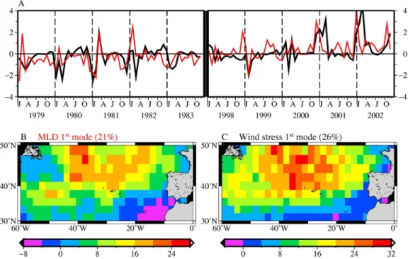
both parameters represents approximately the same amount of their total variance (21% and 26%, respectively, for the MLD and wind stress). Their spatial distributions both show high variability in the NADR region (Figures 9b and 9c). The MLD and wind stress time functions of the EOFs are driven by the high variability in the northeastern region (Figure 9a). They are accordingly correlated (r = 0.5). They show similar positive anomalies in the 2000s compared to the 1980s. The positive peaks from 2000 to 2002 both appear on the wind stress and MLD anomalies, suggesting that deeper MLD during the SeaWiFS era were related to stronger winds in the NADR region. This is actually what appears when comparing Figure 10 (Hovmoller plot of the wind stress) and Figures 6c and 6d. Winds were stronger in the 2000s than they were in the 1980s.
4.
Summary and Discussion
[31] In the NWCS region (roughly 38°N–50°N and 60°
W–40°W), the MLD characteristics only slightly differed between the CZCS and SeaWiFS eras. The amplitude of the fall and spring blooms was high during both periods, with little differences.
[32] In the eastern Atlantic (30°N–50°N and 40°W–0°W),
two blooms of similar amplitude occurred in fall and spring at the beginning of the 1980s (CZCS era, 1979–1983). At the beginning of the 2000s (SeaWiFS era, 1998–2002), the spring bloom was stronger and extended further south than Figure 7. Month of the occurrence of Chl maximum
reached between September and January and referred to as the fall bloom for (a) the CZCS era (1979–1983) and (b) the SeaWiFS era (1998–2002), as indicated. Black pixels are where no distinct fall bloom existed.
in the 1980s. This stronger spring Chl may be related to stronger wintertime winds, which induced deeper MLD, leading to enhanced nutrient uplift (bottom‐up process; e.g., Dutkiewicz et al. [2001]). The fall bloom was weaker in the 2000s and only appeared at the northern boundary of the study region. The MLD deepening at the end of summer has been delayed. It occurred 1 month later in 1998–2002 than in 1979–1983. This delay combined with a deeper winter MLD likely increased light limitation and consequently limited a full development of the fall bloom.
[33] The fall bloom is less documented in the literature
than the spring bloom. One possible reason is its small amplitude in the 2000s. The way in which time series are often analyzed might also be an explanation, as the usual representation uses plots starting in January, which emphasizes spring blooms, not fall or winter blooms. The weaker fall bloom in the 2000s than in the 1980s is con-sistent with a 1 month delay in the MLD deepening at the end of summer. This delay we observed in the NADR region has also been reported in the Mid‐Atlantic Bight by Schofield et al. [2008]. Although the difference in the timing Figure 9. (a) Time functions and spatial patterns of the (b) first nonseasonal mode of the MLD EOFs
(red curve in Figure 9a) and (c) wind stress EOFs (black curve in Figure 9a).
Figure 10. Latitude versus time plots of wind stress for the eastern Atlantic (average over 40°W–0°W) during the (a) CZCS and (b) SeaWiFS eras.
of the MLD deepening in fall has been put forward here as one possible explanation for the much lower fall bloom in the 2000s, other causes are possible. They include lateral advection [Williams and Follows, 1998; Dutkiewicz et al., 2001], mesoscale motions [McGillicuddy and Robinson, 1997], or wind bursts and storms, which all influence the timing of the ML shoaling [Lévy et al., 2005] and can impact the bloom dynamics. One of the most obvious forcing of the differences in the phytoplankton fall bloom would be the frequency of wind bursts in fall and winter, particularly north of 40°N [Lévy et al., 2005]. However, the investigation of the frequency of the wind bursts is impeded by the unavailability of high‐quality long‐term wind records with a sufficiently high temporal resolution.
[34] The absence of a fall bloom in the 2000s could also
be due to changes in zooplankton populations [Beaugrand et al., 2002]. Over the decades from the 1950s to the present, the cold water species (Calanus finmarchicus), which has a single peak of abundance in spring, has been replaced by a warm water species (Calanus helgolandicus) characterized by two peaks of abundance in spring and fall [Planque and Fromentin, 1996]. These changes of domi-nance in zooplankton communities reported in parallel to the Northern Hemisphere warming might explain an increase in grazing pressure in fall that would have prevented the bloom development in this season in the northeastern Atlantic.
[35] The spring bloom differences in the eastern Atlantic
are more likely related to differences in the physical envi-ronment (bottom‐up processes). As explained in the intro-duction, an inverse relationship between Chl and SST is usually expected, whereas in the North Atlantic higher SST and Chl were reported in the 2000s as compared to the 1980s and related to a regime shift of the Atlantic Multi-decadal Oscillation (AMO) from a cold to a warm phase in the mid‐1980s [Martinez et al., 2009]. The usual scenario would have predicted a shallower MLD and weaker Chl in the subtropical region and enhanced Chl in the subpolar region. Our results show that SST was higher in the 2000s than it was in the 1980s, in parallel to stronger winds and deeper winter MLDmax. As the present study focuses on two
5 year time periods separated by about 15 years, these dif-ferences might simply reflect interannual variability. How-ever, the correlative deeper MLD and stronger winds that we observed here were also reported over a longer and unin-terrupted time series (1960–2004) in this region [Yu, 2007; Carton et al., 2008]. These results show that our observa-tions might as well be related to a long‐term change.
[36] Finally, the impact of the differences in Chl, SST,
and MLD on the modeled annual primary production over the entire study region and for clear‐sky conditions is lim-ited, with a∼5% increase from an average of 2.41 GtC over 1979–1983 to 2.54 GtC over 1998–2002. Under overcast conditions (as a sensitivity test), the modeled annual pri-mary production is also slightly higher (by ∼7%) in the 2000s than in the 1980s. The higher SST related with a deeper MLD in the 2000s than in the 1980s in the north-eastern Atlantic illustrates that SST can be an ambiguous indicator of stratification. It also highlights the complexity of the links between SST changes, upper layer stratification, and biological responses. This study focused on the North Atlantic, where parallel higher Chl‐SST has been shown
from the CZCS to the SeaWiFS era [Martinez et al., 2009]. Parallel lower Chl‐SST has also been reported in other areas. All together, the regions with a parallel time evolu-tion of Chl and SST represent about 40% of the perma-nently stratified waters [Martinez et al., 2009]. Further studies are therefore needed in these areas (the Indian Ocean for instance).
[37] Acknowledgments. We thank Annick Bricaud, Joséphine Ras, and three anonymous reviewers for their comments on this manuscript. This work has been performed in the frame of the GLOBPHY project, which was funded by the Agence Nationale de la Recherche (ANR, Paris). EM was also supported by the Changing Earth Science Network initiative funded by the Support To Science Element (STSE) program of the Euro-pean Space Agency (ESA). This work was supported by the Centre National d’Etudes Spatiales (CNES).
References
Antoine, D., and A. Morel (1996), Oceanic primary production: 1. Adaptation of a spectral light‐photosynthesis model in view of appli-cation to satellite chlorophyll observations, Global Biogeochem. Cycles, 10, 43–55, doi:10.1029/95GB02831.
Antoine, D., A. Morel, H. R. Gordon, V. F. Banzon, and R. H. Evans (2005), Bridging ocean color observations of the 1980s and 2000s in search of long‐term trends, J. Geophys. Res., 110, C06009, doi:10.1029/ 2004JC002620.
Banse, K. (1992), Grazing, temporal changes of phytoplankton concentra-tions, and the microbial loop in the open sea, in Primary Productivity and Biogeochemical Cycles in the Sea, edited by P. G. Falkowski and A. D. Woodhead, pp. 409–440, Plenum, New York.
Beaugrand, G., P. C. Reid, F. Ibanez, J. A. Lindley, and M. Edwards (2002), Reorganization of North Atlantic marine copepod biodiversity and climate, Science, 296, 1692–1694, doi:10.1126/science.1071329. Behrenfeld, M. J. (2010), Abandoning Sverdrup’s critical depth
hypothe-sis on phytoplankton blooms, Ecology, 91(4), 977–989, doi:10.1890/09-1207.1.
Behrenfeld, M. J., R. T. O’Malley, D. A. Siegel, C. R. McClain, J. L. Sarmiento, G. C. Feldman, A. J. Milligan, P. G. Falkowski, R. M. Letelier, and E. S. Boss (2006), Climate‐driven trends in contemporary ocean productivity, Nature, 444(7120), 752–755, doi:10.1038/ nature05317.
Carton, J. A., S. A. Grodsky, and H. Liu (2008), Variability of the oceanic mixed layer, 1960–2004, J. Clim., 21, 1029–1047, doi:10.1175/ 2007JCLI1798.1.
Colebrook, J. M. (1979), Continuous plankton records: Seasonal cycles of phytoplankton and copepods in the Atlantic Ocean and North Sea, Mar. Biol. Berlin, 51, 23–32, doi:10.1007/BF00389027.
Colebrook, J. M. (1982), Continuous plankton records: Seasonal variations in the distribution and abundance of plankton in the North Atlantic Ocean and the North Sea, J. Plankton Res., 4, 435–462, doi:10.1093/plankt/ 4.3.435.
Dandonneau, Y., P.‐Y. Deschamps, J.‐M. Nicolas, H. Loisel, J. Blanchot, Y. Montel, F. Thieuleux, and G. Bécu (2004), Seasonal and interannual variability of ocean color and composition of phytoplankton communities in the North Atlantic, equatorial Pacific and South Pacific, Deep Sea Res. Part II, 51, 303–318.
de Boyer Montégut, C., G. Madec, A. S. Fischer, A. Lazar, and D. Iudicone (2004), Mixed layer depth over the global ocean: An examination of pro-file data and a propro-file‐based climatology, J. Geophys. Res., 109, C12003, doi:10.1029/2004JC002378.
Doney, S. C. (2006), Oceanography: Plankton in a warmer world, Nature, 444, 695–696, doi:10.1038/444695a.
Ducklow, H. W., and R. P. Harris (1993), Introduction to the JGOFS North Atlantic bloom experiment, Deep Sea Res. Part II, 40, 1–8, doi:10.1016/ 0967-0645(93)90003-6.
Dutkiewicz, S., M. Follows, J. Marshall, and W. W. Gregg (2001), Interan-nual variability of phytoplankton abundances in the North Atlantic, Deep Sea Res. Part II, 48, 2323–2344, doi:10.1016/S0967-0645(00)00178-8. Follows, M., and S. Dutkiewicz (2001), Meteorological modulation of the
North Atlantic spring bloom, Deep Sea Res. Part II, 49, 321–344, doi:10.1016/S0967-0645(01)00105-9.
Gregg, W., and K. Carder (1990), A simple spectral solar irradiance model for cloudless maritime atmospheres, Limnol. Oceanogr., 35, 1657–1675, doi:10.4319/lo.1990.35.8.1657.
Hovis, W. A., et al. (1980), Nimbus‐7 coastal zone color scanner: System description and initial imagery, Science, 210(4465), 60–63, doi:10.1126/ science.210.4465.60.
Kennelly, M. A., J. A. Yoder, B. M. Uz, and S. Doney (2000), Satellite studies of winter–spring phytoplankton chlorophyll transitions in the north Atlantic, Eos Trans. AGU, 80(49), Ocean Sci. Meet. Suppl., Abstract OS64.
Lévy, M., Y. Lehahn, J.‐M. André, L. Mémery, H. Loisel, and E. Heifetz (2005), Production regimes in the northeast Atlantic: A study based on Sea‐viewing Wide Field‐of‐view Sensor (SeaWiFS) chlorophyll and ocean general circulation model mixed layer depth, J. Geophys. Res., 110, C07S10, doi:10.1029/2004JC002771.
Longhurst, A. (1995), Seasonal cycles of pelagic production and consump-tion, Prog. Oceanogr., 36, 77–167, doi:10.1016/0079-6611(95)00015-1. Martinez, E., D. Antoine, F. D’Ortenzio, and B. Gentili (2009), Climate‐ driven basin‐scale decadal oscillations of oceanic phytoplankton, Science, 326, 1253–1256, doi:10.1126/science.1177012.
McClain, C. R., G. Feldman, and S. Hooker (2004), An overview of the SeaWiFS project and strategies for producing a climate research quality global ocean bio‐optical time series, Deep Sea Res. Part II, 51, 5–42, doi:10.1016/j.dsr2.2003.11.001.
McGillicuddy, D. J., and A. R. Robinson (1997), Eddy induced nutrient supply and new production in the sargasso sea, Deep Sea Res. Part I, 44, 1427–1450, doi:10.1016/S0967-0637(97)00024-1.
Morel, A. (1991), Light and marine photosynthesis: A spectral model with geochemical and climatological implications, Prog. Oceanogr., 26, 263–306, doi:10.1016/0079-6611(91)90004-6.
Planque, B., and J. P. Fromentin (1996), Calanus and environment in the eastern North Atlantic. Part I. Spatial and temporal patterns of C. fin-marchicus and C. Helgolandicus, Mar. Ecol. Prog. Ser., 134, 101–109, doi:10.3354/meps134101.
Polovina, J. J., G. T. Mitchum, and G. T. Evans (1995), Decadal and basin‐ scale variation in mixed layer depth and the impact on biological produc-tion in the central and North Pacific, 1960–88, Deep Sea Res. Part I, 42, 1701–1716, doi:10.1016/0967-0637(95)00075-H.
Polovina, J. J., E. A. Howell, and M. Abecassis (2008), Ocean’s least pro-ductive waters are expanding, Geophys. Res. Lett., 35, L03618, doi:10.1029/2007GL031745.
Richardson, A. J., and D. S. Schoeman (2004), Climate impact on plankton ecosystems in the northeast Atlantic, Science, 305, 1609–1612, doi:10.1126/science.1100958.
Rossow, W. B., and R. A. Schiffer (1999), Advances in understanding clouds from ISCCP, Bull. Am. Meteorol. Soc., 80, 2261–2288. Sarmiento, J. L., et al. (2004), Response of ocean ecosystems to climate
warming, Global Biogeochem. Cycles, 18, GB3003, doi:10.1029/ 2003GB002134.
Schofield, O., et al. (2008), The decadal view of the Mid‐Atlantic Bight from the COOLroom: Is our coastal system changing?, Oceanography, 21(4), 108–117.
Siegel, D. A., S. C. Doney, and J. A. Yoder (2002), The North Atlantic spring phytoplankton bloom and Sverdrup’s critical depth hypothesis, Science, 296, 730–733, doi:10.1126/science.1069174.
Sverdrup, H. U. (1953), On conditions for the vernal blooming of phyto-plankton, ICES J. Mar. Sci., 18, 287–295.
Ueyama, R., and B. C. Monger (2005), Wind‐induced modulation of sea-sonal phytoplankton blooms in the North Atlantic derived from satellite observation, Limnol. Oceanogr., 50(6), 1820–1829, doi:10.4319/ lo.2005.50.6.1820.
Williams, R. G., and M. J. Follows (1998), The Ekman transfer of nutrients and maintenance of new production over the North Atlantic, Deep Sea Res. Part I, 45, 461–489, doi:10.1016/S0967-0637(97)00094-0. Woodruff, S. D., et al. (2010), ICOADS release 2.5: Extensions and
enhancements to the surface marine meteorological archive, Int. J. Cli-matol., 31(7), 951–967, doi:10.1002/joc.2103.
Yoder, J. A., C. R. McClain, G. C. Feldman, and W. E. Esaias (1993), Annual cycles of phytoplankton chlorophyll concentrations in the global ocean–a satellite view, Global Biogeochem. Cycles, 7, 181–193, doi:10.1029/93GB02358.
Yu, L. (2007), Global variations in oceanic evaporation (1958–2005): The role of the changing wind speed, J. Clim., 20, 5376–5390, doi:10.1175/ 2007JCLI1714.1.
D . A n t o i n e , F . D’Ortenzio, and E. Martinez, Laboratoire d’Océanographie de Villefranche, UMR 7093, CNRS, UPMC, Université de Paris, Villefranche‐sur‐Mer F‐06230, France. (martinez@obs‐vlfr.fr)
C. de Boyer Montégut, Laboratoire d’Océanographie Spatiale, IFREMER, Brest Center, Pointe du Diable, B.P. 70, Plouzané F‐29280, France.