Advances in fully-kinetic PIC simulations of near-vacuum Hall thruster and other plasma systems

Advances in Fully-Kinetic PIC Simulations of a

Near-Vacuum Hall Thruster and Other Plasma Systems

by

Justin

M. Fox

B.S., California Institute of Technology (2003)

S.M., Massachusetts Institute of Technology (2005)

Submitted to the Department of Aeronautics and Astronautics

in partial fulfillment of the requirements for the degree of

Doctor of Philosophy in Aeronautics and Astronautics

at the

MASSACHUSETTS INSTITUTE OF TECHNOLOGY

June 2007

© Massachusetts Institute of Technology 2007, All rights reserved.

Author ... ... .. .. ... ...

Department of Aeronautics and Astronautics

June 11, 2007

Certified by ... ... . . . . . . . . . .

Manuel Martinez-Sanchez

Professor of Aeronautics and Astronautics

/esis

Supervisor

Certified by ...

Oleg Batishchev

Principal Research Scientist

Supervisor

NOV 0 6

₂

Jaime Peraire

Professor of Aeronautics and Astronautics

Chair, Committee on Graduate Students

Advances in Fully-Kinetic PIC Simulations of a

Near-Vacuum Hall Thruster and Other Plasma Systems

by

Justin M. Fox

Submitted to the Department of Aeronautics and Astronautics on June 11, 2007, in partial fulfillment of the

requirements for the degree of

Doctor of Philosophy in Aeronautics and Astronautics

Abstract

In recent years, many groups have numerically modeled the near-anode region of a Hall thruster in attempts to better understand the associated physics of thruster operation. Originally, simulations assumed a continuum approximation for electrons and used magnetohydrodynamic fluid equations to model the significant processes. While these codes were computationally efficient, their applicability to non-equilibrated regions of the thruster, such as wall sheaths, was limited, and their accuracy was predicated upon the notion that the energy distributions of the various species remained Maxwellian at all times. The next generation of simulations used the fully-kinetic particle-in-cell (PIC) model. Although much more computationally expensive than the fluid codes, the full-PIC codes allowed for non-equilibrated thruster regions and did not rely on Maxwellian distributions. However, these simulations suffered for two main reasons. First, due to the high computational cost, fine meshing near boundaries which would have been required to properly resolve wall sheaths was often not attempted. Second, PIC is inherently a statistically noisy method and often the extreme tails of energy distributions would not be adequately sampled due to high energy particle dissipation.

The current work initiates a third generation of Hall thruster simulation. A PIC-Vlasov hybrid model was implemented utilizing adaptive meshing techniques to enable automatically scalable resolution of fine structures during the simulation. The code retained the accuracy and versatility of a PIC simulation while intermittently recalculating and smoothing particle distribution functions within individual cells to ensure full velocity space coverage. In addition, this simulation extended the state of the art in Hall thruster anomalous diffusion modeling by adopting a "quench rule" which is able to predict the spatial and temporal structure of the cross-field transport without the aid of prior empirical data. Truly predictive computations are thus enabled. After being thoroughly tested and benchmarked, the simulation was then applied to the near vacuum Hall thruster recently constructed at MIT. Recommendations to improve that thruster's performance were made based on the simulation's results, and those optimizations are being experimentally implemented by other researchers.

This work was conducted with the aid of Delta Search Labs' supercomputing facility and technical expertise. The simulation was fully-parallelized using MPI and tested on a 128 processor SGI Origin machine. We gratefully acknowledge that funding for portions of this work has been provided by the United States Air Force and the National Science Foundation.

Thesis Supervisor: Manuel Martinez-Sanchez Title: Professor of Aeronautics and Astronautics Thesis Supervisor: Oleg Batishchev

Acknowledgments

What a long road it has been...one that I could never have walked alone. I want to first thank my advisor Professor Martinez-Sanchez for his invaluable guidance and for the opportunity to conduct this research. For Dr. Oleg Batishchev, my co-advisor, and his wife Dr. Alla Batishcheva, my "boss," words cannot even express the depth of my gratitude. Two more hard-working, generous, and kind-hearted individuals I could never hope to meet again, and I can't thank them enough for everything they have done for me and my wife. I hope this thesis brings them some small amount of happiness and pride, for without their steadfast support, none of this would have been possible!

I must further thank my colleagues in the Space Propulsion Lab for all of their

help and friendship along the way. I wish them all luck wherever their next adventures may lead. A very special thanks also to Kamal Jaffrey and my other friends at Delta Search Labs for their generosity, laughter, and faithful support throughout my research here at MIT. I also must acknowledge the National Science Foundation for funding the majority of this research.

Of course, last but certainly not least, I'd like to thank my family. I am so

fortunate to have those around me who have been willing to set aside their own happiness and own agendas to give me the chance to make this long journey. My mother and father have sacrificed so much for their two sons over the years, and I am filled with nothing but the profoundest pride, respect, and love for them. No child could have been more loved. To my newly-wedded wife who lovingly followed me to this strange northern land and braved its frigid wonders with an open and adoring heart, thank you! I can't wait to begin our next adventure together, hand in hand, forever and always.

And if there's anyone I haven't mentioned, it's only because there's not enough paper in the world to thank everyone who has helped me along the way! Thank you all so very much!

Contents

1

Introduction

31

1.1 What is a Plasma? 31

1.2 General Equations of Plasmas 33

1.3 Hall-Effect Thrusters 35

1.4 The Near Vacuum Hall Thruster 36

1.5 Previous Hall Thruster Modeling 38

1.6 Goals of Present Thesis 39

1.7 Summary of Methodology 41

1.7.1 Basic Simulation Flow Chart 41

1.7.2 New Features of the Grid 44

1.7.3 Particle Weighting and Redistribution 45

1.7.4 New Collisional Model 46

1.7.5 Anomalous Diffusion Modeling 48

1.7.6 Parallelization 49 1.8 Summary of Tools 50 1.8.1 Hardware 50 1.8.2 Software 51 1.9 Summary of Results 51 1.9.1 Code Validation 52

1.9.2 Anomalous Diffusion Model 52

1.9.3 Near Vacuum Hall Thruster 53

2

Numerical Method

55

2.1 General Mesh Structure and Creation 55

2.1.1 Example Meshes and Qualitative Correctness

2.2 Recursive Refinement and Coarsening Procedure 60

2.2.1 Details of the RRC Technique 61

2.2.2 Conservation of Splined Quantities Across Cell Faces 63

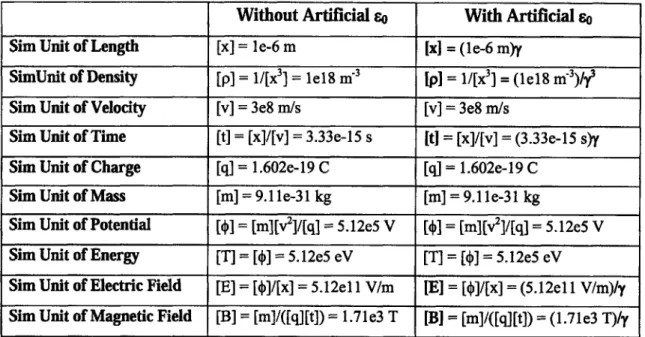
2.3 Simulation units 67

2.3.1 Length Scale 68

2.3.2 Time Scale 69

2.3.3 Other Derived Units 69

2.4 Acceleration Techniques 70

2.4.1 Reducing the Simulated Particle Number - Statistical

Weighting 70

2.4.2 Artificial Permittivity 71

2.4.3 Artificial Mass Ratio 73

2.5 Semi-analytic Particle Trajectory Integrator 74

2.5.1 Semi-Analytical Relativistic Orbit Integrator for a 2D2V

System 75

2.5.1.1 Half Step in Electric Field 77 2.5.1.2 Full Step in Magnetic Field 78 2.5.2 Analytical Orbit Integrator in the Classical 3D3V Case 79 2.5.3 Semi-Analytic Orbit Integrator for the Relativistic 3D3V

Case 80

2.5.3.1 Half Step Acceleration in Electric Field 80 2.5.3.2 Full Step Rotation of Velocity Vector in Magnetic

Field 80

2.5.4 2D3V Methodology 81

2.6 Particle-in-Cell Weighting Scheme 83

2.6.1 Weighting Scheme in 2D 83

2.6.2 Weighting Scheme for RZ Geometries 86 2.7 Self-Consistent Calculation of Electric field 88 2.7.1 Approximations to Gauss's Law 89

2.7.1.1 Approximating Gauss's Law using Simple Linear

2.7.1.2 Approximating Gauss's Law using Splines 92 2.7.1.3 Using Splines for an Axisymmetric Geometry 95 2.7.2 Solving the Resulting Matrix Equations 96 2.7.2.1 Successive Over-Relaxation Overview 96 2.7.2.2 Direct Solution Technique Using MUMPS 97 2.7.3 Approximating the Electric Field from a Given Electric

Potential 98

2.8 Models for Collision Events 101

2.8.1 Intra-Species Elastic Collisions 102

2.8.2 Neutral-Electron Inelastic Collisions 104

2.8.2.1 Creation of Cold Secondary Electrons Through

Collisions 107

2.8.2.2 Semi-Analytical Equations For Electron Impact

Collisions 107

2.8.2.3 Calculating the Individual Rates 110 2.8.3 Compiling Cross-Sections 112

2.8.3.1 Total Cross-Section Data 113 2.8.3.2 Elastic Cross-Section Data 115

2.8.3.3 Ionization Cross-Section Data 115

2.8.3.4 Excitation Cross-Section Data 117

2.8.3.5 Inclusion of Cross-Sections Into Simulation 118

2.9 Velocity Redistribution Step 122

2.10 Addition of Particles 126

2.10.1 Initial Conditions 126

2.10.2 Injection of Neutrals 129

2.10.3 Injection of Cathode Electrons 129

2.10.4 Injected Particles' Initial Distribution 130

2.11 Boundary Conditions 131

2.11.1 SPACE - Free Space Condition 132

2.11.2 METAL - Floating Metallic conductor 132 2.11.3 DIELE - Dielectric Insulator 133

2.11.4 CATHO - Implicit Cathode

2.11.5 ANODE - Fixed-Potential Metal Anode 2.12 Data Collection

2.12.1 Output Files Defined

2.13 Parallelization

2.13.1 Comparing MPI Functions Using CVPerf 2.13.2 Initialization

2.13.3 Particle Injection

2.13.4 Collisions, Vlasov Step, and Scattering

2.13.5 Field Solution 2.13.6 Load Rebalancing 2.13.7 Particle Movement

3

Code Validations

3.1 Constant Field Particle Motion Integrator Tests

3.1.1 Two-Dimensional Integrator - Zero Fields

3.1.2 Two-Dimensional Integrator - Zero Fields with Adaptation

3.1.3 Two-Dimensional Integrator - Constant B-Field 3.1.4 Two-Dimensional Integrator - Constant ExB Field

3.1.5 Axisymmetric Integrator - Zero Fields

3.1.6 Axisymmetric Integrator - Constant B-Field

3.1.7 Axisymmetric Integrator - Checking Mass

3.2 Electric Potential and Field Solution Tests

3.2.1 Examining Solution Convergence on Refined Meshes

3.2.2 Patching the Spline Method for Adapted Grids

3.2.3 Testing the Patched Spline Method on Adapted Grids 3.2.4 Testing the Calculation of Electric Field from the Given

Potential

3.2.5 Testing the Axisymmetric Patched Spline Method 3.2.6 Comparing the Iterative and Direct Solution Techniques

135 135 135 136 138 139 140 142 143 143 145 147

149

3.3 Self-Consistent Field Calculation Tests 175 3.3.1 Self-Consistent Single Particle Motion Test 176 3.3.2 2D Langmuir Oscillation Tests 178 3.3.3 RZ Langmuir Oscillation Tests 183

3.4 Neutral-Neutral Elastic Collision Testing 184

3.4.1 Conservation Tests 185

3.4.2 Neutrals in a 2D Box Test 186

3.4.3 Neutrals in an RZ Box Test 189

3.4.4 Flow Past A Backward-Facing Step 191

3.4.5 Flow Through A Choked Nozzle 193

3.5 Wall Sheath Test 195

3.5.1 Test Set-up 196

3.5.2 Initial Results 197

3.5.3 Addition of Quasi-Coulomb Collisions and Finalized

Results 200

3.6 Velocity Redistribution Step Conservations 204

3.7 Parallelization Benchmarking 206

3.7.1 Timing the RZ Particle Movement Module 207

3.7.2 Timing the MUMPS Solver 209

3.7.3 Timing the Collision Module 212 3.7.4 Timing the Velocity Redistribution Module 214

3.7.5 Load Balancing Test 214

4

System-level Benchmarking Using the P5 Thruster

217

4.1 Details of the P5 Thruster 218

4.1.1 Geometry and Mesh 219

4.1.2 Magnetic Field 222

4.1.3 Special P5 Simulation Conditions 223

4.1.3.1 Dielectric Boundary and Potential Calculation 223

4.1.3.2 Secondary Electron Emission 227

4.1.3.4 P5 Cathode and Free Space Boundary Condition 4.2 Comparison of Current Work with PIC-MCC Simulation and

Experiment

4.2.1 Electric Potential 4.2.2 Particle Densities 4.2.3 Electron Temperature

5

Near Vacuum Hall Thruster Simulations

5.1 Previous Experimental Work

5.2 Details of the NVHT

5.2.1 Geometry and Mesh

5.2.2 Magnetic Field

5.2.3 Update to the Theoretical Model for the NVHT

5.2.4 Mean Free Path Analysis

5.2.5 Special NVHT Simulation Conditions

5.2.5.1 NVHT Implicit Cathode Condition

5.2.5.2 Background Neutral Density Approximation

5.3 Initial Simulation Results

5.3.1 Electric Potential 5.3.2 Ionization Zone 5.3.3 Ion Energies 5.3.4 Particle Densities 5.3.5 Electron Temperature 5.4 Re-Design Recommendations

5.5 Simulation Results After Re-Design

5.5.1 Electric Potential

5.5.2 Ionization Zone

5.5.3 Ion Energies

5.5.4 Particle Densities

5.5.5 Electron Temperature

5.5.6 Results at Lower Anode Potential

230 231 231 232 235

237

6

Novel Anomalous Diffusion Model for Hall Thruster

Simulations

271

6.1 Explanation of Anomalous Diffusion 272

6.2 Bohm's Model of Diffusion 272

6.3 Previous Simulation Techniques 274

6.4 Goal of the Present Technique 278

6.5 Correlation of ExB Shear and Transport in Hall Thrusters 280

6.6 Quench Model 280

6.6.1 History and Background 281

6.6.2 The Quench Model in a Hall Thruster Geometry 282 6.6.3 Selecting the Oscillatory Mode 283

6.6.4 Maximum Linear Growth Rate of Transit-Time

Oscillations 285

6.6.5 Averaging the Electric Field 286

6.6.6 Putting It All Together - Implementation in the Code 288 6.7 P5 Results Demonstrating Quench Model Performance 289 6.7.1 Transient Diffusion Barriers 289 6.7.2 Comparing Temperature and Potential Profiles 292 6.7.3 Comparing Current and Thrust Predictions 297 6.8 Evaluation of the Quench Model's Viability 300

7

Conclusions and Future Work

302

7.1 Unique Numerical Advances 302

7.2 Results from Application of the Simulation 303

7.3 Recommended Future Tasks 304

A

Usage of Tecplot Mesh Generator Add-on

307

B

Tables of Compiled Experimental Cross-Sections

316

C

Simulated Distribution Functions for the P5 Thruster

319

List of Figures

1-1 A schematic representation of a Hall thruster. 36

1-2 A high-level flowchart of the simulation. 42

1-3 A graphical representation of the splitting procedure that occurs during

neutral-electron inelastic collisions. This differs from the typical Monte Carlo

model in that instead of all of a fraction of the particles colliding, our model 47 collides a fraction of all of the particles, thus eliminating one source of

statistical noise.

2-1 _{Example unstructured, quadrilateral meshes for (a) pseudospark device,}

(b) Hall thruster with central cathode, and (c) other difficult or awkward 56

geometries.

2-2 Three different particle trajectories are here overlayed on a Tecplot Mesh Generator generated mesh. The adaptation region lies between 5 and 9 x units. There is no electric field present in this trial and the B-field is directed

58

out of the page. The particle trajectories should therefore be perfect circles as they are seen to be. Each of the three particles has a different initial velocity accounting for the varying path radii.

2-3 This test added a small electric field in the y-direction to the test above. Again the particles have differing initial velocities accounting for the difference in radius. The particles are easily able to move from cell to cell and

59

from zone to zone in this multi-zone quadrilateral mesh, illustrating that our functions are capable of maintaining the mesh structure as well as properly calculating the neighboring element array.

meshes can be integrated with our computational model's cluster adaptation.

2-5 One final demonstration. The particle is easily able to traverse the

multiple zones of this mesh and pass through the multiple regions of 60

adaptation.

2-6 An example of the static local-refinement employed in some NVHT tests. For the results presented in this thesis, we did not allow the mesh to

adapt automatically as in full RRC, but the simulation was designed to allow 61

such automatic adaptation and all solvers and algorithms were implemented with this technique in mind.

2-7 An example RRC mesh demonstrating both (a) a regular six-point stencil for a cell face and (b) an irregular five-point stencil for a cell face.

Since RRC guarantees that refinement level only changes by +/- 1 from 63

neighbor to neighbor, these two stencil cases are the only two that need to be considered with the exception of boundary elements and faces.

2-8 The definition of the points in the two spline functions (a) S and (b) F. 64

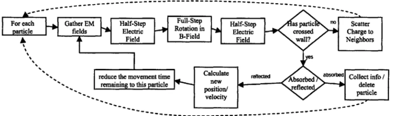
2-9 A flowchart depicting the particle movement process in the serial

75

implementation.

2-10 Particle motion physically in the 0-direction is folded back into the

RZ-plane and becomes motion in the positive R-direction under the 2D3V 82

assumption.

2-11 Under the inverse-distance weighting scheme, the weighting factors could change non-smoothly even during an infinitesimal particle motion.

84 These discontinuities in weighting sometimes led to a significant self-force

being calculated on an individual particle.

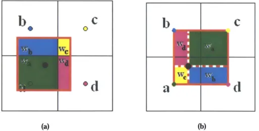
2-12 Illustration of PIC-weighting method. (a) Conceptually, we calculate the overlapping volume of a particle with the neighboring cells. (b) For the

general refined and non-orthogonal case, a different computational 85

implementation is actually used to compute the weights which does reduce in the simple case to an overlapping volume scheme.

2-14 The density after scattering for a uniform distribution of neutrals was

calculated using (a) the naive generalization of the two-dimensional scheme 87

and (b) a method which accounts for the RZ geometry.

2-15 The gradient in potential between cell s and cell n must be integrated 90

over facet 1-2.

2-16 A five-point stencil for spline approximation of the electric field. 99 2-17 The five-point stencil is turned into four three-point stencils in order to

100 avoid ill-conditioned approximation matrices.

2-18 A flowchart showing the steps in the intra-species elastic collision

102 model.

2-19 The number of computational particles versus time for a simulation

104 with neutral-neutral elastic collisions.

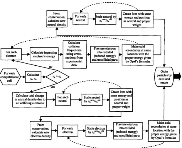
2-20 A flowchart depicting the basic steps of the complicated

neutral-105 electron inelastic collision method.

2-21 The percent error incurred if the linear approximation is used to

calculate the amount of each type of collision. In regions of high collisionality, 112 such as the ionization zone, this error can reach very significant levels.

2-22 Total cross-section data for (a) Xenon and (b) Krypton. 114

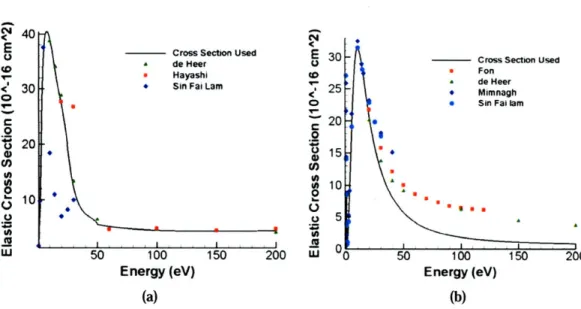
2-23 Elastic cross-section data for (a) Xenon and (b) Krypton. 116

2-24 Ionization cross-section data for (a) Xenon and (b) Krypton broken

117 down by ionization level. All data was taken from Rejoub's 2001 study.

2-25 The polynomial fit cross-sections for (a) Xenon and (b) Krypton. The

jaggedness and possible inaccuracy of these polynomial fits prompted the 119

creation of the second, more intensive interpolation algorithm described below.

2-26 _{The final compiled cross-section data for (a)-(c) Krypton and (d)-(f)}

Xenon. The cross-sections for (a)(d) Excitation, (b)(e) Ionization, and (c)(f) 121 the total for classical collisions are shown.

2-27 The experimental elastic cross-section data compared to the actual

122 cross-section employed by the simulation for (a) Xenon and (b) Krypton.

module.

2-29 Velocity space redistribution is accomplished by particles in a given cell first being placed on a velocity grid. Velocity space cells having more

125 than two particles then have their particles combined while energy,

momentum, and density are retained.

2-30 The diagram illustrates the discretization of the initial Maxwellian distribution during particle creation. The red dots on the velocity axis indicate the 6 particles that are created. The range of velocities is specified by v_half_ v

127 and the number of grid cells is controlled by n&halfv. The initial statistical

weight assigned to a particle, being the value of the Maxwellian at that point, is shown by the dotted line as well.

2-31 A plot depicting the strong co-variance of the anode and cathode

currents along with the beam and ionization currents. This plot was generously 135

created and provided by Szabo.

2-32 The percentage of the total particles being transferred between processors at each time step is displayed for trials with (a) 8 processors and (b)

16 processors. Note that the horizontal axes of these figures are different. The

periodic sharp peaks are due to the re-weighting of neutral particles which 146

occurs relatively infrequently, but significantly alters the particle number on each processor requiring greater than usual particle transfer to rebalance the

load.

3-1 (a) Three different charged particles released at the same time in zero

electric and magnetic field all travel at the same rate and in straight lines. All

150

three reached the mesh edge at precisely the same moment in the simulation. (b) The relative error in impact time decreases with decreasing time step.

3-2 (a) Three particles were released in zero field on an adapted mesh. All

three reached the mesh boundary at the same time. (b) The relative error in

151

the time elapsed before the particles impacted the boundary decreases with decreasing time step.

3-3 (a) The trajectories of the three described particles in a field of B, = .2

Tesla. (b) The relative error in the calculated Larmor radius is reduced with 153

reducing time steps.

3-4 (a) 'The trajectories of the three described particles undergoing ExB

drift. (b) The time-averaged x-velocity (shown for the electron) tends to the 154 theoretical drift velocity on average.

3-5 (a) The trajectories of three particles using an axisymmetric solver

with no electromagnetic fields. (b) The relative error in the time until the 155

particles impacted the boundary is reduced with reduced time step.

3-6 The particles were given only x-directed velocity. The actual trajectory

then is just in the x-direction to the right toward the simulation boundary. 156

However, in the code, the particle is projected at each timestep back into the RZ plane and so only seems to move in the R-direction.

3-7 (a) The trajectories of three particles given only 8-directed velocities appear to be only in the R-direction after they have been projected onto the RZ plane. (b) Even though the particles were not all traveling in the same

157

direction and they traveled over different adaptation boundaries, they still arrived at the mesh boundary at the same moment. The error in this impact time was reduced with decreased time step.

3-8 (a) The negative particle (left) executes right-handed motion while the positive particle (right) executes left-handed motion about the magnetic field

158

which is directed into the drawing. (b) As the time step is decreased, the error in Larmor radius is decreased.

3-9 The trajectories of a negative particle (left) about a B, field and a

158

positive particle (right) about a BR field. The neutral particle is unaffected.

3-10 (a) The trajectories of two particles in a constant magnetic field. The green particle has twice the mass of the blue particle. (b) The computed

Larmor radius of both particles converges to the theoretical value with a small 160

3-11 The inner green trajectory was calculated with no artificial mass ratio. The outer blue trajectory was calculated with an artificial ratio of 1/25. The

161 only reason for the difference between the two is the relativistic effect of the

artificially lighter particle moving faster.

3-12 The normalized errors for each of the three successively refined meshes. (a) The coarse mesh has half as many elements as (b) the medium

162 mesh and a quarter as many elements as (c) the fine mesh. All three color

scales are the same allowing for direct comparison.

3-13 Average errors are plotted versus the base 2 log of the number of

elements. The error exhibits a roughly linear trend denoting an acceptable 163

convergence rate.

3-14 The definition of 0 accounts for the fact that our linear estimate of the

164 potential gradient is not actually normal to the facet.

3-15 Electric field created by uniformly-charged hollow cylinder 165 3-16 A mesh which yields singular spline matrices. The mesh is meant to be

completely regular with diamond shaped elements, leading to the spline matrix 167

shown in Equation 3.11.

3-17 The base mesh used for the charged cylinder, patched spline testing. 168 3-18 The normalized error between the analytic potential and calculated

potential for three successively refined meshes. (a) The coarse mesh has one

half as many elements as (b) the medium mesh and one quarter as many 169

elements as (c) the refined mesh. Note that the color scale is the same on all three meshes to enable direct comparison.

3-19 The average normalized errors for these three meshes plotted versus the

170 number of elements in the mesh on a log-log scale. The convergence is clear.

3-20 The normalized error between the analytic and calculated radial electric

field for three successively refined grids. Note that all three plots have the 171

same color scale.

generally covergent trend.

3-22 (a) The normalized error between the analytic and calculated potentials for an axisymmetric trial using only linear interpolation. (b) The error from a trial which employed the spline approximation in elements where the matrix

173 was non-singular and linear interpolation in the remaining elements. The

vertical axis is the r-direction, the horizontal axis is the z-direction and the symmetry axis is assumed to be horizontal along r=0.

3-23 (a) The analytic potential cos(nr) compared to (b) the calculated

174 potential with the boundaries set to this analytic potential..

3-24 (a) The normalized error calculated by comparing the analytical

potential cos(nr) to the value calculated by the direct solution technique using 174

MUMPS. (b) The same for the iterative SOR solver. Note that both (a) and (b) have the same color scale.

3-25 (a) The analytic potential r2_{cos(0) compared to (b) the calculated}

175 potential with this analytic potential on the boundary

3-26 (a) The normalized error calculated by comparing the analytical

potential r2_{cos(O) to the value calculated by the direct solution technique using 175}

MUMPS. (b) The same for the iterative SOR solver. Note that both (a) and (b) have the same color scale.

3-27 (a) The error in x-motion is small and can be arbitrarily reduced by

reducing the simulation time step. (b) The error in x-motion can also be 177

arbitrarily reduced by reducing the mesh spacing.

3-28 Electric Potential over time for a single particle in axisymmetric

177 geometry.

3-29 Norm of the electric field over time for a single particle in an

178 axisymmetric geometry.

3-30 _{The Potential at peak times separated by 16,750 simulation time steps,}

180 or about V2 of a plasma period.

3-31 The potential of a trial with a maximum refinement of four levels.

Notice that it is of course much smoother than the potential calculated with 181

less error. The mesh in these images is not shown since its fineness would obscure the image.

3-32 The simulation energies oscillate at the theoretical frequency, and the

181 total energy increases only slowly over time.

3-33 As the grid spacing is reduced, the plasma period becomes more

182 accurate.

3-34 (a) Ex and (b) Ey for the non-orthogonal Langmuir oscillation tests. 182 3-35 The total, kinetic, and potential energies over two plasma periods in the

183 non-orthogonal two-dimensional Langmuir oscillation test.

3-36 The initial potential for the RZ singly-adapted Langmuir oscillation

183 test.

3-37 (a) The energy for a three-level refined RZ Langmuir oscillation test.

(b) As the refinement was increased, the error in the calculated plasma period 184 was reduced.

3-38 Conservation of quantities during the neutral-neutral collision test. 186 3-39 The grid for the neutrals in a 2D box test was a simple square. The

187 density was roughly uniform at .1 simulation units.

3-40 The x-distribution function overlayed with a Maxwellian distribution

188 (dotted) as a function of time.

3-41 The relative L1 error between the neutrals' distribution function and a

188

true Maxwellian over time.

3-42 The two-dimensional distribution function as it changes from uniform

189 to Maxwellian due to neutral-neutral elastic collisions.

3-43 The initial density for the RZ neutrals in a box test. Note that the

density is smoother than in Figure N-I since there are more particles per cell in 190

this case to resolve the third dimension properly.

3-44 The x-distribution function overlayed with a Maxwellian distribution

190 (dotted) as a function of time for the RZ case.

3-45 The relative L1 error between the neutrals' distribution function and a

191 true Maxwellian over time for the RZ case.

to Maxwellian due to neutral-neutral elastic collisions for the RZ case.

3-47 The geometry for the backward-facing step neutral-neutral elastic

192

collision test.

3-48 _{The time-averaged, normalized neutral flow velocity with backstep 193} vortex streamline included.

3-49 (a) The normalized velocity for the backward facing step case. Two streamlines are shown, one which is trapped in the vortical structure and the

193 other which escapes. The reattachment point was approximately located at

x=8.6 for this case.

3-50 (a) Chamber density is uniform while plume density rapidly decreases.

(b) Flow accelerates to sonic velocity in the throat and is then further 194 accelerated in the expanding plume.

3-51 The mesh used for testing the sheath formation. Note that the scale on

the axes is different; the mesh can actually be very long and narrow since it is 197

periodic in the horizontal direction.

3-52 The normalized sheath potential at several evenly-spaced intervals is

199

highly oscillatory in this test. The mass ratio here was 1000.

3-53 The normalized sheath velocities and the time-averaged potentials for

the above sheath tests. The 1000 mass ratio case is shown in (a) and (c) while 200 the 10,000 mass ratio case is shown in (b) and (d).

3-54 The normalized sheath potential at several evenly-spaced time intervals is much more stable in this test. This figure shows results of the mass ratio

1000 test and can be compared to Figure 3-50 above. 201

3-55 The normalized sheath velocities and the time-averaged potentials for

the above sheath tests. The 1000 mass ratio case is shown in (a) and (c) while

the 10,000 mass ratio case is shown in (b) and (d). The heavy lines indicate 203

the sheath thickness is between 3 and 4 Debye lengths while the potentials calculated fall very nearly at the theoretical values expected.

3-56 Results of the velocity redistribution conservation tests. The (a)

density, (b) velocities, and (c) temperatures are conserved to very fine 205

has been reduced.

3-57 The raw timing results for the axisymmetric particle motion module.

Simulations with (a) 158,374 (b) 1,904,085, and (c) 20,324,568 particles were 208

conducted.

3-58 The parallel speed up of the axisymmetric particle motion module for

208 three different numbers of particles.

3-59 The raw timing results for the MUMPS solver and entire field solution

module. Simulations with (a) 5,535, (b) 48,621, and (c) 457,827 elements 211 were conducted.

3-60 The parallel speed up of the complete field solution module for three

211 different numbers of elements.

3-61 _{The raw timing results for the collision module. Simulations with (a) 213} 102,253 (b) 1,503,263, and (c) 10,364,653 particles were conducted.

3-62 The parallel speed up of the collision module for three different

213 numbers of particles.

3-63 The raw timing results for the velocity-redistribution module.

Simulations with (a) 102,253 (b) 1,503,263, and (c) 10,364,653 particles were 215

conducted.

3-64 The parallel speed up of the velocity-redistribution module for three

different numbers of particles. 215

3-65 The maximum percentage of particles being carried at each time step

by any processor. (a) 8 processor and (b) 16 processor tests were conducted.

The balance is roughly achieved, but is imperfect due to our requirement that 216

the particles within a given computational element not be split between processors.

4-1 A schematic representation showing the basic configuration of the P5

thruster being simulated. The geometry is axisymmetric assuming that the 220 cathode is implicitly modeled.

4-2 The computational meshes used in (a) the previous MIT PIC simulation

221 and (b) the present work.

4-3 The (a) radial and (b) axial magnetic field contours used for the P5

222 thruster.

4-4 The electric potential near the inner ring of the P5 thruster's channel. These results were obtained using the PIC-MCC simulation with (a) Blateau's original approximation and (b) the full calculation inside the dielectric. Much

thought and confusion had been invested in trying to understand why the 226

sheaths in the original simulation seemed to bend the wrong direction as the orange-yellow equipotential demonstrates in (a). This anomaly is no longer present if the full dielectric calculation is used.

4-5 _{The electric potential from (a) the former PIC-MCC model, (b) the}

232 present simulation, and (c) the experiments of Haas.

4-6 P5 Plasma densities calculated by the present simulation. The (a) ion

density and (b) electron density are slightly increased relative to previous 233

simulation results due to a better coverage of velocity space.

4-7 The doubly-charged ion density calculated by (a) the present simulation

234 and (b) Sullivan's PIC-MCC code.

4-8 The neutral density in the P5 thruster calculated using the present 235

numerical simulation.

4-9 The electron temperature for the P5 thruster from (a) the former

PIC-MCC simulation with constant Bohm approximation (b) the current simulation 237

with constant Bohm approximation and (c) the experiments of Haas.

5-1 _{The base grid for the NVHT. Both (a) the whole simulation and (b) the}

240 zoomed region around the thruster are shown.

5-2 The norm of the magnetic field in the channel of the NVHT. 242

5-3 The updated theoretical model for the NVHT current variation with

247 pressure agrees quite well with experiment.

5-4 The electric potential in the near-anode region of the NVHT. Note that

254 the scale in this figure is not linear.

5-5 Plots of the regions of (a) singly- and (b) doubly-charged ion

255

5-6 The raw RPA data reprinted from Sullivan and Bashir [7]. 256 5-7 The derived current vs. voltage data from Bashir and Sullivan's RPA

257

analysis [7].

5-8 The derivative of the current with respect to voltage as the voltage on

the simulated RPA was varied. This trial was conducted with a simulated tank 258

pressure of 1.1 * 1 0-4 torr and an anode voltage of 3.172kV.

5-9 The (a) electron, (b) singly-charged ion, and (c) doubly-charged ion

259

densities for the simulated near-vacuum Hall thruster.

5-10 The computed electron temperature for the near vacuum Hall thruster.

(a) The temperature outside the channel is generally less than 100eV while (b) 260

near the anode it can reach as much as 500eV.

5-11 The mesh of the redesigned NVHT featuring an anode which protrudes 262

farther into the channel.

5-12 The electric potential in the re-designed NVHT. 264

5-13 _{The (a) singly-charged and (b) doubly-charged ion production regions 265}

for the newly-designed NVHT with protruding anode.

5-14 For the re-designed NVHT, this plot shows the derivative of the current

266 with respect to voltage as the voltage on the simulated RPA was varied.

5-15 The (a) electron, (b) singly-charged ion, and (c) doubly-charged ion

268 densities for the re-designed near-vacuum Hall thruster.

5-16 The computed electron temperature for the re-designed near vacuum

Hall thruster. (a) The temperature outside the channel is generally less than 269

150eV while (b) near the anode it can reach as much as 500eV.

5-17 The simulated RPA analysis of the two NVHT designs at 2kV anode

270 potential.

5-18 The predicted (a) anode current and (b) thrust for the two thruster

270 designs at 2kV anode potential.

6-1 The dependence of the former MIT simulation's calculated electron

277 temperature on the spatial profile of the Bohm coefficient is very strong. (a)

An experimentally acquired plot (courtesy of Haas [37]) of the electron temperature with a peak temperature of roughly 30eV occurring near the exit of the channel. The former MIT simulation's calculation of the electron temperature is shown using (b) a spatially constant Bohm coefficient recommended by Sullivan and (c) an expertly-selected Bohm coefficient profile.

6-2 The three Hall parameter profiles used to compute the results shown in

278 Figure 6-3

6-3 The results computed by the former MIT simulation using the spatial

Hall parameter profiles depicted in Figure 6-2. The profiles shown in Figure 279

6-2(a), (b), and (c) match the results shown here in (a), (b), and (c), respectively.

6-4 The noise in the derived shear rate is very high if we do nothing. 287

6-5 The noise in the shear rate data was reduced as the number of iterations in the rolling average was increased. (a) When 100 iterations are used, the result is smooth and maintains the proper structure. (b) If too many iterations

are used, the structure of the shear rate is still relatively smooth, but tends to 288

take in too much information from past time steps and the structure becomes distorted.

6-6 The 'Bohm coefficient in the channel of the P5 calculated using the quench model. Areas of low transport are indicated in blue while high

transport areas are indicated in red. Time elapses moving from (a) through (h). 291

The initial exit barrier is seen in (a). A transient barrier forms and then moves down the channel in (b)-(d). This barrier reaches the exit plane and another is formed in the remaining figures (e)-(h).

6-7 The time-averaged anomalous transport analytically calculated with no

292 empirical input using the quench model.

6-8 Electric potentials from the P5 thruster. Simulations with a constant

Bohm coefficient assumption, (b) the quench model, and (d) an empirically- 293

derived profile are here compared with (c) the experimental profile reported by Haas.

6-9 Electron temperature results for the P5 thruster. . Simulations with a constant Bohm coefficient assumption, (b) the quench model, and (d) an

296 empirically-derived profile are here compared with (c) the experimental profile

reported by Haas.

6-10 A plot of the experimental anode current as a function of time in the P5

thruster. Data reprinted from the thesis of Haas [37] for the sake of 297

comparison.

6-11 Two anode current versus time plots for the PIC/MCC simulation. The

green, high-amplitude case was found using the constant transport assumption 298

List of Tables

2.1 _{Conversions from simulation units to physical (mks) units without yet 67}

accounting for acceleration factors.

2.2 _{Conversions from simulation units to physical (mks) units accounting for}

73

artificial permittivity.

2.3 Boundary conditions and their mesh-file identifiers. 132

2.4 The total simulation time required for an example electromagnetic problem

using three different levels of MPI functions. For small numbers of processors, the

overhead of MPI meta-functions outweighs their benefit, but as the number of 140

processors becomes large, the meta-functions' asymptotic complexity properties eventually dominate.

3.1 Depending on the relative mass of the ions to the electrons, the sheath will

198

have a different potential and the ions will achieve different sonic velocities.

4.1 Basic operating parameters and performance of the P5 thruster based on the

218

experimental results of Haas [37].

5.1 Approximate ranges of important parameters tested in NVHT experiments. 239

5.2 Theoretical NVHT optimal voltages for given magnetic fields. 245

5.3 Theoretical currents for various neutral gas pressures and magnetic field

settings. The potential used in these calculations is four times less than the optimal in 246 order to allow comparison with the experiments of Pigeon and Whitaker.

5.4 Comparison of the anode currents found by the former model, the current

247

model, and experiment.

5.5 Summary of various collisional processes in order of increasing Knudsen

250

number and therefore relative "importance."

6.1 Performance results for the P5 thruster under experiment and two simulated

299 conditions.

Chapter 1

Introduction

1.1

What is a Plasma?

This thesis details the development of a newly-created accurate, scalable, and general simulation for the study of plasma systems and their associated physical phenomena. Since the conventional researcher of Aeronautics and Astronautics may not, as I did not, have extensive exposure to that mysterious fourth state of matter, our first step is to lay a very basic, common foundation in plasma physics before discussing the detailed operation of our model.

A plasma is simply a gas in which, usually under the influence of extremely high

temperatures, a sizable portion of the atoms exist in an ionized or dissociated state. This implies that one or more electrons in the atom has been torn from its usual one-to-one relationship with a nucleus and is instead drifting free. This occurs because at high temperatures, the process of recombination, where an electron becomes reattached to an ion, is dominated by the process of ionization, in which a collision with a free electron gives an attached electron enough energy to break the ion's hold on it.

Of course the above definition is not exact, and indeed, the definition of a plasma

is not without ambiguity. What specifically do we mean when we say "a sizable portion" of the atoms are ionized? To understand the answer to this question, we must first understand the concept of a Debye length. This quantity can in principle be understood as a scale length over which a perturbation to the electric potential in a plasma is reduced

due to the plasma's tendency to rearrange its charges to counteract that disturbance. Take for example a situation in which an imaginary metal grid set to a certain specific electric potential, <g, is placed within an otherwise neutral, quiescent, and infinite in extent plasma. Since the electrons are initially in thermal equilibrium at a temperature of say Te,

given in electronvolts, they will exist in a Boltzmann distribution [42]:

ne = n. exp[ e, (1.1)

This is simply a consequence of statistics and is discussed more in the relevant references. The ion density, on the other hand, can be assumed to be initially unperturbed

by the grid's potential since these particles are many times heavier and slow to respond.

Thus, the ion density is uniform, n, = n,. Next, we use Poisson's Equation (Equation

1.6 below) to discern the shape of the potential given the distribution of the electric

charges:

d2 _{= en}

exp[ e] _(1.2)

dx2

- Te

Making the approximation that far from the disturbance the quantity e#/ T <<1, this equation can then be solved to find that the potential varies as:

0 = 0g exp

I

where in these units, the Debye length:

-0 T (1.4)

D 2

en.

It is the scale length over which the potential is reduced due to the shielding effect of the plasma charges. This derivation of the Debye length and others can also be found in

This then gives us an approximate metric by which we can better define a plasma.

A plasma usually must have a physical size that is much greater than its Debye length. In

addition, the number of particles in a sphere with radius on the order of the Debye length must be much larger than 1. This latter quantity is known as the plasma parameter and the condition can be written as:

n 4rV >>1 (1.5)

3

1.2

General Equations of Plasmas

Now that we have a slightly better idea of the animal that our simulation wishes to study, let us now briefly discuss its habits and the stimuli that cause it to react. Because of the charged nature of the plasma, it is susceptible to the full-range of electromagnetic forces. Thus, in the general case, the full set of Maxwell's equations must be used to calculate the motion of the plasma particles under the influence of external and self-created electric and magnetic fields. A separate branch of the present simulation was developed by Batishcheva and deals exclusively with these full electromagnetic cases. The portion of the simulation which will be discussed in this thesis, however, assumes that the magnetic fields applied on the plasma are static in time. In addition, those magnetic fields which originate through the flow of plasma currents are assumed to be negligible. Under this electrostatic assumption then, Maxwell's equations can be reduced to the single Poisson's Equation relating the charge distribution in the plasma to the potential:

d-= (X) _(1.6)

where p refers to the density of charges and is a function of the spatial location. The permittivity of free space, co, is a physical constant related to the speed of light in a vacuum. This allows us to solve just one equation per time step in order to update the electric field while keeping the magnetic field unchanged.

Under the influence of such electric and magnetic fields, charged particles experience what is known as the Lorentz force which gives us an equation of motion:

dv

m-= q(E+ vx B) (1.7)

dt

This equation, under various conditions of electric and magnetic fields, is responsible for the numerous peculiarities of motion associated with plasmas, such as the ExB drift and the Hall currents from which the thruster's under study in thesis draw their name. Full analyses of these motions can be found in many plasma texts [42][43][75]. For the present we merely note that our simulation attempts to solve through physical approximation the full set of non-linear kinetic equations which govern plasma motion:

fe+

+v + q(E+ -)--= C

at

ar

C C~p

afN

at

at

The collisional terms here, namely Ce, C, and CN, account for various inelastic and

elastic types of collisions such as charge exchange, excitation, and ionization. For example, the ionization collisional term might take the form:

C' = Nv {-o-r(v) fe(v)O(v - V) +

07,(ajv)a3 f,(ajv)}+ G2(v)JNv o-c(v) f1dp

v,

By approximating the solutions to these equations self-consistently, we can in turn

calculate a distribution of charge which allows us to calculate the fields and forces on the particles, closing the loop.

1.3

Hall-Effect Thrusters

Experimentation with Hall-effect thrusters began independently in both the United States and the former Soviet Union during the 1960's. While American attentions quickly reverted to seemingly more efficient ion engine designs, Russian scientists continued to struggle with Hall thruster technology, advancing it to flight-ready status by

1971 when the first known Hall thruster space test was conducted. With the relatively

recent increase in communication between the Russian and American scientific communities, American interest has once more been piqued by the concept of a non-gridded ion-accelerating thruster touting specific impulses in the range of efficient operation for typical commercial North-South-station-keeping (NSSK) missions.

A schematic diagram of a Hall thruster is shown in Figure 1-1. The basic configuration

involves an axially symmetric hollow channel centered on a typically iron electromagnetic core. This channel may be relatively long and lined with ceramic in the case of an SPT (Stationary Plasma Thruster) type engine or metallic and much shorter in the case of a TAL (Thruster with an Anode Layer). Surrounding the channel are more iron electromagnets configured in such a way as to produce a more or less radial magnetic field. A hollow cathode is generally attached outside the thruster producing electrons through thermionic emission into a small fraction of the propellant gas. A portion of the electrons created in this way accelerate along the electric potential toward the thruster channel where they collide with and ionize the neutral gas atoms being emitted near the anode plate. Trapped electrons then feel an E x B force due to the applied axial electric field and the radial magnetic field, causing them to drift azimuthally and increasing their residence time. The ions, on the other hand, have a much greater mass and therefore much larger gyration radius, and so are not strongly affected by the magnetic field. The major portion of these ions is then accelerated out of the channel at high velocities producing thrust. Farther downstream, a fraction of the remaining cathode electrons are used to neutralize the positive ion beam which emerges from the thruster.

Closed drift o electrons Thermionic Emitting captured by radial magnetic Hallow Cathode

field electromagnet AP olenoids B Anode Backplate Xenon propellant ions aceerted . byaxial E field

Neutral Xenon injection through anodle backplate

Figure 1-1: A schematic representation of a Hall thruster.

The Xenon ion exit velocity of a Hall thruster can easily exceed 20,000 m/s, translating into an Isp of over 2000s. This high impulse to mass ratio is characteristic of electric propulsion devices and can be interpreted as a significant savings in propellant mass necessary for certain missions. In addition to this beneficial trait, Hall thrusters can be relatively simply and reliably engineered. Unlike ion engines, there is no accelerating grid to be eroded by ion sputtering which could enable fully mature Hall thrusters to outlast their ion engine brethren. Finally, Hall-effect thrusters are capable of delivering an order of magnitude higher thrust density than ion engines and can therefore be made much smaller for comparable missions.

1.4

The Near Vacuum Hall Thruster

As discussed above, Hall thrusters are valued for station-keeping and drag-compensation missions where their efficient use of propellant enables them to extend the lifetime of missions substantially over the more common chemical propellant systems. However, even the typical Hall thruster mission is limited by the necessity of carrying

heavy and exhaustible onboard propellant along with the associated complicated tanks and pumping systems. What if we could design an engine that could "live off the land," so to speak, and would use the ambient particles available in low earth orbit as its propellant? The thruster could act as an ionospheric ramjet, scooping up electrons and atoms from the atmosphere and then using the ions to produce enough thrust to maneuver or simply maintain its orbit velocity. Such a thruster would then only be limited by the lifetime of its materials, extending present satellite lifetimes by leaps and bounds. In addition, no onboard propellant would mean reduced payload masses and launch costs, further slashing the price to orbit for innumerable commercial and other applications.

This exciting concept has recently been investigated by MIT in the form of a near-vacuum Hall thruster. Pigeon and Whitaker [62] first constructed a prototype of the

NVHT and tested their engine in our vacuum chamber. In addition they, with the help of

Martinez-Sanchez, developed a theoretical model to analyze the basic properties and performance of the thruster. The Pigeon and Whitaker experiment was meant to be a first-cut proof of concept study and measured only the total current produced by the thruster. Their experiments did indicate that the concept of an NVHT was a feasible one, with their thruster producing a significant plasma jet and output current.

Bashir and Sullivan [7] attempted to investigate the concept still further. They redesigned the initial prototype to include tunable electromagnets rather than the discrete-setting permanent magnets employed by the first authors. Furthermore, they obtained a retarding potential analyzer (RPA) with which they examined not only the total current produced by the thruster, but also the energy of the ions being produced. The results of their experiments seemed to indicate that even though the anode potential in the thruster was being set to 3-5 kV, only about 600-800 V of that energy was finding its way into the

produced ions. Given that particular design of the thruster, the experimenters were forced to conclude that it would not produce enough thrust to compensate for the drag of an LEO satellite. However, that was only one particular design implementation, and one which experiments indicated was highly inefficient. The concept of the NVHT was proven to be feasible and functional. It seemed very probable that with some diligent engineering and experimentation, future researchers should be able to more closely optimize the thruster's performance and remove the impediments to efficient operation.

Hopefully, the numerical simulation results presented in this thesis will play a role in that

effort.

1.5

Previous Hall Thruster Modeling

Due to both their recent increase in popularity and also a lack of complete theoretical understanding, there has been a significant amount of simulation work directed toward the modeling of Hall thrusters. Lentz created a one-dimensional numerical model which was able to fairly accurately predict the operating characteristics and plasma parameters for the acceleration channel of a particular Japanese thruster [50]. He began the trend of assuming a Maxwellian distribution of electrons and modeling the various species with a fluidic approximation. Additional one-dimensional analytic work was performed by Noguchi, Martinez-Sanchez, and Ahedo. Their construction is a useful first-stab approximation helpful for analyzing low frequency axial instabilities in SPT-type thrusters [59].

In the two-dimensional realm, Hirakawa was the first to model the RO-plane of the thruster channel [39]. Her work has recently become even more relevant upon our understanding that azimuthal variations in plasma density may play a significant role in anomalous transport. Fife's contribution was the creation of an axisymmetric RZplane "hybrid PIC" computational model of an SPT thruster acceleration channel

[28][29][30][61]. This simulation also assumed a Maxwellian distribution of fluidic electrons while explicitly modeling ions and neutrals as particles. The results of this study were encouraging and successfully predicted basic SPT performance parameters. However, they were unable to accurately predict certain details of thruster operation due to their overly strict Maxwellian electron assumption. Roy and Pandey took a finite element approach to the modeling of thruster channel dynamics while attempting to simulate the sputtering of thruster walls [65]. A number of studies have also numerically examined the plasma plume ejected by Hall thrusters and ion engines. At MIT, for example, Celik, Santi, and Cheng evolved a three-dimensional Hall thruster plume simulation [22]. In addition, Cheng has adapted Fife's well-known hybrid-fluid

simulation to incorporate the effects of sputtering and attempted to conduct lifetime studies of some typical Hall thrusters [23].

A number of important strides in the realm of anomalous diffusion as it pertains to

Hall thrusters have also recently been made by the group of Mark Capelli at Stanford

[2][21][36]. Their calculations and simulations give strong evidence for the relationship

between the ExB shear and the anomalous transport in the thruster channel.

Finally, the most relevant work to the current project was Szabo's development of a two-dimensionl, RZ-plane, fully-kinetic PIC Hall thruster model [73][74]. This simulation treated all species, electrons, ions, and neutrals, as individual particles and did not rely on the fluidic assumptions of the past. Blateau and Sullivan's later additions to that code extended it to deal with SPT type thrusters [18] and the incorporation of sputtering models [72]. I, myself, added parallelization to the implementation and began my attempts to improve upon the constant anomalous diffusion assumption previously employed. This code was able to identify problems with and help redesign the magnetic field of the mini-TAL thruster built by Khayms [47]. In addition, the code was able to predict thrust and specific impulse values for some experimental thrusters to within 30%. It did have several potential drawbacks, however, and the current work was in part an attempt to address those issues.

1.6 Goals of the Present Thesis

The main focus of this thesis was the design, development, and implementation of a novel fully-kinetic particle-in-cell simulation for use in modeling Hall-effect thrusters. In creating this new model, we hoped to address some of the limitations and weaknesses of the former simulations. The advancements over the former simulation include:

* Our simulation was designed to operate on unstructured meshes which could easily be created and modified. This improved upon the former generation's structured meshes and the somewhat enigmatic method of mesh generation.