Terrestrial plant microfossils in palaeoenvironmental studies, pollen, microcharcoal and phytolith. Towards a comprehensive understanding of vegetation, fire and climate changes over the past one million years

HAL Id: hal-02322171

https://hal.archives-ouvertes.fr/hal-02322171

HAL is a multi-disciplinary open access archive for the deposit and dissemination of sci-entific research documents, whether they are pub-lished or not. The documents may come from teaching and research institutions in France or abroad, or from public or private research centers.

L’archive ouverte pluridisciplinaire HAL, est destinée au dépôt et à la diffusion de documents scientifiques de niveau recherche, publiés ou non, émanant des établissements d’enseignement et de recherche français ou étrangers, des laboratoires publics ou privés.

Terrestrial plant microfossils in palaeoenvironmental

studies, pollen, microcharcoal and phytolith. Towards a

comprehensive understanding of vegetation, fire and

climate changes over the past one million years

Anne-Laure Daniau, Stéphanie Desprat, Julie Aleman, Laurent Bremond,

Basil Davis, William Fletcher, Jennifer Marlon, Laurent Marquer, Vincent

Montade, César Morales-Molino, et al.

To cite this version:

Anne-Laure Daniau, Stéphanie Desprat, Julie Aleman, Laurent Bremond, Basil Davis, et al.. Terres-trial plant microfossils in palaeoenvironmental studies, pollen, microcharcoal and phytolith. Towards a comprehensive understanding of vegetation, fire and climate changes over the past one million years. Revue de Micropaléontologie, Elsevier Masson, 2019, 63, pp.1-35. �10.1016/j.revmic.2019.02.001�. �hal-02322171�

1 Title

Terrestrial plant microfossils in palaeoenvironmental studies, pollen, microcharcoal and phytolith. Towards a comprehensive understanding of vegetation, fire and climate changes over the past one million years.

Authors

Anne-Laure Daniau1*, Stéphanie Desprat2, 3, Julie C. Aleman4,5, Laurent Bremond2,6, Basil

Davis7, William Fletcher8, Jennifer R. Marlon9, Laurent Marquer10, Vincent Montade11, César

Morales-Molino12, Filipa Naughton13, 14, Damien Rius15, Dunia H. Urrego16

Equal contribution: Anne-Laure Daniau, Stéphanie Desprat

*Corresponding author: anne-laure.daniau@u-bordeaux.fr

Affiliations

1. Université de Bordeaux, Centre National de la Recherche Scientifique (CNRS),

Environnements et Paléoenvironnements Océaniques et Continentaux (EPOC), Unité Mixte de Recherche (UMR) 5805, F-33615 Pessac, France

2. École Pratique des Hautes Études (EPHE), PSL Research University, Paris, France 3. EPOC UMR 5805, Université de Bordeaux, Pessac, France

4. Département de Géographie, Université de Montréal, C.P. 6128, Succ. Centre-Ville Montréal (Qc) H3C 3J7 Canada,

5. Laboratoire de Foresterie des Régions tropicales et subtropicales, Gembloux Agro-Bio Tech, Université de Liège, Passage des Déportés 2, B-5030 Gembloux, Belgique

2 6. Institut des Sciences de l’Évolution - Montpellier, UMR 5554 CNRS-IRD-Université Montpellier-EPHE, Montpellier, France

7. Institute of Earth Surface Dynamics IDYST, Faculté des Géosciences et l’Environnement, University of Lausanne, Batiment Géopolis, CH-1015, Lausanne, Switzerland

8. Department of Geography, School of Environment, Education and Development, University of Manchester, Oxford Road, Manchester, M13 9PL, UK

9. School of Forestry & Environmental Studies, Yale University, New Haven, CT, 06511 USA

10. Research Group for Terrestrial Palaeoclimates, Max Planck Institute for Chemistry, Hahn-Meitner-Weg 1, 55128 Mainz (Germany)

11. University of Goettingen - Department of Palynology and Climate Dynamics - Albrecht-von-Haller Institute for Plant Sciences, Wilhelm-Weber-Str. 2a, 37073 Goettingen, Germany 12. Institute of Plant Sciences and Oeschger Centre for Climate Change Research, University of Bern, Altenbergrain 21, CH-3013, Bern, Switzerland

13. Portuguese Sea and Atmosphere Institute (IPMA), Rua Alfredo Magalhães Ramalho 6, 1495-006 Lisboa, Portugal

14.Center of Marine Sciences (CCMAR), Algarve University, Campus de Gambelas 8005 - 139 Faro, Portugal

15. Université de Franche-Comté, Centre National de la Recherche Scientifique (CNRS), Laboratoire Chrono-Environnement, Unité Mixte de Recherche (UMR) 6249, 16 route de Gray, 25030 Besançon Cedex, France

16. Geography, College of Life and Environmental Sciences, University of Exeter, Amory Building B302, Rennes Drive, Exeter EX4 4RJ, United Kingdom

3 Type of article

Invited review

To be submitted to:

Revue de Micropaléontologie - Special issue numéro 60 ème anniversaire

Keywords :

Pollen; microcharcoal; phytolith; terrestrial and marine sedimentary archives; vegetation; fire; Middle Pleistocene; last glacial period; Holocene

Abstract

The Earth has experienced large changes in global and regional climates over the past one million years. Understanding processes and feedbacks that control those past environmental changes is of great interest for better understanding the nature, direction and magnitude of current climate change, its effect on life, and on the physical, biological and chemical processes and ecosystem services important for human well-being. Microfossils from

terrestrial plants -- pollen, microcharcoal and phytoliths -- preserved in terrestrial and marine sedimentary archives are particularly useful tools to document changes in vegetation, fire and land climate. They are well preserved in a variety of depositional environments and provide quantitative reconstructions of past land cover and climate. Those microfossil data are widely available from public archives, and their spatial coverage includes almost all regions on Earth, including both high and low latitudes and altitudes. Here, we i) review the laboratory

procedures used to extract those microfossils from sediment for microscopic observations and the qualitative and quantitative information they provide, ii) highlight the importance of regional and global databases for large-scale syntheses of environmental changes, and iii)

4 review the application of terrestrial plant microfossil records in palaeoclimatology and

palaeoecology using key examples from specific regions and past periods.

1. Introduction

The Intergovernmental Panel on Climate Change (IPCC) was established in 1988 by the World Meteorological Organisation (WMO) and the United Nations Environment Programme (UNEP) to provide an assessment of the understanding of all aspects of any climate change over time, whether driven by natural variability or by human activity IPCC (2001). Thirty years later, the scientific consensus is that current climate change, an average global warming, is anthropogenically-driven, rapid and of large magnitude. The human population’s daily life is already or will be imminently affected and “climate action” is now targeted as one of the Sustainable Development Goals by the United Nations.

Over the last decades our perception of our environment radically changed. The curiosity of scientists observing and trying to understand past climate variability has enabled

contextualization of the current climate change within a long-term perspective. Over geological timescales, the Earth experienced large changes in global and regional climates. Multi-millennial time scale changes in orbital and greenhouse gas forcings during the Quaternary, for example, have produced several glacial and interglacial periods of different length and magnitudes (Hays et al., 1976; Masson-Delmotte et al., 2010; Milankovitch, 1941; Past Interglacials Working Group of PAGES, 2016; Yin and Berger, 2012). The current interglacial period, the Holocene, is part of the 100-ky world established since the Middle Pleistocene transition (1.25-0.7 Ma) and characterized by large amplitude glacial-interglacial oscillations occurring with a periodicity of 100 kyr (Clark et al., 2006). The Earth’s climate also experienced decadal to millennial-scale variability (e.g. Fleitmann et al., 2009; Johnsen et

5 al., 1992; Jouzel et al., 2007; Loulergue et al., 2008; McManus et al., 1999; Sánchez Goñi et al., 1999). Observing, modeling, and understanding processes and feedbacks that control those past climate changes are of critical importance for a better understanding of the nature, direction and magnitude of current climate change, its effect on life, and on the physical, biological, and chemical processes and ecosystem services essential for human well-being. Climate on Earth is conceptualized as a system where different spheres, i.e. the atmosphere, cryosphere, hydrosphere, lithosphere, biosphere, respond to external forcings, such as

astronomical and anthropogenic forcing (Ruddiman, 2001). The anthroposphere is sometimes considered as a sphere of the climate system, and not as an external forcing (Cornell et al., 2012). The different spheres interact and depend on one another as an interconnected Earth system. Palaeoclimate studies not only aim at reconstructing the response of the atmosphere, but also of all different spheres as well as their interactions and related feedback mechanisms modulating climate changes. Climate models are necessarily now designed to include

interactive coupled components that extend to all of these aspects of the Earth system. Vegetation, which is a major element of the biosphere, develops in response to climate and soil characteristics and plays an important role in the climate system. It is involved in vital ecosystem services such as nutrient and food production, mitigation of climate change, and soil and fresh water production and conservation (Faucon et al., 2017). Terrestrial plants act as a carbon sink and can limit the warming of atmospheric and ocean temperature by

removing carbon from the atmosphere during the photosynthesis. Through the

evapotranspiration process, plants also increase water vapor locally in the atmosphere, enhancing precipitation and cloud cover, which reinforces cooling. Changes in land cover further modify the albedo and act as a positive (warming) or negative (cooling) radiative forcing. Vegetation is therefore an integral part of the biogeochemical- and -physical processes between the land surface and the atmosphere (Foley et al., 2003).

6 All ecosystems experience disturbances at different scales, and fire is one of the most

widespread and severe disturbances in ecosystems globally, although it may maintain certain vegetation types, such as savanna (Bond et al., 2005). Fire is commonly found in intermediate environments in terms of climate, vegetation and demography, in all vegetation types

(Harrison et al., 2010). Fire dynamics today result from the complex interplay between climate (precipitation and temperature controlling fuel flammability), vegetation (fuel type and load), ignition (lightning and human induced) and human fire suppression (Harrison et al., 2010). Fires have impacts on climate by modifying the carbon cycle and atmospheric

chemistry, clouds, and albedo through the release of greenhouse gases and aerosols (Bowman et al., 2009; Lavorel et al., 2007).

Terrestrial plant-derived microfossils, preserved in terrestrial and marine sediments, such as pollen, microcharcoal and phytoliths, have greatly contributed to the present knowledge of the Quaternary vegetation and fire dynamics, and land-climate interactions. (Fig. 1). Pollen grains are part of the reproductive cycle of seed plants (angiosperms and gymnosperms); they are the male gametophyte, allowing for dissemination of the genetic material. Fossil pollen consists only of the external envelope, the exine, which is made of sporopollenin that is very resistant to decay. Microscopic charcoal (microcharcoal) is a carbonaceous material formed by

pyrolysis, i.e. during the combustion process of vegetal elements (Jones et al., 1997). Phytoliths are opaline silica particles that precipitate in and/or between the cells of living plant tissues forming particular morphotypes. They are deposited in sediments when the plants die or burn.

Pollen, microcharcoal and phytoliths are studied from both terrestrial and marine archives. Terrestrial and marine sequences of plant-derived microfossils may give different but often complementary information due to the source vegetation area varying from local (peat, pond, small lakes) to regional (large lakes, ocean) and different associated transport processes.

7 Deglacial and Holocene vegetation and fire changes have been extensively studied due to easier recovery of short cores and accessibility to recent sediments. For earlier time periods, terrestrial sequences become rarer and often suffer from discontinuities, involving

chronostratigraphic complications that often hamper reliable reconstruction of past vegetation and climate changes. For instance, fragmentary Pleistocene sedimentary sequences are

common in regions that have experienced the repeated expansions and retreats of the large northern hemisphere ice-sheets as in northern Europe and North America (de Beaulieu et al., 2013; Turner, 1998; Zagwijn, 1996), or glacier advances such as in New Guinea and New Zealand (Kershaw and van der Kaars, 2013). They are also common in arid and semiarid environments of Africa or Australia (Kershaw and van der Kaars, 2013; Meadows and Chase, 2013). The Pleistocene marine sedimentary archives in which terrestrial microfossils are studied, benefit in contrast from a continuous sedimentation. They are mostly located on continental margins from the shelf to the deep-sea, usually on seamounts so as to be free from turbidites, recruiting terrestrial microfossils produced by the vegetation of the nearby

continent (Heusser, 1998). Marine records provide information on vegetation and fire changes at regional-scale on a chronology, beyond radiocarbon dating, that derives from stable oxygen isotope measurements on foraminifera enabling a reliable comparison with oceanic records (Heusser, 1998; Sánchez Goñi et al., 2018).

Since the beginning of the 20th century, a large amount of palynological data was produced,

revealing the major features of Pleistocene vegetation history and constituting the foundations of many basic concepts in Quaternary palaeoecology. For instance, in Europe and North America, where there is a long tradition in palynological research, pollen studies have played an important role for the understanding of Holocene vegetation history (Birks and Berglund, 2018; Davis, 1984) and climate. They have yielded important contributions to diverse biogeographical and palaeoecological topics such as continental-scale tree migrations

8 (Huntley and Birks, 1983; Huntley and Webb, 1989) and biome dynamics after the end of the last Ice Age (e.g. Overpeck et al., 1992; Williams et al., 2004), the rates and magnitudes of species declines (e.g. Peglar, 1993) and vegetation response to interglacial climate changes (e.g. Turner and West, 1968; Zagwijn, 1994). Marine palynology greatly developed since Heusser’s seminal works in the seventies (e.g. Heusser and Balsam, 1977; Heusser and Shackleton, 1979) bringing unique information on the phasing of the terrestrial and marine responses to orbital and millennial-scale climatic changes (Dupont, 2011; Sánchez Goñi et al., 2018).

Fossil microcharcoal preserved in terrestrial and lacustrine sediments has traditionally been counted during pollen analyses as a complementary proxy to vegetation since the eighties (Clark, 1982; Tolonen, 1986). It constitutes a powerful approach for reconstructing palaeofire histories over timeframes older than a few centuries as provided by remote sensing and by dendrochronological and historical records (Whitlock and Larsen, 2001). During the last decade, a significant increase in the number of palaeofire records and their regional or global syntheses has substantially improved our understanding of key drivers of fire under different climate conditions and of anthropogenic fire regime alteration (Daniau et al., 2012; Marlon et al., 2008; Vannière et al., 2011). Marine microcharcoal studies also developed relatively recently to address regional fire responses to orbital and millennial-scale climatic changes (Beaufort et al., 2003; Daniau et al., 2009; Daniau et al., 2013; Daniau et al., 2007). Palaeofire science has also led to new perspectives on long-term fire ecology paradigms (Aleman et al., 2018a).

Phytoliths were firstly described at the beginning of the 19th century (Struve, 1835) and

well-studied in plant tissues (e.g. Prat, 1932) before being used as palaeoecological indicator in the sixties (Twiss et al., 1969). Interpretation of phytolith assemblages is far more complex than that of pollen assemblages due to imprecise correspondence between phytolith shapes and

9 taxonomy. However, phytoliths, unlike pollen, present a high resistance to oxidation and therefore are well-preserved in arid environments. The increasing amount of modern

reference collection from fresh terrestrial plants and soil assemblages enhanced archeological and palaeoenvironmental research from the eighties onwards (see Piperno, 2006). Today, fossil phytolith assemblages are much better-understood. Combined with a multi-proxy approach, they were recently used to discuss the evolution of grassland over the last million years in North America (Strömberg et al., 2013), the origin of the domestication of maize in Mexico (Piperno et al., 2009), or to examine the late Quaternary vegetation history of C3 and C4 grasses in East Africa (Montade et al., 2018). Phytoliths have also been studied from deep-sea cores to document glacial-interglacial variations in aridity in tropical Africa (Parmenter and Folger, 1974; Pokras and Mix, 1985).

Here we present a review of how terrestrial plant microfossils are extracted from different sedimentary archives during laboratory processing, how they are identified and quantified, and how they can inform us about past environmental changes at different spatial and

temporal scales necessary for understanding the Earth system (Fig. 1) focusing on continents from both hemispheres: Europe, Africa, North and South America.

Figure 1

2. Microfossil concentrates and slide preparation

Sample processing consists of a series of physical and chemical laboratory treatments in order to obtain clean slides of microfossil concentrates, i.e. a sufficient amount of microfossils that are observable under the microscope. The different chemical treatments are determined according to the composition of the sediments, typically consisting of calcium carbonates,

10 organic matter and siliceous materials. Hydrochloric acid (HCl) is used to remove calcium carbonates. A variety of chemical reagents are suited for organic matter removal, such as potassium hydroxide (KOH), the acetolysis mixture consisting of acetic anhydride ((CH3CO)2O) and concentrated sulphuric acid (H2SO4), hydrogen peroxide (H2O2), or a

mixture of nitric acid (HNO3) with potassium chlorate (KClO3). Hydrofluoric acid (HF) is

used to eliminate siliceous material, although use of this highly dangerous chemical can be substituted by a density separation process using much more benign sodium polytungstate.

2.1 Pollen and spores

Standard procedure for pollen extraction may include short boiling with potassium hydroxide (10 % KOH) for deflocculation and humic acid removal, cold diluted hydrochloric acid treatment (10 % HCl), to remove calcium carbonates (CaCO3) and hydrofluoric acid (30 % to

70 % HF) treatment to retrieve siliceous material (Faegri and Iversen, 1964; Moore et al., 1991). Acetolysis, with concentrated sulphuric acid and acetic anhydride, can also be performed after KOH digestion in particular in cellulose-rich material preparation such as peat deposits. Successive HCl digestions at higher concentrations (25 %, 50 %) may be processed depending on the sample richness in CaCO3. It is recommended to use cold HCl

since hot reagent can cause corrosion of the pollen wall (Moore et al., 1991). Traditionally, cold HF treatment for a long time (at least 24 hours) or hot HF for a few minutes has then been performed, followed by another HCl treatment to remove colloidal SiO2 and

silicofluorides formed during the HF digestion. Alternatively, an inert heavy liquid such as sodium polytungstate solution can be used to remove siliceous material, rather than the highly dangerous (and expensive) HF (Campbell et al., 2016). This process works by preparing a solution of a specific gravity that is sufficiently dense to support the pollen, but allows the

11 denser siliceous material to float to the bottom, allowing the pollen fraction to then be simply decanted off. Through a series of washes and filtering using a 5 µm nylon mesh, it is also possible to reclaim the sodium polytungstate so that it can be reused. In addition, ultrasonic vibration can be used to disperse clays. A final sieving step using a 10 µm nylon mesh screen that is particularly useful for removal of fine particles in clay-rich samples can end the extraction procedure. The use of 5 µm filter is recommended for tropical pollen flora which includes grains of size below 10 µm.

To determine the sample pollen concentration, a tablet containing a known amount of exotic marker grains (commonly of Lycopodium spores) is added to the sample at the beginning of the preparation. The use of marker tablets has widely replaced other traditional volumetric and weighing methods used to establish pollen concentrations (Moore et al., 1991).

Pollen grains may be stained by adding drops of safranin or fuchsin to the residue with KOH during the final wash or directly into the mounting medium. Staining can help observation and identification under the microscope, although it is optional.

Residues obtained after pollen extraction are preferentially mounted in a mobile mounting medium such as glycerol or silicone oil since identification requires rotating the pollen grain for observation of the polar and equatorial views. Both mount types have side effects: glycerol makes the pollen swollen and slides with this media are quite short-lived while silicon oil requires an extra-step for dehydrating the residue before mounting (Andersen, 1960). If silicon oil does not influence pollen size, dehydrating agents such as ter-butanol (TBA) and the formerly used benzene do have an effect (Andersen, 1960; Meltsov et al., 2008). Glycerin jelly that does not allow pollen mobility is preferred for permanent slides such as modern pollen samples for reference collection, although like glycerol it has an influence on pollen size. Before mounting in glycerin jelly, excess water is removed by placing the tube upside down on a filter paper for a couple of hours or even a day. In contrast to silicon oil, glycerol

12 and glycerin jelly require slide sealing usually done with histolaque LMR, paraffin or nail polish.

2.2 Microcharcoal

Charcoal is mostly composed of pure carbon formed at temperature between 200 and 600°C (Conedera et al., 2009). It is divided into two categories based on the size of the particles, microscopic (length >10 and <100 µm) and macroscopic (length >100 or 125 µm) charcoal particles (Whitlock and Larsen, 2001). It is relatively resistant to chemical decomposition (classified as inertite) (Habib et al., 1994; Hart et al., 1994; Quénéa et al., 2006). Microbial decomposition is minimal (Hockaday et al., 2006; Verardo, 1997) especially if charcoal burial occurs in an environment with high sedimentation rate. Microscopic charcoal particles are commonly counted in the same slides used for pollen analyses in transmitted light. In this case, concentrates of microcharcoal are obtained following the standard procedure described in the pollen section (2.1.1) (Faegri and Iversen, 1964). No ultrasonic baths are used in order to avoid charcoal-particle breakage (Tinner and Hu, 2003). Rhodes (1998) proposed the

extraction of microcharcoal from sediment samples using a dilute solution of hydrogen

peroxide (6%) for 48 hours at 50°C to bleach the dark organic component, followed by

sieving at 11µm and another bleaching step. Reflected light (or incident light) has been used

also during pollen slide analyses (Doyen et al., 2013) to secure the identification of

microcharcoal from uncharred organic matter, although polished thin sections are generally more suitable for analyses using reflected light (Noël, 2001).

The protocol of Daniau et al. (2009) combines chemical treatments to concentrate microcharcoal and polished slides technique allowing both the particle observations in

13 but has also been recently used for lake sediments (Inoue et al., 2018). It consists of

concentrating microcharcoal particles by removing carbonates, silicates, pyrites, humic material, labile or less refractory organic matter (Clark, 1984; Winkler, 1985; Wolbach and Anders, 1989). This procedure bleaches organic matter and does not blacken unburned plant materials (Clark, 1984). The chemical treatment consists of successive chemical attacks by adding hydrochloric acid (HCl), then cold or hot nitric acid (HNO3) and hydrogen peroxide

(H2O2)on approximately 0.2 g of dried bulk sediment. A hydrofluoric acid (HF) step can be

used, followed by rinsing with HCl to remove colloidal SiO2 and silicofluorides formed

during the HF digestion, as in the pollen and spores protocol. A dilution of 0.1 is applied to the residue. The suspension is then filtered onto a membrane of 0.45 mm porosity. A portion of this membrane is mounted onto a slide before gentle polishing for observation under the microscope. The chemical treatment may be slightly modified, depending on the sample sediment composition.

Although this review focuses on microcharcoal, we briefly present laboratory analyses for macrocharcoal because the information used in many fire syntheses was obtained from studies using both macro- and microcharcoal records (see section 4.4 and fire discussion section). It is suggested, however, that macro- and microcharcoal records follow the same trends and thus display similar fire history patterns (Carcaillet et al., 2001). Macrocharcoal is extracted by using potassium hydroxide or sodium pyrophosphate solutions to remove humic acid and to disaggregate the sediment, followed by a dilute (4-6% only) hydrogen peroxide step and wet sieving through a 125 µm sieve (Stevenson and Haberle, 2005).

2.3 Phytoliths

Phytolith extraction procedure from soil or lacustrine sediments consists of multiple steps following Aleman et al. (2013b). The sediments are deflocculated using a 5 % weight solution

14 of NaPO3 heated at 70 °C, and shaken for twelve hours. Removal of carbonates, using a

1N-solution of HCl at 70 °C during one hour on a hot plate, is performed prior to the organic matter reduction as this step is more efficient in a slightly acid and non-calcareous

environment (Pearsall, 2000). This step is also crucial to disperse the mineral fraction and prevent secondary reactions (Madella et al., 1998). Lake sediments are generally rich in organic matter which is removed by using 33 % H2O2 (Kelly, 1990; Lentfer and Boyd, 1998)

at 70°C to accelerate the reaction to properly obtain cleaned slides for easier identification and counting. Alternatively, a mixture of nitric acid (HNO3) with potassium chlorate (at a ratio of

1:3) heated for two hours at 90°C using glass material on a hot plate can be used to accelerate the reaction (Strömberg, 2002; Strömberg et al., 2018).

For lateritic sediments, removal of oxidized iron using tri-sodium citrate and sodium dithionite is recommended (Kelly, 1990). Another deflocculation, using NaPO3 at 70 °C

(Lentfer and Boyd, 1998) shaken for 12 hours, then is required to remove clay efficiently since high clay concentration may affect data quality (Madella et al., 1998). Clay is removed by gravity sedimentation using ‘low-speed’ centrifugation to speed up the processing. Distilled water is added to the residue to a height of 7 cm and centrifuged for 1 min 30 s at 2000 rpm (Stokes' law for particles < 2 μm, calculated for a Sigma Aldrich 3–16 centrifuge with an RCF.g of 769 at 2000 rpm). The step is repeated until the float is clear. Before performing densimetric separation of phytoliths, the residue is dried using ethanol to avert dilution of the dense liquor by the water contained in the residue.

The density of the heavy liquid is crucial for the densimetric separation step to prevent bias regarding phytolith selection, densities of which range from 1.5 to 2.3. Different heavy liquids can be used: ZnBr2/HCl solution adjusted to a relative density of 2.3–2.35 (Kelly, 1990) or,

better, non-toxic sodium polytungstate (Na 6[H2W12O40]). The density 2.3 of 1 L of dense liquor is obtained by mixing 1662 g of sodium polytungstate powder with 637 ml of distilled

15 water. The residue and the dense liquor are mixed and then centrifuged for two minutes at 3000 rpm. Disposable transfer pipets are used to suck the fine white layer floating on the dense liquor and transfer it to a 5 μm PTFE filter (Kelly, 1990) mounted on a vacuum glass filtration holder. The dense liquor is recycled to reduce the costs of the extraction procedure and the environmental pollution. The floating residue on the filter is rinsed with HCl (1 N) if ZnBr2 is used, and distilled water; otherwise the supernatant is only washed with distilled

water. The phytoliths are transferred to a vial and an exotic marker is added (a lycopodium tablet or silica microspheres (Aleman et al., 2013b)). The samples are decanted for twelve hours and then dried in a drying oven if silica microspheres are used; otherwise naturally dried by evaporation. The residue is preserved in ethanol or glycerin.

3. Identification, counting and digital image processing of terrestrial plant microfossils

3.1 Pollen and spores

Microscopic observation of the pollen of flowering plants and gymnosperms and spores of pteridophytes allows identification with a taxonomical resolution rarely reaching the specific level but more often the family or genus levels and sometimes a group of species within a genus (Jackson and Booth, 2007). The identified grains are allocated to a morphotype (or pollen taxa) based on various features related to the size and shape of the grain, to the shape, number and distribution of the apertures/scars and to the structure and ornamentation of the pollen/spore wall (Fig. 2). A large literature describes these features although the associated terminology varies depending on the authors (Erdtman, 1954; Faegri and Iversen, 1964; Hesse et al., 2009; Kapp's, 2000; Moore et al., 1991; Reistma, 1969). We only report hereafter the main characteristics used for identification (see above references for further details), mainly

16 with the terminology used in Moore et al. (1991). The descriptive terminology can be

bewildering for the novice but provides an essential basis for accurate description, comparison and identification of morphotypes; a valuable illustrated glossary is provided by Punt et al. (2007).

Pollen size varies mostly between 15 and 100 µm although some grains can be as large as 140 µm such as Malvaceae pollen or slightly less than 10 µm such as pollen from tropical and subtropical trees and shrubs, like Elaeocarpus and Cecropia. The shape of a pollen grain generally varies from spherical to elliptical, either oblate when the polar axis is shorter than the equatorial axis or prolate for the reverse. An aperture is a thin area or a missing part of the exine, either circular to elliptical (porus or pore) or elongated (colpus or furrow), that allow the germination of the pollen tubes for plant reproduction. The shape, number and arrangement of the apertures constitute a primary criterion for identification of pollen types. Type names include the terms porate, colpate or colporate describing the aperture shape with a prefix (mono-, di-, tri-, tetra-, penta-, hexa- and poly-) defining the aperture number. It is possible to find grains without apertures, corresponding to the inaperturate pollen type. Another prefix describing the aperture arrangement can also be added: zono- and panto-, following Erdtman (1954) and Moore et al. (1991) or stephano- and peri- following Faegri and Iversen (1964) for apertures distributed in the equatorial zone or all over the surface of the grain, respectively. The structure and sculptures of the pollen wall present a large variability constituting precious criteria for the identification of the pollen grains. The fossil pollen wall of angiosperms, namely the exine, is composed of a homogenous inner layer, the

endexine, and a complex outer layer, the ectexine, which may include a foot layer, with above

radial rods, named columellae, supporting a tectum with various supratectatal sculpturing

elements (bacula, clavae, echinae, pila, gemmae, verrucae, scabrae or granules). All layers

17 as arcus or annuli (cf. Alnus and Poaceae pollen grains). When there is no tectum (intectate grain as opposed to tectate grain), sculpturing elements may be found on the top of the foot layer. Columellae can also be partially joined at their heads; the grain is described in this case as semitectate. The arrangement of the columellae or of the supratectal sculpturing elements or their fusion in elongated elements can give rise to a network (reticulum) or striations. The gymnosperm pollen wall differs slightly: the endexine is lamellate and the ectexine never has columellae but alveoli or granula (Hesse et al., 2009). Pinaceae and Podocarpaceae pollen grains display a special feature: the air sacs (sacci).

Pteridophyte spores have the same size range but depart from pollen for the presence of

monolete and trilete scars and a simpler wall structure, although it can be multilayered and

ornamented (Kapp's, 2000).

Figure 2

An exhaustive list of pollen atlases is referenced in Hooghiemstra and van Geel (1998). Pollen atlases published since 1998 are reported in Table 1. In addition, an initiative has been

developed to aid the identification of pollen grains, and provide virtual access to reference material at https://globalpollenproject.org/ (Martin and Harvey, 2017).

Region Reference

Europe Beug (2004)

Africa Schüler and Hemp (2016) Scott (1982)

Gosling et al. (2013)

Asia For Japan: Demske et al. (2013)

For Indonesia: Jones and Pearce (2014)

18 For China: Fujiki et al. (2005); (Yang et al., 2015)

North America Kapp's (2000); (Willard et al., 2004) Central and

South America

For the whole Neotropics, freeware online database: Bush and Weng (2007)

For Amazonian taxa: Colinvaux et al. (1999)

For Paramo and high elevation Andean taxa: Velasquez (1999) For Brazil: Cassino and Meyer (2011)

For Venezuela: Leal et al. (2011)

For Atlantic forest: Lorente et al. (2017)

Table 1. List of pollen atlases for different regions of the world available for pollen grains identification (not referenced in Hooghiemstra and van Geel (1998)).

Counting is routinely done with a light microscope at 400x although use of an oil immersion objective allowing 1000x magnification is required in some cases (Birks and Birks, 1980). The number of pollen grains and spores counted varies depending on the research objectives although it should be enough high to reach constant percentages of the different taxa and at least exceed a minimum count of 100 to calculate the relative proportions (expressed as percentages of the pollen sum). For terrestrial sediments, 300 to 500 grains are usually

counted (Birks and Birks, 1980). For marine sediments, counting usually aims to reach a total of 300 pollen and spore grains with at least 100 pollen grains excluding Pinus, a well-known over-represented taxon (Desprat, 2005; Turon, 1984). At least 20 taxa are usually identified to provide a representative image of the composition and diversity of the European or North American vegetation (McAndrew and King, 1976; Rull, 1987). In tropical regions where the taxa diversity is far more important and largely variable, saturation curves can be used to determine the number of grains that have to be counted to reach a plateau in the number of taxa found (Birks and Birks, 1980).

19 3.2 Microcharcoal

Microcharcoal is identified microscopically in transmitted light as debris that is black,

opaque, and with sharp edges, according to criteria from Boulter (1994) (Fig. 3). Petrographic criteria in reflected light include visible plant structures characterised by thin cell walls and empty cellular cavities, or particles without plant structure but of similar reflectance than the previous ones (Noël, 2001).

Originally, both the number and area of microcharcoal fragments were analysed in pollen slides. The area of microcharcoal was estimated using tedious methods, the square eye-piece grid method (Swain, 1973) or the point-count method (Clark, 1982). Concentrations of microcharcoal fragments and areas are highly positively correlated (Tinner and Hu, 2003). It was therefore suggested avoiding the quantification of microcharcoal areas because it was time consuming for gaining little additional information compared to a simple counting of microcharcoal fragments. Counting microcharcoal on pollen slides is currently performed at 200x or 500x magnification (Doyen et al., 2013; Morales-Molino et al., 2011) by counting only the number of microcharcoal in pollen slide (Tinner and Hu, 2003) with a minimum of two hundred items (the sum of charcoal and exotic marker grains) (Finsinger and Tinner, 2005).

More recently, some studies indicated that fragmentation of charcoal particles may occur during taphonomical processes (Crawford and Belcher, 2014; Leys et al., 2013). This potential fragmentation may lead to an overrepresentation of microcharcoal, i.e. a virtual increase of the number of fragments per gram, while this increase would not have been seen in the total area concentration (see below for an explanation of the two concentrations). Using the total area helps therefore interpreting charcoal fragment concentration. Counting and area measurement of individual charcoal particles is recommended further because it provides an

20 opportunity to link both particle counts and particle areas to different metrics of fires, such as burned area, fire number, fire intensity or fire emissions (Adolf et al., 2018b; Hawthorne et al., 2018).

Digital image processing can be used to generate microcharcoal data more efficiently and to conduct morphological particle analyses. Image analysis can be carried out in software such as ImageJ (open source) (Abramoff et al., 2004) which can be used to measure the individual area of each particle, total area of all particles and the number of particles that are observed in each microscopic field (Beaufort et al., 2003; Daniau et al., 2009; Doyen et al., 2013; Inoue et al., 2018; Thevenon et al., 2004). The shape is studied using the length, width and the

elongation measurements.

Automated image analysis consists of scanning the slides in a controlled light adjustment (transmitted light) to detect and measure microcharcoal using a threshold value in red, green and blue (RGB), or in tint, saturation and lightness (TSL) color space (see for example Daniau et al., 2009). Automated scanning of the slides requires the microscope to be equipped with a stage motorized in the X, Y and Z axes. Moving on the X and Y axes permits to scan different separate fields of the slide (150 or 200 images with a pixels digitising camera to provide reproducible results, Beaufort et al., 2003; Daniau et al., 2007; Doyen et al., 2013). The Z-axis permits to adapt the focus for each field. Observations and automated image analysis is

performed in general at 400x (Doyen et al., 2013) or 500x magnification (Daniau et al., 2009; Inoue et al., 2018). Identification of uncharred organic matter (in reflected light, using oil immersion), characterized by the absence of plant structures and distinct level of reflectance, can be used to set the best-fit threshold level to secure identification of microcharcoal by image analysis.

From these measurements, two types of concentration per gram of dry bulk sediment are calculated, i.e. the number of fragments of microcharcoal (fragments, #/g) and the total area

21 of microcharcoal (mm2 or μm2/g). When the density or the volume of the treated sediment is

known, concentrations are expressed per volume (cm3). The total area corresponds to the sum

of the individual areas of microcharcoal. The shape is studied using the elongation ratio (or aspect ratio) expressed as the ratio Length on Width (Crawford and Belcher, 2014;

Umbanhowar and McGrath, 1998); or as the ratio Width on Length (Aleman et al., 2013a).

Figure 3

3.3 Phytoliths

The recovered phytolith fraction from the extraction procedure is mounted on microscope slides using mobile mounting medium, glycerin or immersion oil, to allow the rotation of phytolith for observation. Phytoliths are counted at 400x or 600x magnification. Immersion oil may be preferred as mounting media to facilitate observation because phytolith show a better contrast under the microscope rather than by using glycerin. Phytoliths are amorphous silicate and are distinguishable from quartz grains using a polarizing filter on the microscope. Other siliceous components can be diatoms, freshwater sponge spicules or siliceous

protozoans such as testate amoebae (Rhizopoda). Diatoms, or even parts of valves, are easily distinguishable from phytoliths via finer ornamentations compared to phytoliths. Sponge spicules are generally needle-like in form and are either smooth or spined. They are visually distinguishable from phytoliths because their surfaces are generally smooth and the purity of the silicate makes it translucent. Finally, testate amoebas are recognizable when they are entire, but the tests are composed of siliceous plates that may be disarticulated during

22 measure between 5 to 15 µm. Rounded curved plates can be confused with microspheres. In this case rotation of the particle is needed for identification.

During the counting procedure, sufficient items (exotic marker and the most frequent

phytolith morphotype with taxonomic significance) should be counted to reach an estimate of the total phytolith concentration with a precision of at least ±15 %, as described in (Aleman et al., 2013b). In general, this consists in counting at least 300 phytoliths of morphotypes with taxonomic significance per sample and with size greater than 5 µm.

Description of phytolith morphotypes should be done according to their three-dimensional shape and classification should follow the International Code for Phytolith Nomenclature (ICPN; Madella et al. (2005)). The ICPN was developed in order to use a standard protocol to name and describe new phytoliths, and to provide a glossary of descriptors for phytoliths. As such, when describing a phytolith type the following information are necessary: 1) description of the shape (3D and 2D), 2) description of the texture and/or ornamentation, and 3)

symmetrical features. Other information can also be provided when possible (e.g.

morphometric data, illustrations and anatomical origin, Madella et al. (2005)). Because of redundancy and multiplicity in phytolith shape (Fredlund and Tieszen, 1994; Mulholland, 1989; Rovner, 1971), one phytolith type can rarely be related to one plant taxon and therefore in order to use this vegetation proxy, the whole phytolith assemblage must be considered. Past tree cover, aridity/humidity changes and plant water stress can be assessed by grouping

morphotypes into specific indices. In addition, phytoliths from the Poaceae family produce peculiar morphotypes that provide information about past grass dynamics and evolution (Strömberg, 2002).

In general, phytolith morphotypes are grouped into five large categories (Fig. 4):

23 1. Grass silica short cells (GSSC) are produced by Poaceae (Mulholland and Rapp, 1992). Among the GSSCs, the bilobates (a), polylobates and crosses (b) are mainly produced by the Panicoideae subfamily (Fredlund and Tieszen, 1994; Kondo et al., 1994; Mulholland, 1989; Twiss et al., 1969) which is C4 grasses adapted to warm and humid climate. The saddle (c) type occurs dominantly in the Chloridoideae subfamily (Fredlund and Tieszen, 1994; Kondo et al., 1994; Mulholland, 1989; Twiss et al., 1969), C4 grasses adapted to a warm and dry climate. The rondel type (d), corresponding to the pooid type defined by Twiss et al. (1969) and the conical, keeled and pyramidal types (e) from Fredlund and Tieszen (1994), include conical, conical bilobate (f), conical trilobate and conical quadrilobate morphotypes. The trapeziform short cell type (Fredlund and Tieszen, 1994; Kondo et al., 1994; Mulholland, 1989; Twiss et al., 1969) comprises trapeziform, trapeziform bilobate (g), trapeziform

trilobate (h) and trapeziform quadrilobate morphotypes. The rondel and trapeziform short cell types are preferentially produced by the Pooideae subfamily (C3, high elevation grasses), but also by the other subfamilies (Barboni and Bremond, 2009). Zea mays produces a particular cross type, and using morphometric analysis it is possible to precisely identify its presence in archeological records (Piperno, 2006). Bambusoideae grasses produce Bilobate and Saddle short-cells and some genus produce distinct phytolith types such as Chusquoid body or collapsed saddles in Chusquea (Piperno and Pearsall, 1998).

2. The bulliform cells category relates to cell morphology trackers that can be identified. For example, epidermal cells have been calibrated to reconstruct leaf area index (LAI) (Dunn et al., 2015). Bulliform cells (i) from the leaves of Poaceae are used as a proxy of aridity (Bremond et al., 2008).

3. The woody dicotyledon category is composed of globular granulate (j) (Alexandre et al., 1997; Bremond et al., 2005a; Kondo et al., 1994; Scurfield et al., 1974), globular decorated

24 (k) (Neumann et al., 2009; Novello et al., 2012; Piperno, 2006; Runge, 1999), sclereid

(Mercader et al., 2000; Neumann et al., 2009; Runge, 1999), blocky faceted (l) (Mercader et al., 2009; Neumann et al., 2009; Runge, 1999) and blocky granulate morphotypes (Mercader et al., 2009).

4. The other family-specific morphotypes are composed of morphotypes that can be attributed to specific families. Papillae types (m) (Albert et al., 2006; Gu et al., 2008; Novello et al., 2012; Runge, 1999) are produced by Cyperaceae (Kondo et al., 1994) that mainly grow in wetlands. The globular echinate morphotype (n) is produced by palms (Arecaceae) (Kondo et al., 1994; Runge, 1999). Phytoliths of Musa are volcaniform (o) (Ball et al., 2016) when the ones from Cucurbita are spheroidal or hemispheroidal with deeply scalloped surfaces of contiguous concavities (Piperno et al., 2000). Other specific phytoliths can be attributed to rice, Maize or Marantaceae (see the exhaustive discussion in Piperno (2006)).

5. Non-diagnostic morphotypes (p) such as globular smooth, elongated or tabular and blocky types are sometimes attributed to specific vegetation types, such as closed environments. However, the diversity of shapes behind the generic terms makes it difficult to be exhaustive for this category (see Garnier et al., 2012; Novello et al., 2012; Runge, 1999).

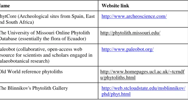
Comprehensive databases and atlases for phytolith identification do not exist yet. The web and scientific papers provide some atlases but the data are diverse, dispersed and not easily comparable. The data are presented generally by taxon (Family, Genus or Species) or by phytolith morphotypes. Modern phytolith assemblages have been extensively studied in Africa (Barboni et al., 2007). The PhytCore DB (http://www.phytcore.org) provides modern phytolith assemblages but it is very oriented for archeological studies. It is therefore important analysing modern soil or recent sediment samples in the surrounding vegetation types of the

25 “fossil” studied area. Here, we provide a non-exhaustive list of different phytolith atlases available on the web (Table 2).

Name Website link

PhytCore (Archeological sites from Spain, East and South Africa)

http://www.archeoscience.com/

The University of Missouri Online Phytolith Database (essentially the flora of Ecuador)

http://phytolith.missouri.edu/

Paleobot (collaborative, open-access web resource for scientists and scholars engaged in palaeobotanical research)

http://www.paleobot.org/

Old World reference phytoliths http://www.homepages.ucl.ac.uk/~tcrndf u/phytoliths.html

The Blinnikov's Phytolith Gallery http://web.stcloudstate.edu/msblinnikov/ phd/phyt.html

Table 2: List of phytolith atlases available online.

4. Terrestrial plant microfossils for qualitative and quantitative environmental reconstructions

4.1 Information from pollen

4.1.1 Environmental information

Fossil pollen assemblages are widely used for reconstructing past vegetation composition and distribution, and thereby climate and land-use changes. Pollen analysis is based on a set of principles that allow the pollen assemblage found in sedimentary archives to be related to the surrounding vegetation (e.g. Birks and Birks, 1980; Prentice, 1988). Information on the

26 pollen-vegetation relationship in particular is derived from the extensive study of surface (modern) pollen samples, taken in defined vegetation units characterizing an ecosystem or a bioclimate, as well as in various sedimentary contexts. Modern pollen rain-vegetation relationships were therefore investigated in a wide variety of landscapes worldwide, although some regions are still under-studied, such as arid and semiarid environments. From these studies arose several regional modern pollen databases for Europe (Davis et al., 2013; Fyfe et al., 2009), North America (Whitmore et al., 2005), East Asia (Zheng et al., 2014), Africa (Gajewski et al., 2002) and South America (Flantua et al., 2015).

Surface sample studies have shown there is no linear relationship between pollen proportions and plants abundances. Pollen proportions from a sedimentary archive give qualitative information on changes in vegetation composition through time and over a spatial area. Many studies demonstrated that pollen assemblages clearly discriminate between vegetation formations or forest-types and that pollen proportions of the major taxa reflect their relative importance in the vegetation (Prentice, 1988). Individual calibration studies prior to the analysis of a sedimentary archive are recommended to provide the characterization of the relationship between the pollen rain and local and regional vegetation essential to interpret the fossil pollen records in terms of vegetation changes. For example, in Southern Africa, Poaceae percentages were demonstrated to be critical to distinguish the pollen signal of the major biomes and associated climatic zones (Urrego et al., 2015). In the Mediterranean region, pollen assemblages within degraded maquis, for instance, appear largely influenced by adjacent land-covers such as conifer woodland and open vegetation (Gaceur et al., 2017). A large literature aims at understanding and estimating the factors that determine the source vegetation and modifies the pollen representativeness in terms of vegetation composition and abundance (e.g. Broström et al., 2008; Bunting et al., 2013; Gaillard et al., 2008; Havinga, 1984; Prentice, 1985; Sugita, 1994; Traverse, 2007). The differential pollen production,

27 dispersal and preservation between pollen taxa lead to the over- or under-representation of some morphotypes. The long-distance transport of anemophilous taxa is a common factor biasing the representation of the local vegetation by pollen assemblages (e.g. Traverse, 2007). This is particularly true in mountain regions where wind drives uphill transport of tree pollen (Ortu et al., 2006). The most widely known example is the over-representation of Pinus pollen that produces a large quantity of highly buoyant saccate pollen.

The structure and composition of the surrounding vegetation affect the source area of pollen. For instance, pollen rain in an open landscape is prone to increased contribution of pollen originating from distant vegetation (Bunting et al., 2004). The size (i.e. few meters to kilometers) and type (e.g. bogs, mires, lakes and ocean) of the sampling site also influence the pollen source area from local to regional inputs (e.g. Prentice, 1985; Sugita, 1994; Traverse, 2007). Ponds and small lakes mostly receive pollen from the vegetation surrounding the sampling site and therefore represent more local estimates of vegetation than large lakes (in their centers) that collect predominantly wind-transported pollen from the regional vegetation background (e.g. Sugita, 1994, 2007a, b). Note that without using specific pollen-based modelling approaches (see section 4.1.2) the dissociation between local and regional pollen signals cannot be assessed. Pollen studies on modern marine surface sediments showed that pollen assemblages reflect an integrated image of the regional vegetation of the adjacent continent (e.g. Heusser, 1983; Naughton et al., 2007). Such studies revealed that pollen grains are mainly transported to the ocean realm by wind and rivers but the role of these transport agents depends essentially on the environmental conditions of each area (e.g. Dupont et al., 2000; Groot and Groot, 1966). Pollen is predominantly supplied to the ocean by fluvial transport, in regions where hydrographic systems are well-developed such as in the western Iberian margin, northern Angola basin, western North Atlantic margin and in the Adriatic Sea (e.g. Bottema and van Straaten, 1966; Dupont and Wyputta, 2003; Heusser, 1983; Naughton

28 et al., 2007). In arid zones, such as northwest Africa, with weak hydrological systems and strong winds, pollen are mainly wind-blown (e.g. Hooghiemstra et al., 2006; Rossignol-Strick and Duzer, 1979). A mixture of fluvial and wind pollen transport may also occur as shown in the Gulf of Guinea (Lézine and Vergnaud-Grazzini, 1993) and the Alboran Sea (Moreno et al., 2002). Once in the ocean, pollen grains sink rapidly through the water column thanks to processes decreasing its buoyancy such as agglomeration (taking part to the marine snow), flocculation and incorporation in fecal pellets (Mudie and McCarthy, 2006) and thereby preventing long-distance transport by marine currents (Hooghiemstra et al., 1992).

4.1.2 Pollen-based land cover reconstruction

Pollen assemblages extracted from terrestrial sedimentary cores reflect a mix of both local and regional vegetation, and this makes difficult the assessment of quantitative vegetation

reconstruction based on pollen proportions. Correction factors were proposed as early as the fifties to minimize biases in the representativeness of pollen assemblages (see Birks and Berglund (2018) and references therein). From the eighties, important methodological

improvements took place with the development of models taking into account the differential production and dispersal of pollen, and the size and type of the sedimentary basin (e.g. Prentice and Parsons, 1983; Sugita, 1993, 1994, 2007a, b). These models have resulted in the development of the Landscape Reconstruction Algorithm (LRA, Sugita, 2007b) for

quantitative reconstruction of past vegetation composition.

The LRA approach corresponds to two sub-models, REVEALS (Regional Estimates of Vegetation Abundance for Large Sites, Sugita, 2007a) and LOVE (Local Vegetation Estimate, Sugita, 2007b). REVEALS reconstructs the regional vegetation composition in a radius of ca. 50 km using pollen counts from large lakes (>50 ha). REVEALS can also be

29 used for a combination of small and large lakes and bogs, although the standard errors would be greater than when using for a large lake only (Marquer et al., 2017; Trondman et al., 2016). LOVE reconstructs the local vegetation composition in a radius of few meters to kilometers that corresponds to the relevant source area of pollen (RSAP). To calculate quantitative estimates of local vegetation composition, LOVE uses pollen counts from small sites (lakes and bogs <50 ha) and subtracts the regional background of pollen using REVEALS

estimates(i.e. pollen coming from beyond the RSAP) . LOVE estimates represent the local vegetation composition within the RSAP. The LRA models incorporate critical parameters to correct the non-linear relationships between pollen percentages and plant abundances, e.g. pollen productivity estimates of specific plant taxa, fall speed of pollen and basin size, and several assumptions, e.g. specific wind speed and characteristics of atmospheric conditions. Current model improvements correspond to the implementation of an alternative pollen dispersal model in the LRA approach (e.g. Theuerkauf et al., 2016; Sugita, unpublished). The REVEALS and LOVE models are now increasingly applied to provide quantitative reconstructions of the Holocene vegetation composition from local, regional to sub-continental spatial scales (e.g. Cui et al., 2014; Fyfe et al., 2013; Hellman et al., 2008a; Hellman et al., 2008b; Marquer et al., 2017; Marquer et al., 2014; Mazier et al., 2015; Nielsen et al., 2012; Nielsen and Odgaard, 2010; Overballe‐Petersen et al., 2013; Soepboer et al., 2010; Sugita et al., 2010; Trondman et al., 2015; Trondman et al., 2016). The REVEALS model has largely been used for pollen-based land cover reconstruction in Europe and it is now applied to other regions (essentially in the northern hemisphere) via the support of the PAGES LandCover6k initiative (Gaillard et al., 2018). Evaluation of the LRA models reliability in the southern hemisphere and tropics (Southern Asia, Central Africa and South America) is in progress.

30 Contrary to the MAT method, the REVEALS approach requires some a priori information (i.e. explicit assumptions) on pollen productivity estimates (PPEs), lake size and wind speed. PPEs are difficult to estimate and time and resource consuming considering that taxon pollen productivity presents a high regional and interannual variability. Since all these parameters may vary through time, treating them as known processes increases the uncertainties of REVEALS land-cover reconstructions. However, REVEALS remains the only method that addresses these uncertainties directly, and at the taxon level. In addition, there are also subtle differences in the nature of the land-cover reconstruction between methods. For instance, REVEALS reconstructs the proportion of the land cover occupied by taxa in the landscape, irrespective of their physical size. In contrast, MAT methods often have a specific physical definition associated with the remote sensing datasets that are used for calibration, such as a minimum height (e.g. greater than 5 m) for forest taxa. This has implications in, for instance, shrub dominated landscapes such as forest-tundra landscapes where REVEALS may indicate more “forest” than MAT due to the low physical stature of the taxa (Zanon et al., 2018). An alternative and less resource intense approach has been developed by Williams (2003), based on the popular modern analogue technique (MAT) applied in pollen-climate

reconstructions, whereby analogues of fossil pollen samples are found in a modern pollen database. In the land-cover reconstruction method, the fossil sample is assigned to the remote-sensing derived forest cover of the closest matching modern pollen sample site.

This method is particularly useful to reconstruct past forest cover at continental scales. It was used to reconstruct Holocene forest cover in North America (Williams, 2003), Europe (Zanon et al., 2018), Northern Eurasia (Tarasov et al., 2007), and time slices for the whole of the northern hemisphere mid and high latitudes (Williams et al., 2011).

Zanon et al. (2018) showed that both methods generally provide comparable results.

31 offset reduces in some pioneer vegetation landscapes. This discrepancy may be due to

different definitions of ‘forest cover’ between the two methods, with trees greater than 5 m in the case of MAT, whereas forest is simply defined as the proportion of forest forming taxa irrespective of their size in REVEALS.

Other semi-quantitative methods for reconstructing land-cover are based on the ‘biomisation’ method (Prentice et al., 1996). This essentially compensates for differing pollen productivity and dispersion by transforming pollen percentages data using the square-root method. This has the effect of de-emphasising the taxa which represent the larger proportions (often the trees) and emphasizing more the taxa with the smaller proportions (often the herbaceous taxa). Taxa are then grouped according to common plant functional types (PFT’s) grouped in turn into biomes. The sum of the square rooted percentages of each group of taxa represents its ‘score’. The highest ‘score’ represents the vegetation biome of the pollen sample

assemblage. Biomisation classification schemes have been developed for almost all regions of the world (Prentice and Jolly, 2000). The original motivation for this work was the evaluation of climate model simulations through forward modelling. This side-steps the problems

associated with pollen-climate based data-model comparisons (see section 4.1.3) because the vegetation represented by the pollen record is directly compared with the vegetation generated by a process based vegetation model fed with output from the climate model simulation (Prentice et al., 1998). This approach has many advantages, not least the ability to take into account the complex response of vegetation to many different aspects of climate, such as temperature, precipitation, seasonality, cloudiness and frost frequency. Unfortunately, one of the main disadvantages is the difficulty in aligning the vegetation generated by the vegetation model with that represented by the pollen record. For instance, the link between the original biome vegetation model and pollen biomisation classification schemes (Prentice et al., 1996) is based on the unproven assumption that modelled Net Primary Productivity (NPP) is

32 directly linked to pollen percentages. Similarly, because the model generates potential natural vegetation, and the pollen data reflects actual vegetation, it becomes difficult to judge the accuracy of a pollen biomisation scheme with, for instance, over eight different schemes available in Europe alone (Allen et al., 2010; Allen et al., 2000; Bigelow et al., 2003; Binney et al., 2017; Marinova et al., 2018; Peyron et al., 1998; Prentice et al., 1996; Tarasov et al., 1998).

However, considering the simplicity of the approach, the biomisation procedure nevertheless proved to work remarkably well in many regions at continental scales. While the original procedure was developed specifically to reconstruct the natural potential vegetation, the procedure has also been adapted to reconstruct human impacted landscapes, the pseudo-biomisation approach (Fyfe et al., 2010). It was used to reconstruct the land-use and forest cover of Europe throughout the Holocene (Fyfe et al., 2015). Roberts et al. (2018) showed that the three methods, pseudo-biomisation, REVEALS and biomisation approaches, captured the basic trend in forest cover change over Europe during the Holocene.

Biomisation, pseudo-biomisation and modern analog technique can be used at continental and global scales and provide semi-quantitative estimates for biomes, plant functional types, land cover classes and tree covers, when LRA provides quantitative estimates of the cover of plant taxa at specific spatial scales, i.e. from local, regional to continental scales. Those quantitative estimates of vegetation are critical to i) evaluate climate and human-induced changes in vegetation composition and diversity, ii) answer archaeological questions about land use, iii) inform strategies related to conservation of natural resources and iv) be used as inputs for climate and dynamic vegetation modelling (e.g. Cui et al., 2014; Gaillard et al., 2010; Marquer et al., 2018; Marquer et al., 2017; Mazier et al., 2015).

33 Fossil pollen data have been used for quantitative reconstructions of past climate for over 70 years (Iversen, 1944). Pollen remains the main terrestrial proxy used for continental-scale evaluation of climate model simulations as part of the Paleo-climate Model Intercomparison Project (PMIP) for key time periods of the last climatic cycle (126, 21 and 6 ka) (Otto-Bliesner et al., 2017), and as far back as the mid-Pliocene (3.0-3.3 Ma) under the Pliocene Model Intercomparison Project (PlioMIP) (Haywood et al., 2013). Those models are used to simulate future climate and their palaeo-climate evaluations provide the only real test of reliability outside of our modern climatic experience. Palaeo-climate reconstructions have been based on widely spaced time-slices. It becomes possible now to produce spatially

explicit continuous reconstructions through time in data rich regions such as Europe (Davis et al., 2003b; Mauri et al., 2015) and North America (Viau and Gajewski, 2009). Spatially explicit reconstructions allow us to view the spatial structure of climate change, much of which is driven by change in atmospheric circulation which appears to be under-estimated in climate models (Mauri et al., 2014). The high spatial variability indicated by pollen synthesis studies (and others, see de Vernal and Hillaire-Marcel, 2006; Kaufman et al., 2004) suggests strong sampling bias in regional or even global interpretations from one or very few sites (Hansen et al., 2006; Marcott et al., 2013). Large networks of pollen sites allow area-average estimates that reflect more accurately climate system energy-balances. They are also more comparable with climate models with their large grid box resolutions (Bartlein et al., 2011). The main advantage of pollen data is its almost unrivalled spatial coverage from virtually all terrestrial regions of the Earth, together with the wide range of seasonal and annual climate parameters that can be commonly reconstructed. Disadvantages include relatively low centennial-scale temporal resolution (especially when multiple records are combined at large spatial scales), and the possibility that non-climatic environmental factors may also influence

34 the vegetation record through disease, succession, migration lag, soils and human action (Mauri et al., 2015). Another issue is the no-analogue-vegetation problem (Jackson and Overpeck, 2000; Williams et al., 2001), i.e. unique associations of taxa in the past that do not occur today, such as during the rapid post-glacial re-colonisation of higher mid-latitudes following the retreat of LGM ice sheets. This problem is also related to the no-analogue-climate problem, when there is no modern analogue for a no-analogue-climate in the past, such as the particular combination of seasonal insolation during the last Interglacial, or the low CO2

concentration during the LGM. It should be noted that the problem of human action on vegetation is often the inverse of how it is popularly conceived, since most transfer functions are assessed and calibrated for the present day when human action has probably been at its highest. It is in fact a lack of human action in the past that can create a no-modern-analogue problem for the transfer function.

Since the first pollen-climate transfer function over 70 years ago, there has been a large number of different methods developed, largely motivated by the problems that we have already outlined. These methods can be grouped into four main groups:

1) The first and generally the most popular group of methods is based on matching an assemblage of taxa present in a fossil pollen sample with unknown climate, with the same assemblage in a modern pollen sample whose climate is known. This includes the classic modern analogue technique (MAT), but also variants such as response surfaces (Brewer et al., 2007). Advantages include simplicity and an ability to incorporate non-linear responses to climate, while disadvantages include the need for a large calibration dataset of modern pollen samples and poor statistical treatment of uncertainties.

2) The second group of methods builds a regression model for each taxon based on the relationship between modern pollen samples and known modern climate, which is then used to deduct the past climate from the taxa in a fossil pollen sample assemblage. This includes

35 the popular Weighted Averaging – Partial Least Squares (WA-PLS) method (Birks et al. 2010). The advantage of this method includes better statistical treatment of uncertainties and elimination of problems such as spatial auto-correlation that are common to MAT. However disadvantages include heavy reliance on capturing the correct climate response within the calibration dataset and poor performance at the edges of the response envelope.

3) Both the previous two groups of methods require an extensive and representative modern pollen surface sample dataset for calibration of the transfer function, and also rely on the relative proportions of the taxa in the pollen assemblage. The third group of methods instead uses modern vegetation distribution rather than modern pollen samples as the basis for calibrating the transfer function, and generally uses presence and absence of taxa rather than its proportional occurrence in the assemblage. This includes classic methods such as mutual climatic range, as well as the more recent probability density function approach (Chevalier et al., 2014). These methods work by establishing the climate envelope for each taxon based on its modern vegetation distribution, and then combining the envelopes of the taxa found in the fossil pollen assemblage to deduce the most likely climate where all the taxa are able to exist together. This group of methods does not require a calibration dataset of modern pollen samples. They are especially good in areas where these datasets are limited such as in Africa (Chevalier et al., 2014), as well as being able to perform in no-analogue situations where taxa are found combined in assemblages that are not found today. The disadvantages of this type of model is that pollen may be found in areas beyond the geographical range of its source vegetation, while the use of geographical range alone to define the optimum climate for a taxa (rather than abundance) leads to large envelopes and consequently large uncertainties in reconstructions.

4) The final fourth group of methods uses a process based vegetation model to determine the climate of a fossil pollen assemblage. Normally vegetation models use climate data as input to

36 arrive at a vegetation, but in this ‘inverse’ method, the vegetation model is used in inverse mode where the vegetation is already known (the fossil pollen assemblage) and the most likely climate to result in that vegetation is the output. This method does not require any modern calibration data (although in reality vegetation models are largely parameterized based on what we know of modern vegetation), and since it is process based, it can provide reconstructions in no-analogue situations such as low CO2 climates (Wu et al., 2007).

The importance of pollen-based climate reconstructions are likely to increase in future as more climate models simulations are made in transient mode and at increasing spatial resolutions. At the same time, more fossil and modern calibration pollen data becomes available in public relational databases. Improvements in transfer function performance can also be expected, particularly through the application of Bayesian approaches that include multi-sample and multi-site analysis.

4.2 Information from microcharcoal

Vegetation fires produce different sizes of particles of which the smallest, classified as fine particles, are deposited far from the source (Patterson et al., 1987). Aeolian and fluvial processes are the main agent responsible for the transport of microcharcoal from the combustion site to the sedimentation basin where they are preserved. These microcharcoal particles remain in the atmosphere and are transported over long distances (Clark, 1988) by low atmospheric winds (<10 km) and deposited a few days or weeks after their formation (Clark and Hussey, 1996; Palmer and Northcutt, 1975). In water, after a short period of bedload transport, charred fragments break down into relatively resistant, somewhat rounded pieces, and thereafter remain stable. They exhibit the same behaviour as fragments of highly vesiculated pumice, which initially floats and then sinks as it becomes waterlogged (Nichols