HAL Id: insu-01351953
https://hal-insu.archives-ouvertes.fr/insu-01351953
Submitted on 10 Mar 2021HAL is a multi-disciplinary open access archive for the deposit and dissemination of sci-entific research documents, whether they are pub-lished or not. The documents may come from teaching and research institutions in France or abroad, or from public or private research centers.
L’archive ouverte pluridisciplinaire HAL, est destinée au dépôt et à la diffusion de documents scientifiques de niveau recherche, publiés ou non, émanant des établissements d’enseignement et de recherche français ou étrangers, des laboratoires publics ou privés.
Sokolovskiy
To cite this version:
Xavier J. Carton, Daniele Ciani, Jacques Verron, D Reinaud, Mikhail Sokolovskiy. Vortex merger in surface quasi-geostrophy. Geophysical and Astrophysical Fluid Dynamics, Taylor & Francis, 2015, 110 (1), pp.1 - 22. �10.1080/03091929.2015.1120865�. �insu-01351953�
January 2016, Volume 110 Issue 1 Pages 1-22
http://dx.doi.org/10.1080/03091929.2015.1120865 http://archimer.ifremer.fr/doc/00323/43460/
© 2016 Taylor & Francis
http://archimer.ifremer.fr
Vortex merger in surface quasi-geostrophy
Carton Xavier 1, *, Ciani Daniele 1, Verron J. 2, Reinaud J. 3, Sokolovskiy M. 41
Univ Bretagne Occidentale, LPO UMR6523, Brest, France.
2
Univ Grenoble 1, LGGE UMR5183, Grenoble, France.
3
Univ St Andrews, Sch Math & Stat, St Andrews, Fife, Scotland.
4
RAS, Lab Fluid Dynam, Inst Water Problems, Moscow 117901, Russia.
* Corresponding author : Xavier Cartonemail address : [email protected]
Abstract :
The merger of two identical surface temperature vortices is studied in the surface quasi-geostrophic model. The motivation for this study is the observation of the merger of submesoscale vortices in the ocean. Firstly, the interaction between two point vortices, in the absence or in the presence of an external deformation field, is investigated. The rotation rate of the vortices, their stationary positions and the stability of these positions are determined. Then, a numerical model provides the steady states of two finite-area, constant-temperature, vortices. Such states are less deformed than their counterparts in two-dimensional incompressible flows. Finally, numerical simulations of the nonlinear surface quasi-geostrophic equations are used to investigate the finite-time evolution of initially identical and symmetric, constant temperature vortices. The critical merger distance is obtained and the deformation of the vortices before or after merger is determined. The addition of external deformation is shown to favor or to oppose merger depending on the orientation of the vortex pair with respect to the strain axes. An explanation for this observation is proposed. Conclusions are drawn towards an application of this study to oceanic vortices.
Keywords : shear/strain flow, steady states, vortex merger, numerical model, Surface
For Peer Review Only
1
Introduction
The intrinsic or forced instabilities of ocean currents and the turbulent atmospheric forcing generate energetic motions at the mesoscale in the ocean; these motions have horizontal scales of 20 to 200 km and advective timescales of a few days to a few weeks (though the lifetime of these motions can range from a few months to sometimes years). These mesoscale motions are often composed of vortices (horizontally recirculating motions) but also of meanders and waves, and the whole oceanic mesoscale circulation is at least as energetic as (and often more energetic than) the large scale circulation (Zhang et al., 2014).
Once formed, vortices in the ocean can interact if they are locally numerous enough or close enough. This occurs for instance for Gulf Stream rings, or for Mediterranean Water eddies near the Iberian coast (Carton et al., 2010; L’Hegaret et al., 2014). These Mediter-ranean water eddies were shown to interact as a result of their advection by cyclonic partner vortices. Such collisions of baroclinic cyclone-anticyclone vortex pairs (called ”hetons”) have been widely studied in the literature, and shown to be efficient to lead to the merger of two vortices (see for instance Sokolovskiy and Verron, 2000a,b; Sokolovskiy and Carton, 2010). When two like-signed vortices come in close contact, they can merge to form a vortex which is often larger. Vortex merger has been studied in two-dimensional or quasi-geostrophic mod-els, relevant to the mesoscale dynamics in the ocean interior (Overman and Zabusky, 1982; Dritschel, 1985, 1986; Griffiths and Hopfinger, 1987: Melander et al., 1987, 1988; Pavia and Cushman-Roisin, 1990; Carnevale et al. 1991; Carton, 1992; Bertrand and Carton, 1993; Valcke and Verron, 1993; Verron and Valcke, 1994; Yasuda, 1995; Yasuda and Flierl, 1995; Valcke and Verron, 1996, 1997; Yasuda and Flierl, 1997; von Hardenberg et al., 2000; Dritschel, 2002; Reinaud and Dritschel, 2002; Meunier et al., 2002; Bambrey et al. 2007; Ozugurlu et al., 2008). Depending on the initial conditions, the merging process can finally form one large vortex or two asymmetric vortices. Vortex merger also produces smaller scale features such as small eddies and filaments. These smaller features compose (in part) the oceanic submesoscale. It has recently been shown that submesoscale eddies can also merge and thus form mesoscale vortices (Barbosa Aguiar et al., 2013).
A simple model apt to represent the oceanic submesoscale is the surface quasi-geostrophy (hereafter SQG). In particular, it is able to represent the dynamics of thermal fronts at the ocean surface (such fronts are observed daily in the coastal zone for instance, or near intense jets such as the Gulf Stream). Associated with these fronts are intense upward and down-ward velocities, which have been proved to be better represented by SQG dynamics than by 3D QG models (Klein and Lapeyre, 2009). Based on this property, an ”effective” SQG method was designed to reconstruct low-frequency, 3D motions, above the thermocline using high-resolution surface data only (Klein et al., 2009).
Indeed, though the SQG model was originally designed to study the atmospheric motions at the tropopause (Blumen, 1978; Juckes, 1994; Held et al., 1995), it has been used later to investigate oceanic submesoscale dynamics, essentially from the point of view of turbulence (Lapeyre and Klein, 2006). The energy spectra in SQG simulations of turbulence are close
3 4 5 6 7 8 9 10 11 12 13 14 15 16 17 18 19 20 21 22 23 24 25 26 27 28 29 30 31 32 33 34 35 36 37 38 39 40 41 42 43 44 45 46 47 48 49 50 51 52 53 54 55 56
For Peer Review Only
to those of primitive equation1 simulations, but noticeably different from those of 3D QG turbulence. One limitation of SQG models for ocean turbulence simulations, though, is the absence of ageostrophic processes able to transfer energy to small scales (Capet et al., 2008). Nevertheless, SQG models have proven their ability to represent fairly accurately complex real situations.
A few studies of single vortex or of vortex pair dynamics have been conducted in SQG, often concentrating on vortex stability (Juckes, 1995; Muraki and Snyder, 2007; Carton, 2009; Harvey and Ambaum, 2010, 2011; Harvey et al., 2011). Like signed vortex interaction at different levels (the so-called vortex alignment) was studied in a 3D quasi-geostrophic model coupled to SQG dynamics (Perrot et al., 2010).
To assess the importance of vortex merger for the growth of submesoscale eddies, we inves-tigate here the merger of two patches of surface temperature in the SQG model.
The outline of the paper is the following. We will first recall the SQG model and physical configuration, we will briefly analyse the deformation of two finite-area vortices in a co-rotating configuration. Then, using numerical simulations of a SQG model, we will survey the nonlinear regimes for two such interacting vortices and analyse these regimes. Finally, conclusions will be provided.
2
Model and parameters
Surface quasi-geostrophy is the geostrophic dynamics of potential temperature anomalies at the surface of a stratified, rotating fluid with zero internal potential vorticity.
When the buoyancy frequency is constant, N2(z′
) = N2
0, the vertical coordinate can be
rescaled as z = N0z′/f0 where z′ is the physical vertical coordinate; potential vorticity is
then
Q = 0 = [∂x2 + ∂2y + ∂z2]ψ where ψ(x, y, z, t) is the streamfunction.
At the surface of the fluid, potential temperature is related to streamfunction in dimen-sionless form, via θ(x, y, t) = ∂zψ(x, y, z = 0, t) (the normalization of all variables is given
in Muraki et al., 1999). Potential temperature is advected by the horizontal velocity at the surface according to
∂tθ + J(ψ(z = 0), θ) = 0 (1)
with u = −∂yψ(z = 0), v = ∂xψ(z = 0).
Note that this equation can be generalized to accomodate an external (strain or rotation) field, or a mean temperature gradient
∂tθ + J(ψ(z = 0) + ¯ψ(x, y, z = 0), θ + ¯θ(y)) = 0 (2)
1
Primitive equations are Boussinesq, hydrostatic Navier-Stokes equations on a rotating planet
3 4 5 6 7 8 9 10 11 12 13 14 15 16 17 18 19 20 21 22 23 24 25 26 27 28 29 30 31 32 33 34 35 36 37 38 39 40 41 42 43 44 45 46 47 48 49 50 51 52 53 54 55 56
For Peer Review Only
For instance, ¯ψ(x, y, z = 0) = (Ω/2) (x2 + y2) − (S/2) (x2 − y2) or ¯θ(y) = ¯θy/L, where Ω the rotation rate and S is the strain rate. In this paper, we will assume that there is no mean temperature gradient ¯θ.
Since potential vorticity is null in the fluid interior, a relation holds between temperature and streamfunction in spectral space
ˆ
ψ(k, l, z, t) = 1
Kθ(k, l, t)eˆ
Kz
where k and l are the zonal and meridional wavenumbers, and K =√k2+ l2. The positive
exponent in the term eKz is related to the application to the ocean where z < 0 (the surface
lies at z = 0); for atmospheric applications, this term should be e−Kz
(for z > 0).
3
Analytical theory of co-rotating surface vortices
3.1
Point vortex approach: co-rotation and steady states
The motion of two surface point vortices, possibly in an external deformation field, is driven by their mutual influence and by the external velocity field (see figure 1). Calling S the external strain rate, and Ω the external rotation, the total streamfunction is at point (x, y) in the plane, ψ(x, y) = ψv(x, y) + S 2 (y 2 − x2) + Ω 2 (x 2+ y2).
Using polar coordinates (r, φ), the streamfunction reads
ψ(r, φ) = ψv(r, φ) −
Sr2cos(2φ)
2 +
Ωr2
2 .
We call (rp(t), φp(t)) and (rp(t), φp(t)+π) the instantaneous vortex positions (see again figure
1). Both vortices have the same strength (equal to the surface integral of temperature, if the vortices had a finite area)
κ = Z Z
θdxdy
Initially (and thus at all times), the point vortices and the external field are symmetric with respect to the center of the domain. Therefore, we can study the motion of one vortex only.
The streamfunction created by these point vortices can be calculated from their temperature distribution (a sum of Dirac’s delta functions) via a convolution with a Green’s function. The Green’s function for SQG vortices is G(r′
) = 1/(2πr′
) so that
ψv(r, φ) = κ/(2πd1) + κ/(2πd2)
with d2
1 = r2+ r2p− 2rrpcos(φ − φp) and d22 = r2+ r2p+ 2rrpcos(φ − φp).
3 4 5 6 7 8 9 10 11 12 13 14 15 16 17 18 19 20 21 22 23 24 25 26 27 28 29 30 31 32 33 34 35 36 37 38 39 40 41 42 43 44 45 46 47 48 49 50 51 52 53 54 55 56
For Peer Review Only
Figure 1: Sketch of the two surface temperature point vortices in the external strain and rotation fields. 3 4 5 6 7 8 9 10 11 12 13 14 15 16 17 18 19 20 21 22 23 24 25 26 27 28 29 30 31 32 33 34 35 36 37 38 39 40 41 42 43 44 45 46 47 48 49 50 51 52 53 54 55 56
For Peer Review Only
Knowing that no point vortex induces velocity on itself, we can use the formula above to calculate the motion of the point vortex in (rp, (t)φp(t)). The equations for the radial and
orthoradial velocities, are
vr(rp, φp) = ˙rp(t) = − 1 r ∂ψ ∂φ|r=rp(t),φ=φp(t) = − Srpsin(2φp) (3a) vφ(rp, φp) = rp(t) ˙φp(t) = ∂ψ ∂r′|r=rp(t),φ=φp(t) = −κ 8πr2 p + rpΩ − Srpcos(2φp) (3b)
where ˙X denotes the time derivative of X.
For these equations, we have two sets of steady solutions: 1) If S = 0, then r3
p = κ/(8πΩ) is a solution for all φp if this ratio is finite, and positive.
2) If S 6= 0, then sin(2φp) = 0 (the solution rp = 0 is physically excluded), which leads to a
discrete number of solutions φp = ‘φn = nπ/2, (n = 0, 1). Then, the corresponding radius
for steady evolution is given by
rp3 = r3n= κ
8π(Ω + (−1)n+1S)
if S 6= ±Ω and if this ratio is positive.
We linearize the equations of motion around the equilibria and investigate the fate of in-finitesimal disturbances r′
in radius and φ′
in angle.
If S = 0, then the perturbation in radius is invariant and the perturbation in angle varies linearly. If S 6= 0, the equations are
˙r′ = (−1)n+1 2Srn φ′ ˙ φ′ = 3κr ′ 8πr4 n
The stability analysis proceeds by combining these two equations into one for r′
(or for φ′ ) which reads ¨ r′ + Ar′ = 0 where A = 3(−1)4πrn3Sκ
n . If A > 0 then the configuration is stable. For n = 0, this implies that
κ · S be positive and conversely for n = 1.
In the 2D Euler dynamics, the equations are very similar, but the Green’s function is ln(r)/(2π) and vorticity replaces temperature anomaly. In 2D dynamics, the stability of two point vortices in a stationary external flow, is governed by the value of A = (−1)πrn+12 Γ·S
n
, where Γ is the circulation (area integral of relative vorticity) in 2D incompressible dynamics (Perrot and Carton, 2010).
In this case, for stability, Γ · S has to be negative for n = 0 and conversely for n = 1. Physically, this is identical to the SQG result. Indeed, positive vorticity corresponds to negative temperature anomaly, so that κ has an opposite sign to Γ.
3 4 5 6 7 8 9 10 11 12 13 14 15 16 17 18 19 20 21 22 23 24 25 26 27 28 29 30 31 32 33 34 35 36 37 38 39 40 41 42 43 44 45 46 47 48 49 50 51 52 53 54 55 56
For Peer Review Only
Figure 2: Sketch of the finite-area surface temperature vortex under the influence of a distant point (temperature) vortex.
3.2
Analytical theory of the mutual deformation of finite-area
sur-face temperature vortices
Next, we study the evolution of two like-signed, finite core vortices. First, we consider the vortex pair in the absence of external strain. In this case the two vortices rotate around the origin. Each vortex can be deformed by its companion’s sheared velocity field.
If the separation distance between the two vortices is large, the shear induced by a vortex (of radius R and of uniform temperature θ0) onto another can be represented asymptotically
by that induced by a singularity placed at its centre and of same strength κ = πR2θ 0 (see
figure 2). The point vortex is located at a distance d from the patch (or finite-area vortex) and we assume that R/d = ǫ ≪ 1.
The streamfunction created by the distant point vortex on the finite-area vortex, at any point (r, φ) in the reference frame relative to C2 (see figure 2), is
ψ = κ/(2πs) = κ
2πd (1 + 2(r/d) cos(φ) + r
2/d2)(−1/2)
From this expression of streamfunction, one can compute the radial and orthoradial velocities
3 4 5 6 7 8 9 10 11 12 13 14 15 16 17 18 19 20 21 22 23 24 25 26 27 28 29 30 31 32 33 34 35 36 37 38 39 40 41 42 43 44 45 46 47 48 49 50 51 52 53 54 55 56
For Peer Review Only
in the same framework
upvr = κ sin(φ) 2πd2 (1 + 2(r/d) cos(φ) + r 2/d2)(−3/2) (1 + 4(r/d) cos(φ) + 4(r/d)2)1/2 upvφ = −κ[cos(φ) + r/d] 2πd2 (1 + 2(r/d) cos(φ) + r 2/d2)(−3/2)
Note that C2 rotates around O at the rate
Ω2 = −ǫ2θ0/d = −κ/(πd3)
In the expressions for the velocity, we now set r = R and use a Taylor expansion in ǫ to find
upvr = θ0 2 (ǫ 2 sin(φ) −1 2ǫ 3 sin(2φ))
The mode 1 component (in sin(φ)) corresponds to a displacement. Thus we will compute the effect of the mode 2 component which leads to an elliptical deformation of the finite-area vortex.
To find the finite-area vortex contour deformation, one can use the kinematic equation for the vortex boundary. This equation decribes the motion of any point on this contour in the rotating frame of reference. The kinematic equation is
∂tη + (uφ/R) ∂φη = ur+ upvr
where ur is the radial velocity of the finite-area vortex, due to its contour perturbation η.
It can be computed following the formulae provided in Harvey and Ambaum (2010). We can also replace ∂tη = −Ω∂φη and expand the contour perturbation in Fourier modes of the
angle
η =X
n
ηnexp(inφ).
The kinematic equation can be reordered as
−Ω∂φη − upvr = limr→R(ur− (uφ/R) ∂φη)
From this, and setting n = 2, one can find the amplitude of the elliptical deformation of the contour η2 via
−2iΩη2 + (i/4) θ0ǫ3 = (2iθ0/R) η2 limr→R[E2(r/R) − E1(r/R)]
where
En(r/R) =
Z ∞ 0
Jn(k)Jn(kr/R)dk
(see Harvey et al., 2011), and Jnis the Bessel function of the first kind and of order n. Using
limr→R[E2(r/R) − E1(r/R)] = −2/(3π) (see again Harvey et al., 2011), we obtain
η2 R = −3πǫ3 16(1 + 3πǫ3/4) 3 4 5 6 7 8 9 10 11 12 13 14 15 16 17 18 19 20 21 22 23 24 25 26 27 28 29 30 31 32 33 34 35 36 37 38 39 40 41 42 43 44 45 46 47 48 49 50 51 52 53 54 55 56
For Peer Review Only
a) -0.4 -0.3 -0.2 -0.1 0 0.1 0.2 0.3 0.4 -1 -0.5 0 0.5 1 y xCo-rotating vortex steady states, SQG
’vortex contour’ b) -0.4 -0.3 -0.2 -0.1 0 0.1 0.2 0.3 0.4 -1 -0.5 0 0.5 1 y x
Co-rotating vortex steady states, SQG (with strain)
’vortex contour’
Figure 3: Steady states of two co-rotating surface temperature vortices, for decreasing inner abscissa, (a) in the absence of external flow, (b) with a pure strain S = 0.5. The vortices are confined between x = a and x = 1; for both cases (without or with external flow), the steady states for a = 0.9, 0.75, 0.6, 0.45, 0.3, 0.15, 0.1, 0.05, 0.025 are superimposed (hence the presence of 9 different contours).
3 4 5 6 7 8 9 10 11 12 13 14 15 16 17 18 19 20 21 22 23 24 25 26 27 28 29 30 31 32 33 34 35 36 37 38 39 40 41 42 43 44 45 46 47 48 49 50 51 52 53 54 55 56
For Peer Review Only
Therefore, the elliptical deformation of the vortices varies as (R/d)3 at large distances. Note that this deformation is weaker than that due to a companion vortex in 2D incompressible flows, which varies as (R/d)2 at large distances. Note also that this asymptotic theory cannot
predict deformations for close vortices, hence close co-rotating steady states. To determine these steady states, we resort to a numerical procedure.
3.3
Numerical determination of steady states of two co-rotating,
finite area, surface temperature vortices
The steady states of two co-rotating surface vortices are determined using an iterative method. The first guess for the vortex contour is either circular, or the stretched previ-ous equilibrium. The vortex boundary is confined between x = a and x = 1. The value of a is decreased from one case to the next. The method uses the Overman- Zabusky (1982) desingularized procedure.
It is implemented firstly in the absence of external deformation field. The steady vortex con-tours are shown on figure 3, for decreasing values of the innermost edge a of the vortex. In an equivalent manner, this corresponds to a decreasing distance between the vortex centers. The various steady states (for various values of a) are superimposed to show the increas-ing deformation of the contours as the vortices get closer. As anticipated by the analytical calculation above, the first and dominant deformation of the vortices is the elliptical mode (azimuthal mode 2; see figure 3a). Higher modes (like the triangular mode 3) set in when the vortices are very close.
In the presence of an external deformation field (here a strain field), the steady states are more elongated along the Ox direction (more squeezed in the transverse direction), and more elliptical, as expected for a deformation field varying quadratically with x and y (see figure 3b).
4
Nonlinear regimes of two interacting surface
vor-tices, and their analysis
A numerical model of the SQG equations is used here. This model is based on a projec-tion/truncation of the equations on Fourier modes (implying periodicity in both horizontal directions). The domain size is 2π×2π with 256 or 512 grid points in each direction. Minimal biharmonic viscosity is used to remove spurious features, resulting from enstrophy accumu-lation, at small scales: equation (1) is integrated with a right-hand side equal to ν4∇4hθ. In
dimensionless terms, biharmonic viscosity is ν4 = 10−9 for the 512 x 512 resolution.
The initial condition consists of two patches of uniform potential temperature θ0, of radius
R (R = 0.5 in the numerical model), and lying at a distance d. In the numerical model, the edges of the vortices are slightly smoothed to avoid the numerical instability (Gibbs’ effect)
3 4 5 6 7 8 9 10 11 12 13 14 15 16 17 18 19 20 21 22 23 24 25 26 27 28 29 30 31 32 33 34 35 36 37 38 39 40 41 42 43 44 45 46 47 48 49 50 51 52 53 54 55 56
For Peer Review Only
associated with a discontinuity of temperature anomaly.
4.1
Two-vortex evolution in the absence of external flow
Here, the pseudo-spectral code of the SQG equations is run for two symmetric, initially cir-cular vortices (with radius R). The initial distance d between the vortex centers is varied. We note that the self-rotation period, or turn-over period, of a vortex is Tv = 2π (in model
time units). The nonlinear evolution of the vortices is described and analysed. We recall that in 2D (incompressible) dynamics, the critical distance below which the two eddies merge is about d = (3.25 ± 0.05) R. For 3D QG vortex merger (with vortices at the same depth), the critical merger distance is d = 2.55R (for complete merger; it is d = 2.6R for partial merger; see Reinaud and Dritschel, 2005, figure 24).
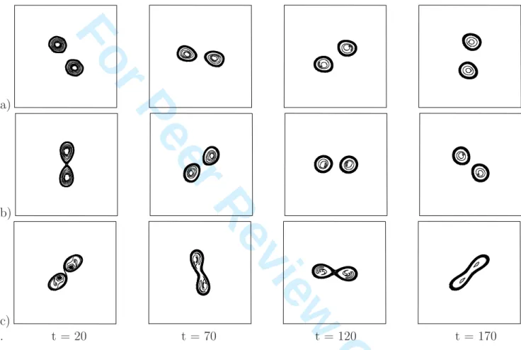
In the absence of external deformation field, the SQG evolutions are the following: For d/R = 3.5, the two vortices wobble in co-rotation around the center. Their mutual influence results in a mode 2 and a mode 4 deformation on their contours. No filamentation occurs (see figure 4a). This is an elastic interaction (see Dritschel, 2002 or Reinaud and Drischel, 2002).
For d/R = 3.2, the two vortices oscillate in co-rotation, do not touch each other, and adopt a mostly elliptical shape. Again, this is an elastic interaction.
For d/R = 3.1, the two vortices co-rotate but can temporarily touch at the center of the plane; once separated they develop elliptical and asymmetric deformations (see figure 4b). This evolution can be characterized as a weak exchange.
For d/R = 3.0, the two vortices join at the center, then separate, and this process is repeated at least four times during the stage of non-viscous evolution. The vortices form a rotating figure 8 structure (see figure 4c).
The time evolution of two steady states (with a = 0.1 and with a = 0.025) in the spectral code, is shown in appendix. In general, the time evolutions of steady states show vacillations; these perturbations can be related to the initial interpolation and smoothing of the steady states in the spectral code2.
We can note (visually) that the evolution of the vortex pair with d/R = 3.1 presents some similarity with the evolution of the steady state with a = 0.1; to a lesser degree, the evolution of the vortex pair with d/R = 3.0 resembles that of the steady state with a = 0.025.
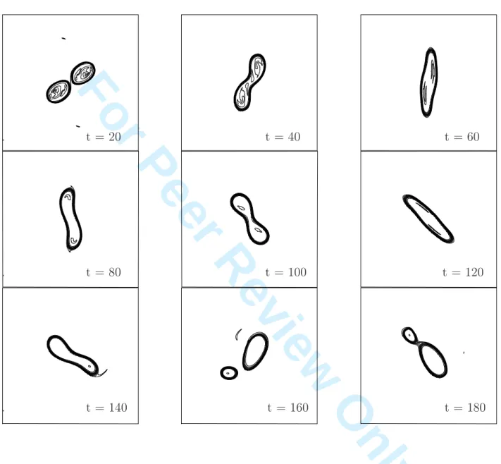
For d/R = 2.9, the two vortices merge, separate and then irreversibly merge to form a vortex with a strong contour deformation, mainly on modes 2 and 4. After a long adjust-ment period of this merged vortex, asymmetric modes (1 and 3) grow, forming a cusp on the vortex contour. This asymmetry amplifies to split the vortex into two vortices of different sizes which finally interact again (see figure 5). This evolution is a partial merger.
For d/R = 2.8, the two vortices merge immediately and irreversibly; they eject filaments
2
As mentioned above, smoothing is necessary to avoid the Gibbs’ numerical instability
3 4 5 6 7 8 9 10 11 12 13 14 15 16 17 18 19 20 21 22 23 24 25 26 27 28 29 30 31 32 33 34 35 36 37 38 39 40 41 42 43 44 45 46 47 48 49 50 51 52 53 54 55 56
For Peer Review Only
a)
b)
c)
. t = 20 t = 70 t = 120 t = 170
Figure 4: Time evolution of two surface temperature vortices for row (a) d/R = 3.5; row (b) d/R = 3.1; row (c) d/R = 3.0 initially. Temperature contour interval is 0.1 (from zero to unity). Frames are shown every fifty model time units (starting at 20 model time units, and advancing from left to right). We recall that the self-rotation period of a single vortex is Tv = 2π model time units.
3 4 5 6 7 8 9 10 11 12 13 14 15 16 17 18 19 20 21 22 23 24 25 26 27 28 29 30 31 32 33 34 35 36 37 38 39 40 41 42 43 44 45 46 47 48 49 50 51 52 53 54 55 56
For Peer Review Only
. t = 20 t = 40 t = 60
. t = 80 t = 100 t = 120
. t = 140 t = 160 t = 180
Figure 5: Time evolution of the surface temperature vortices for d/R = 2.9 initially (time advancing from left to right, then from top to bottom); temperature contour interval is 0.1 (from zero to unity). Frames are shown every twenty model time units (starting at 20 model time units). The self-rotation period of a vortex is Tv = 2π model time units.
3 4 5 6 7 8 9 10 11 12 13 14 15 16 17 18 19 20 21 22 23 24 25 26 27 28 29 30 31 32 33 34 35 36 37 38 39 40 41 42 43 44 45 46 47 48 49 50 51 52 53 54 55 56
For Peer Review Only
a)
b)
. t = 5 t = 35 t = 65 t = 95
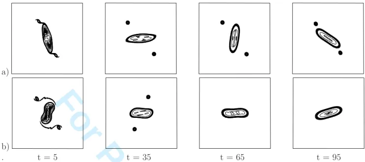
Figure 6: Time evolution of the surface temperature vortices for (a) d/R = 2.8, (b) d/R = 2.5 initially. Time advances from left to right. Temperature contour interval is 0.1 (from zero to unity). Frames are shown every thirty model time units (starting at 5 model time units). We recall that the self-rotation period of a single vortex is Tv = 2π model time units.
which roll up into peripheral vortices. The final central vortex is elliptical with a superim-posed, oscillatory mode 4 deformation; it remains very elongated (see figure 6a). Again, this evolution is a partial merger.
For d/R = 2.5, the same process occurs, but the peripheral vortices are finally absorbed by the central vortex; the final state of this vortex is elliptical (mode 4 is weak); it is less elongated than for d/R = 2.8, but it does not axisymmetrize (see figure 6b). This evolution is a complete merger.
Four main conclusions can be drawn from these simulations:
1) the regime separation between co-rotation and merger is less clear cut than for 2D incom-pressible flows. But the final asymmetric evolution observed for d/R = 2.9 is characteristic of partial merger, often achieved in QG vortex merger.
2) Near the merging threshold (in d/R), asymmetric (and high) modes of deformation de-velop on each vortex. They correspond to the tip, or cusp, near the center of the plane. Merger starts when the two vortices get in contact, on the side of this tip.
3) The critical merger distance for SQG vortices is smaller than for their 2D counterparts. Considering the d/R = 3.0 and d/R = 2.9 cases as marginal, the merger process without further breaking is observed only for d/R = 2.8 which is noticeably below the 3.2 − 3.3 value for 2D vortices. This is attributed to the shorter ranged Green’s function in SQG dynamics. 4) In SQG dynamics, filaments more easily roll up into small eddies than in 2D dynamics (as previously observed).
3 4 5 6 7 8 9 10 11 12 13 14 15 16 17 18 19 20 21 22 23 24 25 26 27 28 29 30 31 32 33 34 35 36 37 38 39 40 41 42 43 44 45 46 47 48 49 50 51 52 53 54 55 56
For Peer Review Only
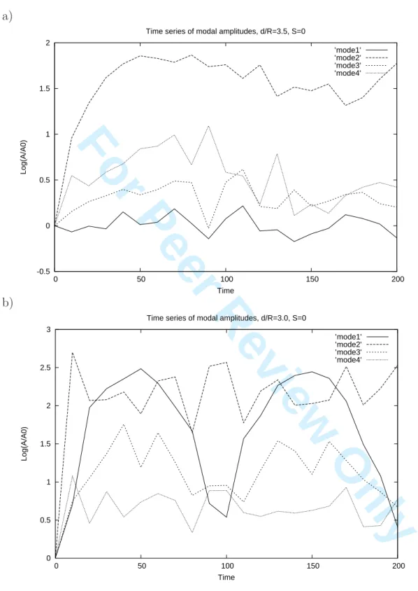
To support remark (2), we performed a Fourier analysis of the deformation of the co-rotating vortex contours for d/R = 3.5 and for d/R = 3.1. The initial circular state of the vortices was substracted from the instantaneous state in the co-rotating frame of reference and the disturbance was decomposed into azimuthal modes 1 to 4. The amplitude of the modes of deformation on the vortex contours, versus time, is shown on figure 7a-b.
In the case d/R = 3.5, mode 2 (of contour deformation) grows the most and the fastest, followed by mode 4 which is fed by the self interaction of mode 2 (see figure 7a). The asymmetric modes remain weaker. Nevertheless, the final state is not axisymmetric. Fur-thermore, viscosity is kept to a minimum which thus prevents a fast damping of smaller-scale perturbations.
In the case d/R = 3.0, more deformation of the vortices is observed and in particular the asymmetric modes are stronger than in the previous case, and stronger than mode 4 (see figure 7b). This corresponds to the rotating figure-8 structure. In this structure, each vortex contour is deformed on modes 2 and 3. The periodic growth and decay of mode 1 correspond to the radial motion of the vortices towards the center of the plane and to their further re-traction.
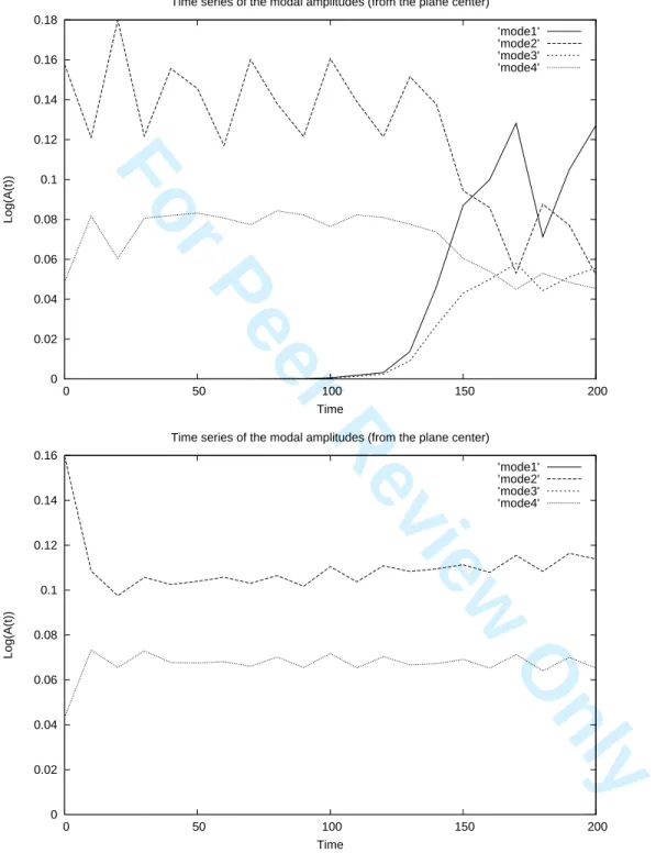
The following analysis quantifies the modal components of the flow, now computed from the center of the plane. This analysis focuses therefore more on the final product of the flow, the merged vortex, but it is also able to characterize a flow asymmetry during the unsteady evolution. The results are shown on figure 8 for d/R = 2.9 and for d/R = 2.8.
Clearly, in the first case, many asymmetric modes grow after about 100 model time units, corresponding to the breaking up of the merged vortex into two asymmetric fragments. On the contrary, only modes 2 and 4 are present in the second case, both during vortex merger and during the pulsation of the merged vortex.
These analyses clearly indicate the importance of the asymmetric modes near the threshold for merger (in vortex separation). Away from this threshold, the vortex oscillation and co-rotation, or merger and further pulsation imply mostly the elliptical and square modes of deformation.
4.2
Vortex pair evolution in the presence of external deformation
The global rotation Ω is chosen positive and equal to |2S|. The strain S can be positive or negative. This choice is motivated by the existence of equilibria for the equivalent point vortices; it is also motivated by a similar choice for the study of 2D vortex merger in the presence of strain and rotation (Perrot and Carton, 2010).
The vortex centers are initially located along the x-axis. Point vortex theory states that, under such conditions, there are two possible steady states (along the x-axis or along the y-axis). The vortex pair is oriented initially along the x-axis (note that orienting them along the y-axis will give the same results if the sign of the strain is changed).
A series of simulations with the nonlinear model is conducted in the presence of shear
3 4 5 6 7 8 9 10 11 12 13 14 15 16 17 18 19 20 21 22 23 24 25 26 27 28 29 30 31 32 33 34 35 36 37 38 39 40 41 42 43 44 45 46 47 48 49 50 51 52 53 54 55 56
For Peer Review Only
a) -0.5 0 0.5 1 1.5 2 0 50 100 150 200 Log(A/A0) TimeTime series of modal amplitudes, d/R=3.5, S=0
’mode1’ ’mode2’ ’mode3’ ’mode4’ b) 0 0.5 1 1.5 2 2.5 3 0 50 100 150 200 Log(A/A0) Time
Time series of modal amplitudes, d/R=3.0, S=0
’mode1’ ’mode2’ ’mode3’ ’mode4’
Figure 7: Time evolution of the modal disturbance (modes 1 to 4) on the vortex contours for (a) d/R = 3.5 and (b) d/R = 3.1 initially. The modal amplitudes are normalized by their initial value and are plotted in semilog scale.
3 4 5 6 7 8 9 10 11 12 13 14 15 16 17 18 19 20 21 22 23 24 25 26 27 28 29 30 31 32 33 34 35 36 37 38 39 40 41 42 43 44 45 46 47 48 49 50 51 52 53 54 55 56
For Peer Review Only
0 0.02 0.04 0.06 0.08 0.1 0.12 0.14 0.16 0.18 0 50 100 150 200 Log(A(t)) TimeTime series of the modal amplitudes (from the plane center) ’mode1’ ’mode2’ ’mode3’ ’mode4’ 0 0.02 0.04 0.06 0.08 0.1 0.12 0.14 0.16 0 50 100 150 200 Log(A(t)) Time
Time series of the modal amplitudes (from the plane center) ’mode1’ ’mode2’ ’mode3’ ’mode4’
Figure 8: Time evolution of the modal disturbance (modes 1 to 4) computed from the center of the plane for d/R = 2.9 (top) and d/R = 2.8 (bottom) initially.
3 4 5 6 7 8 9 10 11 12 13 14 15 16 17 18 19 20 21 22 23 24 25 26 27 28 29 30 31 32 33 34 35 36 37 38 39 40 41 42 43 44 45 46 47 48 49 50 51 52 53 54 55 56
For Peer Review Only
d/R
2s
0.01 0.02 0.03 0.04 0.05
0
−0.01
−0.02
−0.03
−0.04
−0.05
2.4
3.0
2.8
2.6
3.2
3.4
3.6
3.8
4.0
4.2
4.4
4.6
AS
AS
CR
CR
CR CR
CR
M
M
CR
DC
CR
CR
CR
DC
MA
M
MA
DC
DC
DC
CR CR
MA
MA
MA
MA
MA
M
M
MA
MA
DC
DC
DC
DC
DC
DC
DC
DVM
M
DVM
DVM
DC
AS
MA
MA
MA
MA
MA
MA
M
MA
MA
MA
MA
MA
MA
MA
MA
MA
DC
MA
MA
DVM
OS
OS
DC
OS
OS
OS
OS
OS
OS
OS
OS
OS
OS
DC
OS
DVM
DVM DC
DVM DC
MA
MA
CR
M
Figure 9: Regime diagram in the (2s, d/R) plane with Ω = |2s| obtained from nonlinear simulations of two vortex evolution. M denotes vortex merger, MA denotes vortex merger with final asymmetry, CR denotes co-rotation, AS indicates asymmetric evolution into a large vortex and a smaller one, after merger, OS denotes vortex oscillation around the steady states, DC denotes an alternation of divergence and convergence of the vortices; finally, DVM represents an initial divergence of the vortices followed by a convergence and merger.
3 4 5 6 7 8 9 10 11 12 13 14 15 16 17 18 19 20 21 22 23 24 25 26 27 28 29 30 31 32 33 34 35 36 37 38 39 40 41 42 43 44 45 46 47 48 49 50 51 52 53 54 55 56
For Peer Review Only
a)
b)
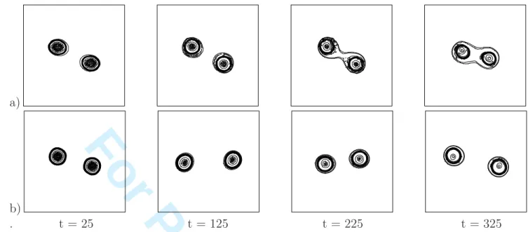
. t = 25 t = 125 t = 225 t = 325
Figure 10: Time evolution of the surface temperature vortices for (a) d/R = 3.0, Ω = 2S = 0.05 (OS regime); (b) d/R = 4.2, Ω = 2S = 0.02 (DC regime). Time advances from left to right. Temperature contour interval is 0.1 (from zero to unity). Frames are shown every hundred model time units (starting at 25 model time units). We recall that the self-rotation period of a single vortex is Tv = 2π model time units.
and strain. Seven main regimes are observed : (1) symmetric merger, (2) merger followed by a (weakly) asymmetric evolution, (3) vortex interaction, without complete merger, and immediately after, asymmetric breaking into a large and a small vortex, (4) co-rotation, (5) oscillation around the steady states, (6) an alternation of divergence and convergence of the vortices, (7) an initial divergence of the vortices followed by their convergence and merger (see figure 9).
Note that the time evolution of surface temperature maps is shown in figure 4 for co-rotation and merger (regimes ”CR” and ”M”) and in figure 5 for the final asymmetric breaking of the merged vortex (regime ”AS”). The other regimes are illustrated in this section.
The asymmetry in vortex evolutions between positive and negative strain is related to the signs of S and Ω.
For positive strain, there exists a steady state along the x-axis (the distance between the vortex centers being approximately d = 4r0, where r0 is the radius of the first steady state
for point vortices (see section 3.1 the formula for rn with n = 0). If the vortices are initially
closer than d, their mutual interaction and deformation should be intense enough to lead to their merger (though this is not an exact rule, due to the finite size effects). Close to the steady state distance, the finite-area vortices oscillate around the equilibrium position (”OS” regime). When the vortices are more distant, the external strain first pulls the vor-tices further apart, as they are aligned with the dilatation axis of the straining field. Later, the vortices are pushed back together as they rotate with respect to the strain axes (”DC”
3 4 5 6 7 8 9 10 11 12 13 14 15 16 17 18 19 20 21 22 23 24 25 26 27 28 29 30 31 32 33 34 35 36 37 38 39 40 41 42 43 44 45 46 47 48 49 50 51 52 53 54 55 56
For Peer Review Only
a)
. t = 0 t = 100 t = 200 t = 300
b)
. t = 25 t = 100 t = 175 t = 250
Figure 11: Time evolution of the surface temperature vortices for (a) d/R = 3.2, Ω = −2S = 0.02 (MA regime); (b) d/R = 4.2, Ω = −2S = 0.03 (DVM regime). Time advances from left to right. Temperature contour interval is 0.1 (from zero to unity). Frames are shown with different time intervals for the two cases. We recall that the self-rotation period of a single vortex is Tv = 2π model time units.
regime).
For negative strain, there exists a steady state along the y-axis (the distance between the vortex centers being approximately d = 4r1, where r1 is the radius of the second steady state
for point vortices (see section 3.1 the formula for rn with n = 1). When the vortices are
close enough, their mutually induced rotation is larger than the external rotation and the pair rotates clockwise; thus it reaches the compression axis of the strain which advects them towards the center of the plane and favors their merger. For weak strain and rotation, the vortices diverge and converge if they are initially located farther apart. For larger (negative) strain and (positive) rotation, the vortices start by diverging, but then they rotate and reach again the compression axis which leads to their merger (”DVM” evolutions). In this case, the large-scale strain effectively favors merger.
The time-series of temperature maps in the OS regime is shown in figure 10a. The vor-tices oscillate around a steady state which is located along the x-axis; the details of these oscillations are not shown in the plot but it clearly appears that the vortex pair progressively converges towards the center of the plane and towards the x-axis.
The time-series of temperature maps in the DC regime is shown in figure 10b. In this case, the vortices lie far apart from each other initially. Therefore, the external flow acting on them is strong enough to dominate their mutual interaction (remember that this external flow grows linearly with the distance from the center of the plane). An alternation of
con-3 4 5 6 7 8 9 10 11 12 13 14 15 16 17 18 19 20 21 22 23 24 25 26 27 28 29 30 31 32 33 34 35 36 37 38 39 40 41 42 43 44 45 46 47 48 49 50 51 52 53 54 55 56
For Peer Review Only
vergent and divergent motions, towards and away from the center of the plane, ensues. The time-series of temperature maps in the MA regime is shown in figure 11a. The two vortices merge, but a very weak asymmetry in initial conditions (with an amplitude at the level of numerical grid truncation errors) is amplified by the external flow3. After merger,
this central vortex then sheds a filament at one of its tips. This increases the asymmetry in the central vortex shape.
The time-series of temperature maps in the DVM regime is shown in figure 11b. Clearly, the two vortices first drift away from the center of the plane, advected by the external strain. Then they converge along the compression axis of the strain. This convergence is sufficient to lead to vortex merger after a long time, even if the initial distance between the vortex centers was much larger than 2.8 radii.
Finally, we note the similarities and differences with 2D vortex merger in the presence of shear and strain (Perrot and Carton, 2010). In both dynamics, like-signed rotation and strain slightly favor merger if they are weak, but damp it if they are intense. When external strain and rotation are opposite signed, initially distant vortices can merge after they have been advected close to each other by the strain field.
The main difference between the two dynamics occurs for weak opposite-signed external strain and rotation. In this case, SQG vortices can merge more easily than their 2D coun-terparts. Indeed, since their mutual interaction is weaker, the external flow is more efficient in advecting them close to each other.
5
Conclusion
Motivated by observations and by results of ocean turbulence models, we have conducted a study on the ability of surface vortices to merge. Indeed, recent studies have shown that the energy spectra at the ocean surface are shallower than in classical stratified geostrophic turbulence (in k−5/3
or k−2
instead of k−3
). This indicates that small scale features are energetic at the ocean surface (Le Traon et al., 2008; Capet et al., 2008; Xu and Fu, 2011; Djath et al., 2014; Gaultier et al., 2014). It has also been shown previously that the surface quasi-geostrophic model is a simple, but efficient model, for the representation of surface intensified vortices.
This study has shown that surface temperature vortices can merge only at closer range than their counterparts in incompressible, two-dimensional fluids. This weaker ability of vor-tices to merge in SQG can explain part of the observed difference in energy spectra between SQG and classical geostrophic turbulence. Indeed, it implies a less efficient upscale energy transfer.
3
Note that truncation errors always result in very small defects of flow symmetry; the growth of such asymmetries only depend on the flow conditions
3 4 5 6 7 8 9 10 11 12 13 14 15 16 17 18 19 20 21 22 23 24 25 26 27 28 29 30 31 32 33 34 35 36 37 38 39 40 41 42 43 44 45 46 47 48 49 50 51 52 53 54 55 56
For Peer Review Only
The point vortex analysis has provided the rotation rate of a pair of such vortices (which is fairly well verified even for finite-area, co-rotating vortices). This theory also provides the condition for the existence and stability of stationary vortices.
The calculation of finite-area steady states has indeed shown that the SQG vortices are less deformed than the 2D steady states. This deformation can be assessed at first order by an expansion in a small parameter (R/d).
The numerical simulations of the initial value problem for two identical surface vortices has shown that:
- in the absence of external deformation, SQG vortices can merge only at shorter range than their 2D counterparts;
- at the early stage of merger, filaments are shed from the tips of the ellipse formed by the merged vortices;
- close to the critical distance for merger, these filaments can roll up into small peripheral vortices; these small vortices can later be absorbed by the central ellipse; this may induce an asymmetric evolution of this ellipse which can later split into two asymmetric parts; - mode 2 and mode 4 usually dominate in the evolution of the merged vortex, except in these asymmetric cases;
- external strain and rotation lead to the existence of steady states. If the vortices are ini-tialized near these steady states, they will stay in their vicinity or rotate around them; they will merge if they are close enough or diverge if they are distant enough;
- if the vortices are initialized along the perpendicular axis to that of the steady states, the compression axis of the strain will favor their merger, even if they are initialized fairly far away from each other;
- even at long times after merger (not shown), axisymmetrization of the final ellipse does not occur.
It is noteworthy that small vortices can be formed in the merger process, either at an early stage, or as the result of asymmetric destabilization. Therefore the efficiency of the merging process is not complete. Though vortices can grow via this process, energy can also be injected into smaller scale features. This may be related to the downscale energy transfer observed in SQG. In 2D incompressible turbulent flows, filaments are more often maintained in an elongated state by the shear created by the neighboring vortices. Thus, the initial reservoir of small vortices is depleted with time, and the steepness of the energy spectrum increases. Note that a similar remark was made by Held et al. (1995): ”(In SQG,) vortex encounters are more violent than in two-dimensional flows: rather than merger accompanied by the formation of relatively passive filaments, encounters ... are almost invariably accom-panied by the formation of small satellite vortices, through the filamentary instabilities...” (see also figure 11 in this paper). The formation of filaments which roll up into small vor-tices, which themselves filament and form even smaller vorvor-tices, is mentioned in Harvey and Ambaum (2010). 3 4 5 6 7 8 9 10 11 12 13 14 15 16 17 18 19 20 21 22 23 24 25 26 27 28 29 30 31 32 33 34 35 36 37 38 39 40 41 42 43 44 45 46 47 48 49 50 51 52 53 54 55 56
For Peer Review Only
Note that 2D, SQG and 3D QG dynamics share common features for the merging process, such as a critical merger distance for localized vortices, the formation of larger or smaller eddies and of filaments, or the possibility of partial merger. But only 3D QG dynamics allows the vertical tilting of vortices, which can lead to their merger at certain depths, while a part of the initial vortices does not merge at other depths (see for instance Reinaud and Dritschel, 2005). This supplementary degree of freedom is important for the dynamics of deep oceanic vortices, such as meddies for instance, considering their complex potential vor-ticity distribution.
To provide support for the realism of process studies performed in simple frameworks, and also to identify new mechanisms for future studies, observational data are necessary. Un-fortunately, though locally efficient, oceanographic experiments cannot provide both high-resolution and synoptic information on mesoscale processes. Nowadays, a combination of ocean surface measurement by satellite sensors, and of deep-ocean profiling floats (of the ARGO program), was proved efficient to characterize and study the oceanic mesoscale. In particular, satellite altimetry (measurement of sea surface elevation) has confirmed the ubiq-uity of mesoscale activity in the world ocean (Fu et al., 2010). Altimetry (and ocean color) has also been used to detect and to track vortices at the ocean surface (Chelton et al., 2011a,b). Altimetry now evolves towards wide swath sensors (e.g. the future SWOT mis-sion). These new sensors will allow the measurement of sea surface height features at sub-mesoscale, a scale already attained by ocean color (see Gaultier et al., 2013) or SST (sea surface temperature) sensors. Such high-resolution measurements of the sea surface, com-plemented by high-resolution in-situ measurements, such as VM-ADCP current profiling, seasoar or glider hydrological profiling, or seismic oceanographic transects, and the world-wide, intensive ARGO program of deep-ocean profilers, will provide a three-dimensional picture of surface and of subsurface mesoscale or submesoscale structures in the ocean (see also Filyushkin and Sokolovskiy, 2001; Bashmachnikov et al., 2012, 2013, 2014). Such high-resolution and synoptic databases will allow a complete validation of simple process studies.
Finally, we note that the SQG model can also apply to the ocean dynamics at a vertical discontinuity (or strong variation) in stratification (Smith and Bernard, 2013). An extension of the present study to vortices at thermocline depth in the ocean, and a comparison with primitive equation simulations of vortex merger would be of interest. This will be the subject of a forthcoming paper.
6
Appendix
In this short appendix, we show the time evolutions of two steady states with a = 0.1 and a = 0.025 (in the absence of external flow; see figure 12). A few time frames are selected to illustrate the partial similarity in vortex shape, between these evolutions and the evolution of the vortex pairs having d/R = 3.1 and 3.0. Note that this similarity can only be partial
3 4 5 6 7 8 9 10 11 12 13 14 15 16 17 18 19 20 21 22 23 24 25 26 27 28 29 30 31 32 33 34 35 36 37 38 39 40 41 42 43 44 45 46 47 48 49 50 51 52 53 54 55 56
For Peer Review Only
a)
b)
. t = 0 t = 24 t = 60 t = 96
Figure 12: Time evolution of two surface temperature steady states (a) a = 0.1, (b) a = 0.025 initially; temperature contour interval is 0.15 (from 0.1 to unity). Frames are shown every twenty four model time units (advancing from left to right). We recall that the self-rotation period of a single vortex is Tv = 2π model time units.
because of the different initial conditions for the vortex pair and steady state simulations. In particular, the situations shown here and in figure 4 do not correspond to the same moments, nor to the same angles in the (x, y) plane.
Note also that the time evolution of the steady state with a = 0.025 does not show the temperature ”bridge” between the two vortices, which occurs for the vortex pair with d/R = 3.0. For the steady state, this bridge is smeared out by viscosity in the early times of the simulation.
7
Bibliography
Bambrey, R.R., Reinaud, J.N., and D. G. Dritschel, 2007: Strong interactions between two co-rotating quasi-geostrophic vortices. J. Fluid Mech., 592, 117–133.
Bashmachnikov, I. and X. Carton, 2012: Surface signature of Mediterranean water eddies in the Northeastern Atlantic: effect of the upper ocean stratification. Ocean Sci., 8, 6, 931-943. Bashmachnikov, I., Boutov, D. and J. Dias, 2013: Manifestation of two meddies in altimetry and sea-surface temperature. Ocean Sci., 9, 2, 249-259.
Bashmachnikov, I., Carton, X. and T.V. Belonenko, 2014: Characteristics of surface signa-tures of Mediterranean water eddies. J. Geophys. Res., Oceans, 119, 10, 7245-7266.
Barbosa Aguiar, A., Peliz, A. and X. Carton, 2013: A census of meddies in a long-term high-resolution simulation. Progress in Oceanography. 116, 80-94.
3 4 5 6 7 8 9 10 11 12 13 14 15 16 17 18 19 20 21 22 23 24 25 26 27 28 29 30 31 32 33 34 35 36 37 38 39 40 41 42 43 44 45 46 47 48 49 50 51 52 53 54 55 56
For Peer Review Only
Bertrand, C. and X.J. Carton, 1993: Vortex merger on the beta- plane. Compte-Rendus Acad. Sc. Paris, 316, II, 1201-1206.
Blumen, W., 1978: Uniform potential vorticity flow. Part I: Theory of wave interactions and two-dimensional turbulence. J. Atmos. Sci., 35, 774783.
Capet, X., Klein, P., Hua, B.L., Lapeyre, G. and J.C. McWilliams, 2008: Surface kinetic energy transfer in surface quasi-geostrophic flows. J. Fluid Mech., 604, 165-174.
Carnevale, G.F., Cavazza, P., Orlandi, P. and R. Purini, 1991: An explanation for anomalous vortex merger in rotating tank experiments. Phys. Fluids, A, 3, 5, 1411-1415.
Carton, X.J., 1992: The merger of homostrophic shielded vortices. Europhys. Lett., 18, 8, 697-703.
Carton, X., 2009: Instability of surface quasigeostrophic vortices. J. Atmos. Sci., 66, 10511062.
Carton, X., Daniault, N., Alves, J., Ch´erubin, L. and I. Ambar, 2010: Meddy dynamics and interaction with neighboring eddies southwest of Portugal : observations and modeling. J. Geophys. Res., 115, article C06017, doi:10.1029/2009JC005646, 23 pp.
Chelton, D.B., Schlax, M.G., and R.M. Samelson, 2011a: Global observations of nonlinear mesoscale eddies. Prog. Oceanogr., 91, 167-216.
Chelton, D.B., Gaube, P., Schlax, M.G., Early, J.J. and R.M. Samelson, 2011b: The infuence of nonlinear mesoscale eddies on near-surface oceanic chlorophyll. Science, 334, 328-332. Djath, B., Verron, J., Gourdeau, L., Melet, A., Barnier, B. and J.M. Molines, 2014: Mul-tiscale analysis of dynamics from high resolution realistic model of the Solomon sea. J. Geophys. Res., Oceans, 119, 9, 6286-6304.
Dritschel, D.G., 1985: The stability and energetics of corotating uniform vortices. J. Fluid Mech., 157, 95-134.
Dritschel, D.G., 1986: The nonlinear evolution or rotating configurations of uniform vortic-ity. J. Fluid Mech., 172, 157-182.
Dritschel, D. G., 2002: Vortex merger in rotating stratified flows. J. Fluid Mech., 444, 83-101.
Filyushkin, B.N. and M.A. Sokolovskiy, 2011: Modeling the evolution of intrathermocline lenses in the Atlantic Ocean. J. Mar. Res., 69, (2-3), 191-220.
Fu, L.L., Chelton, D.B., Le Traon, P.Y. and R. Morrow, 2010: Eddy dynamics from satellite altimetry. In ”The Future of Oceanography from Space”. Oceanography, 23, 4, 14-25. Gaultier L., Verron J., Brankart J.-M., Titaud O. and P. Brasseur, 2013 : On the use of submesoscale tracer fields to estimate the surface ocean circulation, J Mar. Syst., 126, 3342. Gourdeau, L., Verron, J., Melet, A., Kessler, W., Marin, F. and B. Djath 2014: Exploring the mesoscale activity in the Solomon Sea: a complementary approach with a numerical model and altimetric data. J. Geophys. Res., Ocean, 119, 4, 2290-2311.
Griffiths, R.W. and E.J. Hopfinger, 1987: Coalescing of geostrophic vortices. J. Fluid Mech., 178, 73-97.
von Hardenberg, J., McWilliams, J.C., Provenzale, A., Shchepetkin, A. and J.B. Weiss, 2000: Vortex merging in quasi-geostrohic flows. J. Fluid Mech., 412, 331–353.
Harvey, B. J., and M. H. P. Ambaum, 2010: Instability of surface temperature filaments in
3 4 5 6 7 8 9 10 11 12 13 14 15 16 17 18 19 20 21 22 23 24 25 26 27 28 29 30 31 32 33 34 35 36 37 38 39 40 41 42 43 44 45 46 47 48 49 50 51 52 53 54 55 56
For Peer Review Only
strain and shear. Quart. J. Roy. Meteor. Soc., 136, 15061513, doi:10.1002/qj.651.
Harvey, B. J., and M. H. P. Ambaum, 2011: Perturbed Rankine vortices in surface
quasi-geostrophic dynamics. Geophys. Astrophys. Fluid Dyn., 105, (4-5), 377-391, doi:10.1080/03091921003694719. Harvey, B. J., Ambaum, M. H. P. and X.J. Carton, 2011: Instability of shielded surface
tem-perature vortices. J. Atmos. Sci., 68, 964-971, doi: 10.1175/2010jas3669.1
Held, I. M., R. T. Pierrehumbert, S. T. Garner, and K. L. Swanson, 1995: Surface quasi-geostrophic dynamics. J. Fluid Mech., 282, 120.
Juckes, M., 1994: Quasigeostrophic dynamics of the tropopause. J. Atmos. Sci., 51, 27562768.
Juckes. M., 1995: Instability of surface and upper-tropospheric shear lines. J. Atmos. Sci., 52, 32473262.
Klein, P. and G. Lapeyre, 2009: The oceanic vertical pump induced by mesoscale and sub-mesoscale turbulence. Annu. Rev. Mar. Sci., 1, 351-375.
Klein, P., Isern-Fontanet, J., Lapeyre, G., Roullet, G., Danioux, E., Chapron. B., Le Gentil, S. and H. Sasaki, 2009: Diagnosis of vertical velocities in the upper ocean from high resolu-tion sea surface height. Geophys. Res. Lett., 36, L12603, 1-5.
Lapeyre, G., and P. Klein, 2006: Dynamics of the upper oceanic layers in terms of surface quasigeostrophy theory. J. Phys. Oceanogr., 36, 165176.
Le Traon, J.Y., Klein, P., Hua, B.L. and G. Dibarboure: Do altimeter wavenumber spectra agree with the interior or surface quasigeostrophic theory? J. Phys. Oceanogr., 38, 5, 1137-1142.
L’Hegaret, P., Carton, X., Ambar, I., Menesguen, C., Hua, B.L., Ch´erubin, L., Aguiar, A., Le Cann, B., Daniault, N. and N. Serra, 2014: Evidence of Mediterranean Water dipole collision in the Gulf of Cadiz. J. Geophys. Res., 119, 8, 5337-5359.
Melander, M.V., Zabusky, N.J. and J.C. McWilliams, 1987: Asymmetric vortex merger in two dimension: Which vortex is ”victorious” ? Phys. Fluids, A, 30, 9, 2610-2612.
Melander, M.V., Zabusky, N.J. and J.C. McWilliams, 1988: Symmetric vortex merger in two dimensions: causes and conditions. J. Fluid Mech., 195, 303-340.
Meunier, P., Ehrenstein, U., Leweke, T. and M. Rossi, 2002: A merging criterion for two-dimensional co-rotating vortices. Phys. Fluids, 14, 8, 2757-2766.
Muraki, D. J., and C. Snyder, 2007: Vortex dipoles for surface quasigeostrophic models. J. Atmos. Sci., 64, 29612967.
Muraki, D. J., Snyder, C. and R. Rotunno, 1999: The next-order corrections to quasi-geostrophic theory. J. Atmos. Sci., 56, 1547-1560.
Overman, II, E.A. and N.J. Zabusky, 1982: Evolution and merger of isolated vortex struc-tures. Phys. Fluids, 25, 8, 1297-1305.
Ozugurlu, E., Reinaud, J.N. and D.G. Dritschel, 2008: Interaction between two quasi-geostrophic vortices of unequal potential-vorticity. J. Fluid Mech., 597, 395-414.
Pavia, E.G. and B. Cushman-Roisin,1990: Merging of frontal eddies. J. Phys. Oceanogr., 20, 1886-1906.
Perrot, X., Reinaud, J., Carton X. and D.G. Dritschel, 2010: Homostrophic vortex interac-tion in a coupled QG-SQG model. Reg. Chaot. Dyn., 15, 1, 67-84.
3 4 5 6 7 8 9 10 11 12 13 14 15 16 17 18 19 20 21 22 23 24 25 26 27 28 29 30 31 32 33 34 35 36 37 38 39 40 41 42 43 44 45 46 47 48 49 50 51 52 53 54 55 56
For Peer Review Only
Perrot, X., and X. Carton, 2010: Barotropic vortex interaction in a non uniform flow. Theor. Comp. Fluid Dyn., 24, 95-100.
Reinaud, J.N. and D.G. Dritschel, 2002: The merger of vertically offset quasi-geostrophic vortices. J. Fluid Mech., 469, 297-315.
Reinaud, J.N. and D.G. Dritschel, 2005: The critical merger distance between two co-rotating quasi-geostrophic vortices. J. Fluid Mech., 522, 357-381.
Smith, K.S. and E. Bernard, 2013: Geostrophic turbulence near rapid changes in stratifica-tion. Phys. Fluids, 25, 046601.
Sokolovskiy, M.A. and J. Verron, 2000a: Finite-core hetons: Stability and interactions. J. Fluid Mech., 423, 127-154.
Sokolovskiy, M.A. and J. Verron, 2000b: Four-vortex motion in the two layer approximation: Integrable case. Regul. Chaotic Dyn., 5, (4), 413-436.
Sokolovskiy, M.A. and X. Carton, 2010: Baroclinic multipole formation from heton interac-tion. Fluid Dyn. Res., 42, 045501, doi:10.1088/0169-5983/42/4/045501.
Valcke, S. and J. Verron, 1993: On interactions between two finite-core hetons. Phys. Fluids, A, 5, (8), 2058-2060.
Valcke, S. and J. Verron, 1996: Cyclone-anticyclone asymmetry in the merging process. Dyn. Atmos. Oceans, 24, 227-236.
Valcke, S. and J. Verron, 1997: Interactions of baroclinic isolated vortices: the dominant effect of shielding. J. Phys. Oceanogr., 27, 524-541.
Verron, J. and S. Valcke, 1994: Scale-dependent merging of baroclinic vortices. J. Fluid Mech., 264, 81-106.
Xu, Y., and L.L. Fu, 2011: Global variability of the wavenumber spectrum of oceanic mesoscale turbulence. J. Phys. Oceanogr., 41, 802809.
Yasuda, I., 1995: Geostrophic vortex merger and streamer development in the ocean with special reference to the merger of Kuroshio warm-core rings. J. Phys. Oceanogr., 25, 979-996.
Yasuda, I. and G.R. Flierl, 1995: Two-dimensional asymmetric vortex merger: Contour dy-namics experiments. J. Oceanogr., 51, 145-170.
Yasuda, I. and G.R. Flierl, 1997: Two-dimensional asymmetric vortex merger: merger dy-namics and critical merger distance. Dyn. Atmos. Oceans, 26, 159-181.
Zhang, Z., Wang, W. and B. Qiu, 2014: Oceanic mass transport by mesoscale eddies. Sci-ence, 345, 6194, 322-324. 3 4 5 6 7 8 9 10 11 12 13 14 15 16 17 18 19 20 21 22 23 24 25 26 27 28 29 30 31 32 33 34 35 36 37 38 39 40 41 42 43 44 45 46 47 48 49 50 51 52 53 54 55 56