HAL Id: cea-02339843
https://hal-cea.archives-ouvertes.fr/cea-02339843
Submitted on 5 Nov 2019
HAL is a multi-disciplinary open access
archive for the deposit and dissemination of sci-entific research documents, whether they are pub-lished or not. The documents may come from teaching and research institutions in France or abroad, or from public or private research centers.
L’archive ouverte pluridisciplinaire HAL, est destinée au dépôt et à la diffusion de documents scientifiques de niveau recherche, publiés ou non, émanant des établissements d’enseignement et de recherche français ou étrangers, des laboratoires publics ou privés.
Thermodynamic Assessment of the Fe-Te System. Part
II Thermodynamic modelling
C.-M. Arvhult, C. Guéneau, S. Gossé, . Selleby M
To cite this version:
C.-M. Arvhult, C. Guéneau, S. Gossé, . Selleby M. Thermodynamic Assessment of the Fe-Te System. Part II Thermodynamic modelling. Journal of Alloys and Compounds, Elsevier, 2018, 767, pp.883-893. �10.1016/j.jallcom.2018.07.051�. �cea-02339843�
Thermodynamic Assessment of the Fe-Te
System. Part II: Thermodynamic modelling
C.-M. Arvhulta, C. Guéneaub, S. Gosséb, M. Sellebya
a
KTH Royal Institute of Technology, ITM, Dept. of Materials Science and Engineering, Unit of Structures. Brinellvägen 23, SE-100 44 Stockholm, Sweden
b
Den-Service de Corrosion et du Comportement des Matériaux dans leur Environnement (SCCME), CEA, Université Paris-Saclay, F-91191 Gif-sur-Yvette, France
Corresponding author: [email protected]
Abstract
A thermodynamic description of the Fe-Te system modeled via the Calphad method is proposed, based on data published in a preceding publication Part I: Experimental study, and that available in literature. End-member formation energies for the phases , , , and , as well as lattice stabilities of FCC and BCC tellurium, have been evaluated via DFT and used in the numerical optimization. The final Gibbs energy models fit thermodynamic and phase diagram data well, and inconsistencies are discussed. The thermodynamic description is then used to evaluate Gibbs energy of formation for selected Fe-Te compounds of interest for the modeling of internal corrosion of stainless steel fuel pin cladding during operation of Liquid Metal-cooled Fast Reactors (LMFR).
Keywords: “nuclear reactor materials”, “interstitial alloys”, “thermodynamic modeling”,
“thermochemistry”, “phase diagrams”, “phase transitions”
1. Introduction
In our preceding paper, Part I: Experimental study, we introduced the need of developing a
thermodynamic description of the Fe-Te system for the modeling of internal corrosion in Generation IV nuclear reactors. The phase diagram of the system was updated with additional phase boundary data.
The present paper describes the thermodynamic assessment of the Fe-Te system based on the data acquired in Part I: Experimental study, and that available in the literature. An introduction to the phase diagram data and crystallographic data available in literature has already been presented in
Part I. A brief review of available thermodynamic and thermochemical data follows in the next
section.
2. State of the art on thermodynamic data of the Fe-Te system
Table 1 summarizes thermodynamic experimental data available in the literature for the Fe-Te system. Chemical potential and thermodynamic activity data have been evaluated via Electromotive Force (EMF) measurements [1], Knudsen effusion with mass-spectrometry and mass-loss techniques [2-4], torsion effusion [5] and isopiestic experiments [6]. Enthalpy measurements have been
performed in the and + regions [7-9]. Heat capacities have been measured on the and phases [10-12]. No enthalpy or heat capacity data are available for the and phases.
Table 1: Summary of thermodynamic data available in literature for the Fe-Te system. *: In the work by Geiderikh et al., the
and phases were not distinguished. **: The data by Fabre interpreted correctly by Wagman et al. ***: Could not be
acquired.
Phase(s) Quantity Experimental method(s) T [K] at.% Te Reference(s)
Liquid Isopiestic 1077-1125 53.83-58.13 [6]
Calorimeter 741 97.9 [13]
-Fe1.12Te Isopiestic 1101-1140 46.12-47.47 [6]
-Fe1.11Te Isopiestic 971-1110 46.26-47.68 [6]
Cryostat, DSC, Pulse Cal. 4.9-905 47.37 [10-12]
Solution-Calorimeter 298.15 47.37 [8] Torsion-Effusion 753-1106 45.95, 48.45 [5] -Fe0.75Te Isopiestic 932-1080 55.79-58.35 [6] -Fe0.67Te Isopiestic 843-996 59.98-65 [6] -FeTe2 Isopiestic 904-906 67.55-67.62 [6] Cryostat, DSC 6.8-805 67.6 [10,11]
EMF (Molten galv. cell) 650-880 66.2, 66.8 [1]
Calorimeter 298.15 59.10-62.11 [9]
Solution-Calorimeter 298.15 50.05 [7,14]**
Knuds. Mass-Spectr.1 659-759 [3]
Knuds. Mass-Spectr. 699-759 [3]
EMF (Molten galv. cell) 690-786 49-65 [1]
Knuds. Mass-Spectr. 868 [3]
Knuds. Mass-Spectr. 868 [3]
Knuds. Mass-Spectr. 873-1023 50.05 [15]***
* EMF (Molten galv. cell) 786-900 49-57 [1]
Knuds. Mass-Spectr. 803-818 [3]
Knuds. Mass-Spectr. 803-818 [3]
* EMF (Molten galv. cell) 786-900 49-57 [1]
-Fe Knuds. Mass-Spectr. 901-1048 <47.3 [2]
Knuds. Mass-Spectr. 885-1048 <47.3 [2]
Knuds. Mass-Spectr. 866-999 <46 [4]
The formation enthalpy of phase calculated by Wagman et al. [14] from the
measurements by Fabre [7] is unreasonably low ( ), many times lower than that of Shukla et al. ( ) [8], and is probably incorrect. The excess enthalpy of solution for infinite dilution if Fe in Te by Maekawa and Yokokawa [13] was comparatively low, but the briefness of their paper makes it difficult to evaluate. Vladimirova et al. [9] noted in their calorimetric study of samples that an extrapolation from the expected formation enthalpy of , which was
consistent with the measurement by Shukla et al., through their two-phase data points resulted in a much lower formation enthalpy of the phase than the value derived from Geiderikh et al. [1]. This must be carefully regarded when optimizing the system. Mikler et al. [11] noted an anomalous
increase in heat capacity in their measurement on the phase; while they cannot explain it, they suggest that perhaps pure tellurium was precipitated during the measurement. This is possible since the solubility limits were not well known at the time; with an updated suggested phase boundary from the experimental results obtained in Part I: Experimental study, an explanation will be suggested in order to decide whether or not this increase should be modeled. Most activity and partial pressure measurements (Table 1) are consistent, however the partial pressure measurements by Rumyantsev et al. [15] was found to be inconsistent with the isopiestic work by Ipser et al. [6], motivating the work by Prasad et al. [4]. They conclude that in an operating fast reactor with ASTM 316 stainless steel cladding the tendency of telluride formation will be Cr > Fe > Ni, i.e. the chromium tellurides are the most stable, and nickel tellurides the least.
Based on the available literature at hand, together with the new phase diagram data obtained in Part
I, this work presents a thermodynamic assessment of the Fe-Te system performed via the Calphad
method. To assist the numerical optimization, Density Functional Theory (DFT) calculations were performed to evaluate the formation enthalpy of the phase discussed above, as well as the other intermediate phases. After covering those two methodologies in Sections 3 and 4, the numerical optimization procedure is detailed in Section 5. The results of the DFT calculations in Section 6 is followed by the final phase diagram of the system in Section 7. Finally, Section 8 concludes with suggestions for future studies.
3. DFT methodology
The density functional theory calculations of the total energies have been performed by means of the projector-augmented wave (PAW) method [16,17] as implemented in the Vienna ab initio simulation package (VASP) [18-21]. Exchange- correlation effects have been treated in the framework of the generalized gradient approximation (GGA) using the parametrization by Perdew, Burke, and
Ernzerhof (PBE) [22,23]. The cutoff energy and k-points were converged, followed by volume
optimization by minimizing the total energy via lattice parameter variation. Phases with internal degrees of freedom, e.g. c/a and b/a ratios different from unity, had those degrees of freedom optimized by shape relaxation. Terminal phase models were validated by comparing the relaxed lattice parameters, final magnetism and bulk modulus with experimental values, and checking if the density of states (DOS) is reasonable. The bulk moduli were calculated via the elastic tensor, obtained by displacing each ion of a structure in every direction and calculating the Hessian matrix. Table 2 shows chosen input and converged parameters for the elements. For hexagonal and
pseudo-hexagonal phases a -centered k-point grid was used; for cubic phases, Monkhorst-Pack meshes were used; for other structures, k-point distributions were automatically generated by VASP.
Table 2: DFT model input and converged parameters for tellurium and iron
Element Stable phase Potential used
Valence e -Conv. Ecutoff [eV] Conv. K-points Vrel [Å3] (ref) KV 2 [GPa] Kexp [GPa] Fe BCC_A2 GGA_GW 2010 3d74s1 450 22x22x22 22.63 (23.7) 202.2 166.33 [24] Te A8 Hexagonal GGA_GW 2012 5s25p4 330 19x19x15 104.9 (101.8) 20.3 27.343 [25]
The lattice stabilities of FCC and BCC tellurium were evaluated, as well as the energy of formation of the compounds - , - , - , - , - , - , - , - ,
- , - and - . The formation energy of a compound, FeaTeb, at 0 K was calculated as
where a and b are the stoichiometric coefficients of the phase under consideration, and the reference energies and are calculated at the same cutoff energy as (i.e. those in
Table 4). In particular, the ground state of - was calculated in different space groups, while it was kept in mind that 0 K-calculations will not accurately predict the stable space group of a
high-temperature phase, but merely give an idea. The meaning of calculating the formation energy of hypothetical compounds will be further explained in section 4.
2 Voigt average bulk modulus, calculated from the 6x6 elastic tensor as
4. Calphad methodology
The Compund Energy Formalism (CEF) and the Calphad method, described in the literature [26,27], were used for the thermodynamic assessment of the system. Using the CEF, a solution phase is modeled by dividing a crystal structure into sublattices representing their unique crystallographic sites. Gibbs energy is a surface stretched out between end-point compositions represented by all sublattices fully occupied by a single constituent. These are called end-members, and are either stable compositions, e.g. - , or hypothetical compounds, e.g. - . The individual sublattice models of the phases are further detailed in paragraphs 4.1-4.2.
The molar Gibbs energy of a phase is expressed using the CEF as
where is the surface of reference energy, a contribution of hypothetical mechanical mixing of the pure constituents. is a constituent array, of zeroth order, describing an end-member
compound with a constituent in each sublattice, is the product of those constituent fractions, and is the Gibbs energy of formation of that end-member. is the configurational entropy of random mixing of the constituents , with as the number of sites per sublattice. is the excess Gibbs energy from interaction between constituents on a sublattice, where is the
interaction parameter for a first-order constituent array , i.e. an extra constituent on the sublattice, where again is the product of the regarded constituent fractions. The second-order parameter regards interaction of constituents on two sublattices; use of higher-order parameters than the second is uncommon, and only the first will be used here. represents other physical contributions, e.g. by magnetism.
4.1. Solution phases
Table 3 summarizes the sublattice models chosen for the modeling of the Fe-Te system, as well as the resulting end-members. For a table of the crystal structures of the system, see Part I:
Experimental Study.
The β-Fe1.11Te phase was modeled with three sublattices as (Fe)1(Te)1(Fe,Va)1, the first sublattice
representing the tetrahedral holes in the tellurium lattice with fixed iron occupation, and the third iron sublattice representing the partially occupied octahedral holes with vacancy defects; it should be noted that at lower temperature, magnetic ordering gives rise to a monoclinic structure (Fe-rich side) and an orthorhombic structure (Te-rich side) [28], structures which will not be modeled here since the scope of this paper is higher temperatures.
The ε-FeTe2 phase was modeled as the marcasite structure, with vacancy defects randomly
distributed on the iron sublattice as (Fe,Va)1(Te)2. The - phase was modeled in a similar
way as (Fe,Va)3(Te)2 according to the crystal structure [29]. The γ phase was
modeled as stoichiometric via (Fe)1(Te)1.183 according to the composition 54.2 at% Te suggested by
Ipser et al. [30].
Different models were tested for the NiAs-type phases, i.e. and , that tend to behave differently in different chemical systems. The greatest question was how to model monoclinic phase, and whether it is disordered like the NiAs structure, or ordered in layers similar to the CdI2-structure. An
important comparison is with the same phase in the Ni-Te system, where it experiences a 2nd order NiAs to CdI2-type transition resulting in a maximum in the c lattice parameter at 54 at% Te, which
was not found at the transition in the Fe-Te system. In order to facilitate future compatibility with the Ni-Te system, it was eventually chosen to model them as one ordered phase with a
miscibility gap, with one composition set representing - and one representing - ,
described as (Fe,Va)1(Fe,Va)1(Va)2(Te)2. The first sublattice represents the 1a octagonal interstitial site
in the CdI2 structure, being fully occupied in CdI2 but partially so in NiAs. The second sublattice
represents the 1b position, having the same random occupation as 1a in the NiAs structure. The third sublattice, which is optional – and hereafter omitted – may be added to accommodate for the possibility of including interstitial atoms in the trigonal-bipyramidal sites, as is possible e.g. with Sn in the Ni-Sn-Te system, among others [31].
If heat capacity data is available, the end-member energies of phases are described with a power series in temperature, here expressed for a generic compound AiBj
Since absolute values of Gibbs energy are meaningless, one always expresses numerical values relative to a reference state, here , the Standard Element Reference, is the enthalpy of the
stable state at 1 bar of pressure and room temperature. If there is no data available for a phase, it is common to approximate it with a weighted average of of the pure elements, i.e. the
Neumann-Kopp rule (NKR). In Calphad it is common to instead use a linear combination of Gibbs energy of the pure components, according to
which is equivalent to the Neumann-Kopp rule.
4.2. Liquid phase
The liquid was initially modeled as a substitutional solution (Fe,Te) – however, it proved difficult to obtain the evidently steep iron-rich liquidus previously noted [30]. In order to accommodate for the possibility that this may be due to the presence of a liquid miscibility gap in the range Fe-FeTe at high temperature, as well as facilitate the future addition of oxygen to the system, the liquid was modeled with the partially ionic two-sublattice liquid model [32] with a neutral FeTe associate in the anion sublattice, as (Fe+2)P(Va-Q,Te0,FeTe0)Q. and are equal to the average charge of the respective
opposite sublattice in order to maintain charge neutrality, i.e. here and . In the
binary system this model is also equivalent to a solution model with an associate, (Fe,FeTe,Te,). The Gibbs energy description of this model [27] is different from that of Equation 3 through 5, instead expressed as Equations 8 through 10:
Here, is always equal to unity since it is the sole cation occupying the first sublattice, but it
remains in the equations for clarity.
Table 3: Sublattice models used for solution phases of the Fe-Te system. The gas phase is taken from the SGTE SSUB5 [33-35] database. Fe (FCC and BCC) phases and Te (A8) are taken from the SGTE PURE5 database [36].
Phase Sublattice model End-members Range at.% Te Comment Liquid (Fe+2)P(Va-Q,FeTe0,Te0)Q Fe2+2, FeTe02, Te02 0-100
- (Fe,Te)1(Va)3 Fe1Va3, Te1Va3 0-100
- (Fe,Te)1(Va)1 Fe1Va1, Te1Va1 0-100 Ideal solution
(Fe,Va)3(Te)2 Fe3Te2, Va3Te2 40-100
(Fe)1(Fe,Va)1(Te)1 Fe1Fe1Te1,
Fe1Va1Te1
33.33-50 (Fe)1(Te)1.183 Fe1Te1.183 54.2
(Fe,Va)1(Fe,Va)1(Te)2 Fe1Fe1Te2,
Fe1Va1Te2, Va1Fe1Te2, Va1Va1Te2 50-100 Fe1Va1Te2 and Va1Fe1Te2 are equivalent (Fe,Va)1(Te)2 Fe1Te2, Va1Te2 66.67-100
5. Optimization procedure
The thermodynamic assessment was performed using the PARROT module of the Thermo-Calc software package [37]. All intermediate phases were initially modeled as stoichiometric in order to obtain an initial description of the liquid phase. The liquid interaction parameters were fitted to isopiestic activity and liquidus data. Solid solution phases were then introduced. The phase diagram was found challenging to model, and the phases were introduced and optimized one by one in many different orders before coming to the following procedure, which was successful.
5.1. Liquid and terminal phases
The liquid model parameters were first adjusted to create a miscibility gap in the Fe-FeTe range, then optimized to fit liquidus data [30,38] and the steep liquidus found via DTA in the preceding
experimental work (Fig. 4 in Part I: Experimental study). The parameter was fixed to
in order to suppress a mixture of Fe and Te, i.e. promote the FeTe0
associate in the liquid, without producing an inverse miscibility gap.
A regular solution parameter was added to the - phase and optimized to fit the solubility limits found in the experimental study of Part I and the tie-line of Ipser et al. [30]. Te was added to the iron sublattice of - to introduce the lattice stability evaluated in this work; the phase was otherwise not optimized. Iron was not added to pure Te, since its solubility has been previously found to be very small [30].
5.2. and phases
The , and parameters (in Eq. 6) of the - and - end-members were fitted to the available data [10,11]. The parameters for the phase were then fitted to enthalpy of formation by Shukla et al. [8] and the - end-member formation energy evaluated in this work. The parameter of the phase was fitted to derived formation enthalpy data [1]. The terms of the end-members were then adjusted to obtain a reasonable melting temperature, then fitting interaction parameters to isopiestic activity data [6]. The remaining intermediate phases could then be introduced. All activity data sets were fitted by first introducing a regular solution parameter (Eq. (5)). Then the temperature-dependent term was introduced, and finally a sub-regular interaction parameter, until the fit was satisfactory.
The selected phase diagram data of the phase were the phase boundaries proposed by Sai Baba et al. [39] and Grønvold et al. [40] as well as tie-lines and invariant arrests of Ipser et al. [30]. The phase was optimized to fit the tie-lines and invariant arrests of the preceding paper Part I, and of Ipser et al. [30], with the homogeneity range proposed by Brostigen et al. [41].
5.3. and phases
The parameters of the and phase end-members were fitted to the formation enthalpies estimated via DFT. The temperature-dependent parameters were then adjusted to obtain
reasonable Gibbs energies of the phases. Interaction terms could then be fitted to isopiestic activity data. The interaction and the terms of the end-members could then be optimized together, by also including invariant arrests and liquidus data. Parameters in the phase were manually adjusted to move the resulting miscibility gap to an approximate position, after which the parameters, including the terms, were optimized to fit the tie-lines as well as solidus and solvus data.
The term of the - end-member was manually adjusted to get the phase approximately in place. Both end-member terms and interaction parameters were then included in the optimization to fit invariant arrests [30], tie-lines [30] and activity data by Ipser et al. [6].
The phase was optimized with the phase boundaries and tie-lines of the experimental Part I and of Ipser et al. [30], together with the evaluated end-member formation energies of - , - , - and - . The eutectoid was fitted to the temperature found via DTA in the experimental Part I (Part I, Fig. 4).
When most phases were in place, the liquid interaction terms were optimized to obtain a better fit of ’, and invariant arrests, liquidus and solidus data. It was seen that the phase temperature of formation was underestimated, and the term was optimized instead of fixed to the evaluated enthalpy of formation.
5.4. phase
After adjusting the and parameters to fit the phase boundaries, the phase was optimized to fit its invariant temperatures of formation and decomposition. Then an overall optimization was performed of the end-member and terms, and interaction parameters of all solution phases in order to improve the fit of all invariant reactions to DTA data, especially in the region.
5.5. Numerical fine-tuning of data and parameters
For the overall optimization including most of the phases, the data were weighted due to differences in published errors, and to prioritize well confirmed data points when compromising was necessary. The relative weights were as the following: low for heat capacity data and very low for isopiestic
activity data. Enthalpy, phase boundary and invariant reaction data were normally weighted, and DFT data slightly lower. Invariant reactions including the and phases as well as the miscibility gap were weighted higher.
After each successful convergence of a phase description, the contribution of parameters to the solution was tested by rescaling the error and controlling the relative standard deviations.
Parameters with large standard deviations, usually terms in higher-order interaction terms, were removed and the system re-optimized. Thus the set of variables was reduced to the smallest necessary for an overall good fit.
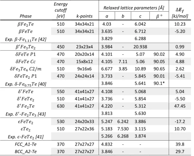
6. Results and discussion of DFT calculations
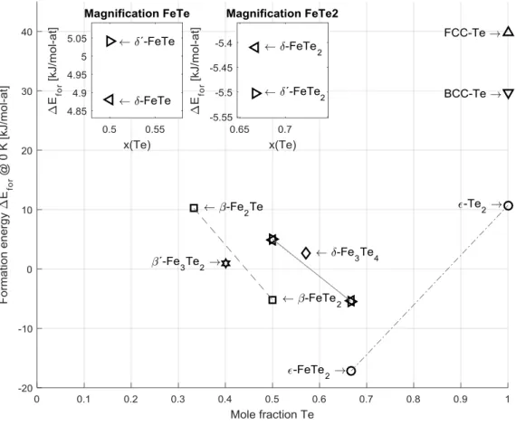
The lattice stability of FCC_A1 and BCC_A2 tellurium were evaluated and used in the modeling of Te solubility in the iron terminal phases. The formation energies of the end-members (Table 3) of the , , , and phases are summarized in Table 4 together with converged parameters. Figure 1 displays the formation energies evaluated in this work, with magnification on the region. In phases of the NiAs-type structure, here and , some atoms may be interstitially dissolved in the trigonal-bipyramidal holes [31]. In order to test the possibility of Fe atoms occupying those sites, the formation energy of the end-member - , i.e. (Fe)1(Fe)1(Fe)2(Te)2, with purely hypothetical
interstitial iron in the trigonal-bipyramidal sites was evaluated; the highly positive result (Table 4) indicated that it is not a stable configuration, and iron was not added to the third sublattice for the modeling.
As expected, the formation energies of and show that the former, monoclinic configuration is slightly more stable at lower Te content while the latter, hexagonal one is stable at higher Te content (Figure 1); as seen in Table 4, their energies are very close. The triclinic was calculated with lattice parameters equivalent to the monoclinic , hence the very small difference in energy. The unit cell with space group has the composition of 57.14 at% Te, lying within the stability region of the phase, although the calculation was still made at 0 K. After the lattice parameters were optimized by static calculations, the volume was relaxed followed by a shape relaxation. The angle drastically changed from about 90.5 to 85 , because the Fe(1) interstitials were offset from the preferred octahedral coordination with surrounding Te atoms, making it dynamically unstable. Subsequently, all degrees of freedom were relaxed, and the Fe(1) atoms moved into the octahedral sites. The cell volume decreased by 5 %, shifted back to and the formation energy drastically decreased from 12 kJ/mol to 2.62 kJ/mol (Table 4). It also obtained a net zero magnetic moment, in contrast with the other magnetic and phase end-members. While has a lower formation energy than and , they are evaluated at different composition and therefore not directly comparable. The phase was relaxed in the crystal structure of the ternary of the
rhombohedral space group 160. The calculated enthalpy of formation is positive as the end-member composition lies outside of the region of stability. However, it is small and the phase is stable only at high temperatures; therefore it should not be ruled out that this is the structure of the phase.
Table 4: Relaxed lattice parameters and 0 K formation energies ( ) from DFT calculations on Fe-Te end-members. is only written out if it is not 90 . *: in triclinic setting equivalent to in monoclinic setting.
Energy cutoff
[eV] k-points
Relaxed lattice parameters [Å] [kJ/mol] Phase a b c 510 34x34x21 4.03 - 6.042 10.23 510 34x34x21 3.635 - 6.712 -5.20 Exp. - [42] 3.829 6.288 450 23x23x4 3.984 - 20.938 0.99 470 20x20x14 4.101 - 5.07 90.02 4.90 470 15x8x12 4.105 7.11 5.06 90.05 4.88 510 9x16x6 6.677 3.85 10.89 90.65 2.62 470 24x24x14 3.733 - 5.845 90.01 -5.41 Exp. - [40] 3.846 5.641 90.1* 550 41x41x27 4.108 - 5.068 5.04 510 41x41x27 3.736 - 5.854 -5.50 630 41x41x27 4.220 - 5.312 47.45 Exp. - [43] 3.813 5.630 530 24x20x33 5.247 6.242 3.886 -17.2 510 27x22x36 5.183 7.530 3.115 10.70 Exp. - [41] 5.266 6.268 3.874 FCC_A1-Te 370 27x27x27 4.832 - - 39.8 BCC_A2-Te 370 27x27x27 3.846 - - 29.7
Figure 1: Enthalpy of formation at 0 K relative to BCC_A1 and A8 reference states for Fe and Te, respectively, evaluated via DFT. Diagram inserts separate the and phases. Lines guide the eyes between end-members of the same phase.
7. Results and discussion of thermodynamic assessment
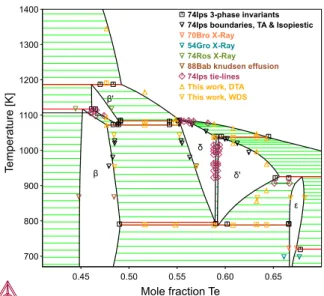
Figure 2 shows the final calculated phase diagram compared with the liquidus data by Ipser et al. [30] and Chiba [38]. Figure 3 is magnified in the region of interest of the intermediate phases, compared with selected experimental data. The different phase regions compared with experimental phase diagram data is discussed in the subsections below, followed by a comparison of thermodynamic data, and finally a comparison of Gibbs energy of formation of iron tellurides with previous predictions.
7.1. Liquid and terminal phases
The liquidus of the Fe-Te system (see Figure 2) is entirely consistent with the data of Ipser et al. [30], and that of Chiba [38], excluding the two points that deviate most from the main body of data. As observed in Figure 3, the description also agrees well with the data gather via DTA in Part I:
Experimental study, most importantly the iron-rich high-temperature point, consistent with the
previously proposed steep liquidus [30], thus supporting the liquid miscibility gap. Although not shown in these figures, no inverted miscibility gap is found up to 6000 K.
The solubility of the - phase fits the tie-lines by Ipser et al. and those gathered in Part I. The subregular solution parameter optimized to achieve this also resulted in a gamma loop (Figure 2), as Okamoto et al. [44] predicted in their review.
7.2. and phases
In order to fit the boundaries measured in this work, consistent with the tie-lines by Ipser et al. [30], in addition to the boundary data, the phase would require an unnatural shape. The rather strong peak found via DTA of sample FT47_D (Part I, Fig. 4) indicates that the invariant extends up to this point, while maintaining consistency with the tie-lines. The present model seems to give a more natural shape of the phase, than it would have by following all published tie-lines. The phase boundary compositions from isothermal heat treatments in this work are not accurate enough to conclude on data inconsistency.
7.3. / and phases
The phase fit within error margins to the selected data, but including the phase made it difficult, and compromises were necessary to avoid introducing an unrealistic number of interaction terms. One would either have to elevate the peritectic temperature of phase formation, incline the miscibility gap, or lower the eutectoid invariant arrests of the phase. All those compromises were assessed, and it was eventually selected to fit the invariant reactions at the expense of the / and ’/ boundaries, since the invariant reactions were more accurately determined via DTA. Since no phase composition was found in the isothermal heat treatments, the tie-lines that were intended to be in equilibrium with the phase are treated as tie-lines. The phase boundaries fits the experimental data much better when the phase is suspended, as shown in the phase diagram of Figure 4.
7.4. phase
The phase description did not fit well with the evaluated enthalpy of formation together with the peritectic invariant temperature; when the parameters instead were fitted to the phase diagram, the enthalpy of formation coincided very well with the calorimetric measurements by Vladimirova et al. [9] and the - end-member formation energy evaluated via DFT in this work, as seen in Figure 6. The model is in addition consistent with the and tie-lines evaluated from samples FT77_T1 and FT65_T2.
7.5. Thermodynamic activity, chemical potential and heat capacity
Figure 5 presents the calculated tellurium activity with varying composition at 700 C, relative to the liquid phase, compared with isopiestic [6] and partial pressure data [2,4,5]. Figure 7 and Figure 8 similarly present the calculated chemical potential of iron relative to BCC at 750 and 835 K,
respectively, compared with the EMF data by Geiderikh [1]. It proved difficult to fit all activity data sets together. Therefore, all models were optimized to fit the isopiestic activity data by Ipser et al. (Figure 5), since they vary in both temperature and composition, and then compare with the EMF and partial pressure data sets. As can be seen in the figures, the thermodynamic description agrees very well with the isopiestic activity data, and sufficiently well with partial pressure and EMF data. Figure 9 and Figure 10 show the calculated heat capacity of the and phases, respectively, and they agree well with selected experimental data. The magnetic transition in the phase at 67 K was not modeled, and the single point seen in Figure 9 that strongly deviates from the linear behavior was regarded as an artifact and ignored. The heat capacity of the phase (Fig. Figure 10) was only fitted to the work by Westrum et al. [10]. Mikler et al. [11], in their heat capacity measurement on an sample, noted an anomalous increase in at higher temperature that could be due to precipitation of pure tellurium. Figure 11 shows their measured composition and temperature range relative to the phase diagram; it seems probable that their sample initially contained small amounts of pure tellurium. Figure 12 shows the calculated heat capacity for that composition compared with their data, and indeed it seems possible that a contribution from the tellurium gives rise to an increase in of such a magnitude.
7.6. Application: Predicted formation energy of iron tellurides
The final Gibbs energy models of the Fe-Te system are listed in Table 1 in the Appendix. The terms in the - and the - end-members are notably high. This is because these phases are very stable, as shown by the magnitude of the enthalpy of formation in Figure 6, thus making it necessary to have such large positive values in order to destabilize them at higher temperatures. Table 5 shows calculated Gibbs energy of formation compared with estimated values available in literature, with reasonable agreement. The properties at the Te rich side of the phase show larger disagreement than the Fe rich side, due to the slightly higher enthalpy of formation from this description. The enthalpy of formation of the phase has a large disagreement from derived data, but the description agrees better with formation enthalpy from DFT and calorimetric data on samples (see Figure 6) [9].
Table 5: Enthalpies and Gibbs energies of formation of iron tellurides compared with data from literature.
Formula Phase Temp. [K]
[kJ/mol-f.u.]
(Ref. value)
[kJ/mol-f.u.]
(Ref. value) Ref.
298.15 -21.2 (-21.1) -17.6 (-17.2) [45] 298.15 -24.0 (-29.7) -20.2 (-27.8) [45] 298.15 -19.5 (-23.46) [8] 800 -15.6 (-15.86) [4] 4 298.15 -51.1 (-58.3) -51.9 (-65.8) [39]
4 Here calculated as since
Figure 2: Calculated Fe-Te phase diagram compared with published liquidus data.
Figure 3: Calculated Fe-Te phase diagram magnified in the region of interest of intermediate phases, compared with selected experimental phase diagram data.
Figure 4: Calculated phase diagram of the same description as Fig. 2, with the phase suspended. Note the closer fit of the left solvus of to experiment.
Figure 5: Calculated tellurium activity at 700 C relative to the liquid phase, of the Fe-Te system compared with experimental data.
Figure 6: Calculated molar enthalpy of formation of the Fe-Te system at room temperature, compared with published data and DFT data of this work.
Figure 7: Calculated iron potential, relative to the BCC phase, of the Fe-Te system at 750 K compared with the EMF measurements of Geiderikh et al. [1].
Figure 7: Calculated iron potential, relative to the BCC phase, of the Fe-Te system at 835 K compared with the EMF measurements of Geiderikh et al. [1].
Figure 8: Calculated heat capacity of the phase compared with experimental data.
Figure 9: Calculated heat capacity of the ϵ phase compared with experimental data.
Figure 10: The composition and temperature range of the CP measurement of Mikler et al. [11].
Figure 11: CP calculated for the composition in Fig 11, i.e.
0.676 at% Te, compared with the experimental data of Mikler et al. [11].
8. Conclusions and future work
In this work a thermodynamic model of the Fe-Te system was developed. The description accurately predicts thermodynamic and phase diagram data available in literature. The and phases were described with a single three-sublattice model separated by a miscibility gap, since they belong to the same structure family, and should experience full solubility in the ternary Fe-Ni-Te system. The design of sublattice models within the Compound Energy Formalism enabled the use of end-member energies of formation estimated via DFT calculations in the optimization. The model may be used both with and without the phase: if it is excluded from the phase diagram, the phase boundary fits experimental data better without negatively affecting other properties. The use of an ionic liquid model with an ordered FeTe associate accommodates for a liquid miscibility gap.
It is recommended to perform a more detailed DFT analysis on the phase in order to conclude on its space group symmetry. Supercells with random and ordered partial occupation of Fe sites can make the and formation energies more comparable. Finite temperature calculations would enhance the accuracy, as well as indicate if the phase is stabilized by entropy.
The different possible ordered magnetic structures of the phase are of interest for the semi- and superconductor industries, and the thermodynamic model can be modified to accommodate for this. The proposed model is deemed accurate enough for the purpose of modeling internal fuel pin corrosion in nuclear reactors.
Acknowledgements
The authors would like to thank the Swedish Research Council (Vetenskapsrådet) for the funding of the project. C.-M. wishes to thank his colleagues at KTH and CEA for the advice in thermodynamic modeling: Drs Bonnie Lindahl and Nathalie Dupin for advice on the modeling, and Prof. Andrei Ruban for lending his advice on the DFT calculations.
C.-M. wishes to thank Prof. Herbert Ipser for the discussions they have had regarding the modelling of the phases of the Fe-Te system, and especially for personally lending him a copy of his thesis on the system.
Last but not least, C.-M. extends thanks to the components of Nomad Chemistry for advice and support during his work.
Bibliography
[1] V. A. Geiderikh, Y. I. Gerasimov och A. V. Nikol'skaya, ”Thermodynamic Properties of Iron-Tellurium Alloys in the Solid State,” (TR) Proceedings of the Academy of Sciences of the USSR.
Physical Chemistry section., vol. 137, pp. 394-351, 1961.
[2] B. Saha, R. Viswanathan, M. Sai Baba, D. Darwin Albert Raj, R. Balasubramanian, D. Karunasagar och C. K. Mathews, ”High-temperature mass-spectrometric studies of Te(s) and FeTe0.9(s),”
Journal of Nuclear Naterials, vol. 130, pp. 316-325, 1985.
[3] M. Sai Baba, R. Viswanathan, R. Balasubramanian, D. Darwin Albert Raj, B. Saha och C. K. Mathews, ”Vaporization thermodynamics of (iron+tellurium): a high-temperature mass-spectrometric study,” Journal of Chemical Thermodynamics, pp. 1157-1173, 1988.
[4] R. Prasad, S. Mohapatra, V. S. Iyer, Z. Singh, V. Venugopal och D. D. Sood, ”Thermodynamics of iron telluride (Fe0.540Te0.460),” Journal of Chemical Thermodynamics, vol. 20, pp. 453-456, 1988.
[5] V. Piacente och P. Scardala, ”Study of the vaporization behaviour of iron monotelluride,” Journal
of Alloys and Compounds, vol. 184, pp. 285-295, 1992.
[6] H. Ipser och K. L. Komarek, ”Thermodynamic Properties of Iron-Tellurium Alloys,” Monatshefte
für Chemie, vol. 105, pp. 1344-1361, 1974.
[7] C. Fabre, ”heats of Formation of Some Telluride Crystals,” Comptes Rendus Chimie, vol. 105, pp. 277-280, 1887.
[8] N. K. Shukla, R. Prasad, K. N. Roy och D. D. Sood, ”Standard molar enthalpies of formation at the temperature 298.15 K of iron telluride (FeTe0.9) and of nickel telluride (Ni0.595Te0.405),”
Journal of Chemical Thermodynamics, vol. 22, pp. 899-903, 1990.
[9] V. A. Vladimirova, R. A. Zvinchuk, M. P. Morozova och O. Y. Pakrativa, ”Enthalpy of Formation and Structure of Non-stoichiometric Iron Telluride,” Tr: Russian Journal of Physical Chemistry, vol. 53, nr 3, pp. 346-348, 1982.
[10] E. F. Westrum, C. Chou och F. Grønvold, ”Heat Capacities and Thermodynamic Properties of the Iron Tellurides Fe1.11Te and FeTe2 from 5 to 350 K,” The Journal of Chemical Physics, vol. 30, nr 3, pp. 761-764, 1959.
[11] J. Mikler, H. Ipser och K. L. Komarek, ”Spezifische Wärmen von FeTe und FeTe2 von Raumtemperatur bis 900 K,” Monatshefte für Chemie, vol. 105, pp. 977-986, 1974.
[12] A. Mani, J. Janaki, T. Geetha Kumary, N. Thirumurugan, S. Kalavathi och A. Bharathi, ”Specific heat studies on pristine and oxygenated iron tellurides,” Solid State Communications, vol. 151, pp. 1210-1213, 2011.
[13] T. Maekawa och T. Yokokawa, ”Enthalpies of infinitely dilute solutions of transition metals in liquid tellurium,” Journal of Chemical Thermodynamics, vol. 7, pp. 505-506, 1975.
[14] D. D. Wagman, W. H. Evans, V. B. Parker, R. H. Schumm, I. Halow, S. M. Bailey, K. L. Churney och R. L. Nuttal, ”The NBS tables of chemical thermodynamic properties,” Journal of Physical and
Chemical Reference Data, vol. 11, 1982.
[15] Y. V. Rumyantsev, G. M. Zhiteneva och F. M. Bolondz, ”Thermal Stability of Selenides and Tellurides of Iron and Nickel,” Tr. Vost. Sibirisk Filialia, Akad. Nauk SSSR, vol. 42, p. 114, 1962. [16] P. E. Blochl, ”Projector augmented-wave method,” Physical Review B, vol. 50, p. 17953, 1994. [17] G. Kresse och D. Joubert, ”From ultrasoft pseudopotentials to the projector augmented-wave
method,” Physical Review B, vol. 59, p. 1758, 1999.
[18] G. Kresse och J. Hafner, ”Ab initio molecular dynamics for liquid metals,” Physical Review B, vol. 47, p. 558, 1993.
[19] G. Kresse och J. Hafner, ”Ab initio molecular-dynamics simulation of the
liquid-metal-amorphous-semiconductor transition in germanium,” Physical Review B, vol. 49, p. 14251, 1994. [20] G. Kresse och J. Furthmüller, ”Efficiency of ab-initio total energy calculations for metals and
semiconductors using a plane-wave basis set,” Computational Materials Science, vol. 6, p. 15, 1996.
[21] G. Kresse och J. Furthmüller, ”Efficient iterative schemes for ab initio total-energy calculations using a plane-wave basis set,” Physical Review B, vol. 54, p. 11169, 1996.
[22] J. P. Perdew, K. Burke och M. Ernzerhof, ”Generalized gradient approximation made simple,”
Physical Review Letters, vol. 77, p. 3865, 1996.
[23] J. P. perdew, K. Burke och M. Ernzerhof, ”Erratum: Generalized gradient approximation made simple,” Physical Review Letters, vol. 78, p. 1396, 1997.
[24] P. Beiss, ”Iron and steel: Manufacturing route,” i Landolt-Börnstein - Group VIII Advanced
Materials and Technologies 2A1, P. Beiss, H. Ruthardt och H. Warlimont, Red., Berlin,
Springer-Verlag, 2003, pp. 5.1-5.20.
[25] SpringerMaterials, ”Tellurium (Te) elastic moduli,” i Landolt-Börnstein - Group III Condensed
Matter 41C, U. R. M. S. O. Madelung, Red., Berlin, Springer-Verlag, 1998, p. Online Document
1279.
[26] M. Hillert, ”The compound energy formalism,” Journal of Alloys and Compounds, vol. 320, pp. 161-176, 2001.
[27] H. L. Lukas, S. G. Fries och B. Sundman, Computational Thermodynamics. The Calphad Method., New York: Cambridge University Press, 2007.
[28] E. E. Rodriguez, C. Stock, P. Zajdel, K. L. Krycka, C. F. Majkrzak, P. Zavalij och M. A. Green, ”Magnetic-crystallographic phase diagram of the superconducting parent compound Fe1+xTe,”
Physical Review B, vol. 84, p. 064403, 2011.
[29] G. Åkesson och E. Røst, ”The Crystal Structure of Fe.28Ni.28Te.44,” Acta Chemica Scandinavica, vol. 27, pp. 79-84, 1973.
iron-Tellurium Phase Diagram,” Monatshefte für Chemie, vol. 105, pp. 1322-1334, 1974. [31] I. Jandl, H. Ipser och K. W. Richter, ”Thermodynamic modelling of the general NiAs-type
structure: A study of first principle energies of formation for binary Ni-containing B8
compounds,” CALPHAD: Computer Coupling of Phase Diagrams and Thermochemistry, vol. 50, pp. 174-181, 2015.
[32] M. Hillert, B. Jansson, B. Sundman och J. Ågren, ”A two-sublattice model for molten solutions with different tendency for ionization,” Metallurgical Transactions A, vol. 16, nr 1, pp. 261-266, 1985.
[33] A. V. Davydov, M. H. Rand och B. B. Argent, ”Review of Heat Capacity Data for Tellurium,”
Calphad, vol. 19, nr 3, pp. 375-387, 1995.
[34] B. Cheynet, P.-Y. Chevalier och E. Fischer, ”Thermosuite,” Calphad, vol. 26, nr 2, pp. 167-174, 2002.
[35] G. V. Belov, V. S. Iorish och V. S. Yungman, ”IVTANTHERMO for Windows - Database on Thermodynamic Properties and Related Software,” Calphad, vol. 23, nr 2, pp. 173-180, 1999. [36] A. T. Dinsdale, ”SGTE data for pure elements,” CALPHAD, vol. 15, nr 4, pp. 317-425, 1991. [37] J. O. Andersson, T. Helander, L. Höglund, P. F. Shi och B. Sundman, ”Thermo-Calc and DICTRA,
Computational tools for materials science,” Calphad, vol. 26, pp. 273-312, 2002.
[38] S. Chiba, ”The Magnetic Properties and Phase Diagram of Iron Tellurium System,” Journal of the
Physical Society of Japan, vol. 10, nr 10, pp. 837-842, 1955.
[39] M. Sai Baba, R. Viswanathan och C. K. Mathews, ”Thermodynamic and Phase Diagram Studies on Metal-Tellurium Systems Employing Knudsen Effusion Mass Spectrometry,” Rapid
communications in mass spectrometry, vol. 10, pp. 691-698, 1996.
[40] F. Grønvold, H. Haraldsen och J. Vihovde, ”Phase and Structural Relations in the System Iron Tellurium,” Acta Chemica Scandinavica, vol. 8, pp. 1927-1942, 1954.
[41] G. Brostigen och A. Kjekshus, ”Compounds with the Marcasite Type Crystal Structure V. The crystal structure of FeS2, FeTe2 and CoTe2,” Acta Chemica Scandinavica, vol. 24, nr 6, pp. 1925-1940, 1970.
[42] J. Leciejewicz, ”A Neutron Diffraction Study of Magnetic Ordering in Iron Telluride,” Acta
Chemica Scandinavica, vol. 17, pp. 2593-2599, 1963.
[43] J. B. Ward och V. H. McCann, ”On the 57Fe Mössbauer spectra of FeTe and Fe2Te3,” Journal of
Physics C: Solid State Physics, vol. 12, pp. 873-879, 1979.
[44] H. Okamoto och L. E. Tanner, ”The Fe-Te (Iron-Tellurium) System,” Bulletin of Alloy Phase
Diagrams, vol. 11, nr 4, pp. 371-376, 1990.
[45] C. K. Mathews, ”Thermochemistry of transition metal tellurides of interest in nuclear technology,” Journal of Nuclear Materials, vol. 201, pp. 99-107, 1993.
[46] G. S. Mann och L. H. Van Vlack, ”Fe1.2Te-MnTe Phase Relationships in the Presence of Excess Iron,” Metallurgical Transactions B, vol. 8B, pp. 53-57, 1977.
[47] H. Kopp, ”Investigations of the Specific Heat of Solid Bodies,” Philisophical Transactions of the
Royal Society of London, vol. 155, pp. 71-202, 1865.
[48] C. Adenis, V. Langer och O. Lindqvist, ”Reinvestigation of the Structure of Tellurium,” Acta
Appendix
Table 1: Sublattice models, with corresponding Wyckoff positions, used in the assessment of the Fe-Te system are presented with the resulting converged thermodynamic parameters. GLIQFE, GLIQTE, GHSERFE and GHSERTE are pure element thermodynamic functions from the SGTE PURE5 database [33-36].
Liquid: (Fe+2)P(Va-Q,FeTe0,Te0)Q
: (Fe,Va)3(Te)2 Wyckoff: (3a)3(3a)2
: (Fe)1(Te)1(Fe,Va)1 Wyckoff: (2a)(2c)(2c)
and : (Fe,Va)1(Fe,Va)1(Te)2 Wyckoff: (1a)(1b)(2d)
: (Fe,Va)1(Te)2 Wyckoff: (2a)(4g)
: (Fe)1(Te)1.183
BCC_A2: (Fe,Te)1(Va)3 Wyckoff: (2a)(6b) FCC_A1: (Fe,Te)1(Va)1 Wyckoff: (4a)(4b)
Table 2: Table of invariant equilibria calculated from the thermodynamic model in the present work, compared with the phase diagram review by Okamoto and Tanner [44].
Reaction at.% Te T [ ] Ref. T [ ] [44] Reaction type
0 1537.8 1538 Melting 0 1394.3 1394 Allotropic 0 911.7 912 Allotropic 7.70 1447.1 ~1500 [46] Monotectic 46.10 913.5 914 Peritectic 45.17 843.9 844 Peritectoid 55.30 810.6 812 Peritectic 54.19 807.3 809 Peritectoid 48.86 799.1 800 Eutectoid 54.19 636.3 636 Eutectoid 58.94 522.9 565±15 [30] Eutectoid 59.30 515.3 519 Eutectoid 59.28 764.0 766 Peritectic 67.98 652.5 649 Peritectic 98.96 446.9 448 Eutectic 100 449.5 449.57 Melting


![Table 3: Sublattice models used for solution phases of the Fe-Te system. The gas phase is taken from the SGTE SSUB5 [33-35]](https://thumb-eu.123doks.com/thumbv2/123doknet/13327016.400470/8.892.103.780.348.660/table-sublattice-models-solution-phases-phase-taken-sgte.webp)