Efficient and robust reconstruction of botanical branching structure from laser scanned points

HAL Id: inria-00436480

https://hal.inria.fr/inria-00436480

Submitted on 26 Nov 2009

HAL is a multi-disciplinary open access

archive for the deposit and dissemination of

sci-entific research documents, whether they are

pub-lished or not. The documents may come from

teaching and research institutions in France or

L’archive ouverte pluridisciplinaire HAL, est

destinée au dépôt et à la diffusion de documents

scientifiques de niveau recherche, publiés ou non,

émanant des établissements d’enseignement et de

recherche français ou étrangers, des laboratoires

Efficient and robust reconstruction of botanical

branching structure from laser scanned points

Dong-Ming Yan, Julien Wintz, Bernard Mourrain, Wenping Wang, Frédéric

Boudon, Christophe Godin

To cite this version:

Dong-Ming Yan, Julien Wintz, Bernard Mourrain, Wenping Wang, Frédéric Boudon, et al.. Efficient

and robust reconstruction of botanical branching structure from laser scanned points. CAD/Graphics

2009, Aug 2009, Yellow Mountain City, China. pp.572-575. �inria-00436480�

Efficient and robust tree model reconstruction

from laser scanned data points

Dong-Ming Yan, Julien Wintz, Bernard Mourrain, Wenping Wang,

Frédéric Boudon and Christophe Godin

December 4, 2008

Abstract

This paper presents a reconstruction pipeline for recovering a tree model from laser scanned data points. The process is made up of three main steps: segmen-tation, reconstruction and modeling. Based on a variational k-means clustering algorithm, cylindrical components and ramified regions of data points are identi-fied and located. An adjacency graph is then built from neighborhood information of components. Simple heuristics allow us to extract a tree structure and identified branches from the graph. Finally, a B-spline model is computed to give a compact and accurate reconstruction of the branching system.

I.3.3Computer GraphicsMethodology and Techniques

1

Introduction

Due to the complexity and the diversity of plant shapes, the construction of plant ge-ometric models is still a challenging problem for both computer graphics and biology. Two major approaches have been developed so far.

On the one hand, plant models can be simulated by procedural methods. With various degrees of realism these methods can mimic the development of plant axes to create complex branching structures as an emerging property of prescribed develop-mental rules. Global constraints can be added to these local-to-global procedures to control the overall shape of the resulting models [WP95,PHHM97,SRDT01,BPF∗_03].

These methods have proved very successful to build up various types of plant models ranging from herbs to trees. However, these procedural methods have two important limits. First, modelers must have some expertise about the growth of the plant they want to model in order to design the developmental rules or tune the parameters. Sec-ond, if one wants to build up a model corresponding to the exact 3D structure of a plant, these methods do not give any hint on how to organize measurements on the observed plant to build up an accurate computer representation.

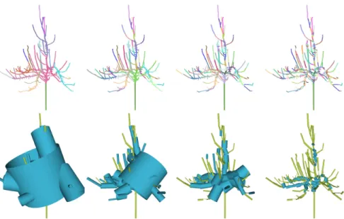
Figure 1: Tree model reconstruction. From left to right: 1) Scanned data of an apple tree; 2) Segmentation result, different colors for different clusters; 3) Branch identifica-tion result. The color of each branch is the same as its starting cluster; 4) Final B-spline surface representation of tree branches.

1.1

Data acquisition

To address the latter issue, researchers in both biology and computer graphics have designed methods to directly capture the 3D plant structures in computers using dif-ferent types of sensors and adapted measurement protocols. Contact methods were initially developed by agronomists and plant modelers to digitize moderate size plants. Magnetic [SRG97] or sonic [?, ?] devices were used to allow the observer to get the position and orientation of each plant organ using a 3D pointer. These methods make it possible to create 3D branching models faithful to the observed plant topology and geometry [GCS99]. However, they are extremely time-consuming (the digitizing of a single tree contained in a 3m3 bounding box takes 1 day for 2 persons on average). To alleviate this difficulty, researchers have considered the use of other types of sensors. The possibility to reconstruct plant structures using digital cameras was tested in dif-ferent works [SRDT01, RMD04, PS05]. One or several photographs are taken around the plant from different viewing angles which make it possible to extract geometric and optical characteristics of the plant structure using image analysis techniques. In general, the global 3D silhouette of the plant is first extracted. Then, depending on the application, additional traits are extracted from the images: local opacity and texture of elementary cell volumes [RMD04], foliage characteristics such as crown volume or total leaf area of the plant [PS05] or even approximations of the plant branching sys-tem using a procedural method to grow a plant within the bounding volume [SRDT01]. These approaches are easy to apply to medium-size isolated plants, and give good re-sults for inferring global characteristic of plant foliage. However, identifying individ-ual organs from 2D photographs (trunk, branches or individindivid-ual leaves) is still a limiting issue [TCH07].

More recently, to capture accurately the geometry of individual plants, researchers developed techniques based on 3D laser scanners. The additional depth information associated with each pixel of the scanned image makes it possible to recover the po-sition of the plant structure in 3D and some of its optical properties. This informa-tion has been recently exploited at the organ level to reconstruct leaf surfaces with

accuracy and provide parameters that can be further exploited in light interception models, [CAD∗_{ar]. At plant level, first tests for the reconstruction of simple}

branch-ing systems were carried out by [PGW04]. A more complete method was proposed by [XGC07] who introduced a method for reconstructing complete plant models from 3D scans. This method makes it possible to infer the topology and the geometry of the plant structure with accuracy. However, if the main branching system (trunk and low order branches) is usually accurately reconstructed, the rest of the branching system (finer branch of high order) is inferred via an additional stochastic procedural method. The result was assessed via visual inspection.

1.2

The reconstruction problem

In this paper, we consider the problem of reconstructing complete branching systems faithful to observed tree from 3D laser scans. Since branches may be hidden by leaves, we restrict our approach to trees without leaves (e.g. temperate species observed in winter for example). Our goal is to obtain a compact model that reflects with accuracy the observed branching system. In particular, from the clouds of points obtained from the 3D laser scans, the method should be able to:

• identify the different plant axes. Ambiguity in axis recognition may come from two main phenomena i) different axes may have parts that are close to each other in the 3D space, ii) parts of the axes may be hidden by other axes.

• identify axis connections. Connections between axes may also be hidden or partially sampled, making it difficult to guess the correct hierarchy of axes. • estimate axis geometry. One key issue of the reconstruction is to recover the axis

diameter variation from the partial sampling of the axis surface (each scanned imaged only contains a part of this surface).

We propose hereafter a chain of algorithms that is aimed to meet these require-ments. First, the main trunk and branch structures of the tree are identified during the reconstruction process. Each branch is represented by a sweeping surface along its skeleton, with various radius determined from scanned data. We choose this parametric representation since it is compact, efficient to manipulate and easy to edit. The overall reconstruction process is illustrated on an apple tree in Fig. 1.

The main contributions of this paper include:

• A complete framework for tree structure reconstruction from scanned point cloud. The reconstructed model is represented by a set of sweeping surfaces along the skeleton of the tree;

• A new variational point cloud segmentation framework is proposed (Section 2), which locates the cylindrical and branching regions efficiently;

• Simple heuristics are proposed to reconstruct branching structure of trees from segmentation result (Section 3);

1.3

Related work

Recently, with the increasing requirements for the realism of the visual effect, re-searchers begin to integrate computer vision techniques with computer graphics for tree modeling and rendering. A lot of works have been done on image based [RMD04, QTZ∗_{07, NFD07, TZW}∗_{07, TCH07] and sketch based plant modeling [OOI05, IOI06a,}

IOI06b]. The input data could be a sequence of photographs, two images of different views or some simple 2D sketches, and the output is a 3D tree model, which has sim-ilar visual effect with the input images. Image based modeling techniques are usually used for realistic rendering purpose. Since the output model is synthesized instead of reconstructed from real data, which is different from the real geometry of a tree. It cannot be used for agronomy or biology analysis and simulation.

Relatively little work has been done on tree reconstruction from scanned point data in literature. Pyysalo et al. [PH02] propose a method to reconstruct tree crowns from scanned data for feature extraction. But their purpose is to compute statistic infor-mation of forest, which is far from the real branch structure of a tree. Gorte and Pfeifer [GP04] use a 3D morphology method to segment and extract the skeleton from point data. As reported by the authors, the space and time become the bottleneck of their method, which increases with the third power of the resolution. It becomes im-possible for large point sets with millions of points. Based on the segmentation method of [GP04], Pfeifer et al. [PGW04] present a method to reconstruct tree models by fit-ting cylinders for segmented data. Because the incompleteness of the scanned data, the fitted cylinder can be far from the real branch. Instead of fitting, we use bounding cylinder to approximate the radius of the branches, which is more efficient and more robust than cylinder fitting.

The most related work to our approach is [XGC07]. In this work, the input scanned data are first connected together to form a graph. The main skeleton of the tree is pro-duced by clustering points with same quantized distance to the root and the clusters are used to generate skeleton of tree. The other small branches and leaves are synthesized then. But the topology of the skeleton of their method may not be a tree structure, which often contain loops, as we will discuss later, and the resulting skeleton is not geometric faithful since only the distance to the root is used for segmentation.

In our work, a novel skeletonisation method based on variational geometric clus-tering is proposed. Further more, the main trunk and branches are identified and we produce a more compact and topological correct representation of branch structure of the tree. We refer the reader to [BMG06] for a survey on computer representation and efficient rendering techniques of trees.

1.4

Outline

Our approach is composed of three main steps: segmentation, branch reconstruction and modeling. Section 2 introduces a new variational approach for point cloud data segmentation. Section 3 presents an efficient algorithm for reconstructing branches from the clusters obtained in the segmentation phase. Finally, a flexible interactive modeling system is introduced in Section 4. Experimental results are given in Section 5 before we draw our conclusions in Section 6.

2

Segmentation

Laser scanned real trees produce a huge amount of unstructured data, which naturally feature many cylindrical shapes – the branches – see Fig. 1 (left) for example. The aim of the segmentation step is to partition the data into connected sub clusters, each cluster being bounded by a circular cylinder as tightly as possible. We will first give the problem definition and then explain our variational point cloud segmentation algorithm in detail.

Let P = {pi, i= 1, . . . , N} be a dense point set of a tree model. A segmentation

C of P is a set of clusters {Ci, i= 1, . . . , n}, such thatSni=1Ci= P, where (n ≪ N),

and Ci∩ Cj= ∅, for any i 6= j. Each cluster Ci contains a sub set of the point set, i.e.

Ci= {pik, k= 1, . . . , ni}, where ni= |Ci|. We propose a hybrid approach to segmenting

the point set and detecting cylinder components at the same time. The following are the main steps of our segmentation algorithm:

1. Preprocessing: A kd-tree representation of the point set P is constructed to facilitate the retrieval of neighboring points of any data point in the point set P.

2. K-means clustering: The preprocessed point set is segmented into clusters us-ing the Lloyd iteration [Llo82], which minimizes the energy function defined in Eqn. 1 below. Each cluster is a connected sub-graph of the kd-tree.

3. Cylinder detection: For each cluster Ciobtained from the k-means clustering,

a minimal bounding cylinder is computed to measure the tightness of the bounding volume. If the bounding volume satisfies some criteria, the cluster Ciis flagged as fixed

and will not change anymore.

4. Subdivision: If there remain clusters that cannot be bounded by a cylinder tightly or the number of points in these clusters is more than a user specified value, then they are subdivided and the process goes back to step 2. Otherwise, the algorithm terminates.

2.1

Preprocessing

Since a point set features no adjacency relationship, the neighborhood of a point pi

is represented by its k-nearest neighbor points, Nk(pi). A kd-tree data structure is

constructed for efficient neighborhood search. We use ANN library [MA06] for kd-tree construction in our implementation and choose k = 8 in all our experiments.

2.2

K-means clustering

In this step, we want to segment the input point cloud P into a set of clusters C, re-flecting the main structure of the tree, where all points belonging to a cluster form a connected component.

To this end, we propose a variant of the well known k-means clustering technique, which efficiently segments the point set while keeping the connectivity of neighbor-hood at the same time. The clustering algorithm is adapted from the distortion mini-mization flooding algorithm used for mesh segmentation [CSAD04]. The Lloyd itera-tion [Llo82] is used to repeat between clustering and centroid replacement. The energy

Figure 2: Intermediate results of the hybrid segmentation algorithm. Top row: segmen-tation result. From left to right, the number of clusters is 19, 60, 96, 214, respectively. Bottom row: bounding cylinders of corresponding clusters. The green cylinders are fixed and those blue ones are unfixed.

function of a segmentation is defined such as in k-means clustering:

E(P, C) = n

∑

∑

∑

where ciis the center of the cluster Ciand d(pj,ci) is the Euclidean distance between

the point pj and the center ci. The following is the detailed description of our

varia-tional segmentation algorithm.

1. Initialization: To start the algorithm, we randomly select n points {si,i= 1...n}

as initial seeds to define n clusters {Ci,i= 1...n}, where n is a user input parameter.

2. Clustering: Once a seed point is found for each cluster, we segment the point set by growing a region for each cluster according to these seeds. Each point pi is

equipped with a flag to indicate whether this point is selected or not. The flag of each seed point is set to selected and the flags of all other points are set as unselected at beginning. The implementation of the clustering algorithm is similar to that proposed in [CSAD04]. We use kd-tree instead of the connectivity information of triangle mesh. The reader is referred to [CSAD04] for details.

3. Updating: Once the clusters Cihave been identified, a new seed point sineeds

to be selected from Ciin order to compute the next generation of clusters. This is done

as follows. First the center ciof each cluster Ciis computed. We choose

si= arg min pj∈Ci

, as the new seed point; that is, we use the data point pjin Cithat is closest to cias the

new seed. Next the total error Eiter(P, C) of the energy function is evaluated, where

iter is the number of iterations done so far. Should a maximal number of iteration be reached or should the error between two iterations be smaller than a user defined threshold (i.e. |Eiter− Eiter−1| < ε), the iteration stops; otherwise we go to step 2.

2.3

Cylinder detection

The k-means clustering terminates when it has produced a well shaped partition of the input point cloud. Since the shape of branches is naturally cylindrical (at least locally), we consider extracting cylinder components from the partition.

In order to compute bounding cylinders, the principle direction of each cluster Ci

is computed. The eigenvector of the covariance matrix of Ciwith largest eigenvalue is

selected as the z-direction (i.e. central axis) of the cylinder. Each point of Ciis projected

onto the plane passing through center of the cluster Ciand having the z-direction as its

normal vector. A minimal bounding circle [Gär99] of projected 2-dimensional points is computed, and the radius of this circle is used as the radius of the bounding cylinder. The tightness of the bounding cylinder is measured by evaluating the root mean square (RMS) error between the data points and the bounding cylinder of Ci. If the RMS error

is smaller than a threshold δ, the cluster Ciis flagged as fixed and will not be changed

any further.

The segmentation should finish whenever all clusters are flagged as fixed. But this case seldom happens in practice, since clusters including intersection regions of different branches are hardly bounded by a cylinder appropriately. This kind of clusters need to be further subdivided in the next step.

2.4

Cluster subdivision

Deciding how many cluster should be created at the beginning is not an easy task. Moreover, the segmentation result after only one k-means iteration cannot be used to produce a skeleton of the tree. In this step, each unfixed cluster is subdivided into two clusters if the number of points of this cluster is larger than a user defined number. One sub-cluster uses the seed of its parent cluster as its own seed, the seed of the other is chosen as the parent cluster’s point with maximal distance to its seed. After subdivision, the process starts back at the clustering step.

The algorithm terminates when no cluster can be subdivided anymore or the to-tal number of clusters exceeds a maximum user specified value. Note that we also provide the user the ability to stop the algorithm whenever current results are deemed satisfactory. The segmentation result of the apple tree is shown in Fig. 2 (middle left).

Other operations are provided for convenience such as inserting one new cluster or merging a pair of two clusters but we will not detail this anymore in the paper.

3

Branch reconstruction

After the segmentation step, most of cylindrical regions of the input data are grouped together, and the intersecting regions of branches are also located progressively. The aim of this step is to extract the skeleton of the tree from segmented clusters. We further detect all the branches from the skeleton of the tree.

3.1

Building adjacency graph

First, an adjacency graph is built from the clusters by detecting the neighborhood in-formation for each cluster. This is achieved by checking each point piand its k-nearest

neighbors pj∈ Nk(pi): if piand pjbelong to different clusters Ciand Cj, then Ciand

Cjare flagged as neighbors. The adjacency graph G is obtained by defining a node for

each cluster and an edge for each pair of neighboring clusters.

3.2

Skeleton extraction

The next step is to construct the skeleton from the adjacency graph G. Due to the definition of neighboring cluster, the adjacency graph may not be a tree, that is because three mutually meeting clusters form a loop, as shown in Fig. 3 (left), which causes problems in later processing. We resolve this problem by reducing the adjacency graph into a tree as follows. First, the root node is selected as the node contains the point with the lowest z position. Once the root node is found, we compute the shortest paths from the root to all the other nodes in the graph. The shortest paths are then converted into a tree structure, representing the skeleton of the tree, see Fig. 3 (right).

The only issue requiring explanation here is the definition of the weight for each edge in the graph. In order to achieve high geometric fidelity, we use a more elaborate method in our framework to measure the distance between two neighboring clusters, instead of using the distance between the center of adjacent clusters as a weight for the edge connecting these cluster in the skeleton, as done in [XGC07]. For each pair of neighboring clusters, we define a junction point, extracted by traversing all the points included in two connected clusters Ciand Cj. If a point p belongs to Ciand one or more

of its neighbors belong to Cj, then this point p is classified as a boundary point of Ci

and Cj, and vice versa. The position of a junction point is computed as the center of

all the boundary points between Ciand Cj. Fig. 4 (upper left) shows the definition of

such a junction point. Then the distance of two clusters is measured as the sum of the distances from the junction point to the centers of the two clusters. This distance is used as the edge weight for skeleton extraction from the adjacency graph.

In addition to the definition of junction points for each adjacent cluster, we also compute an extra junction point for each leaf node, including the root, to better ap-proximate the real structure of the tree. Fig. 4 (lower left) illustrates this simple idea for creating junction points for leaf nodes. This new point is computed as the symmet-ric junction point about the center of this cluster.

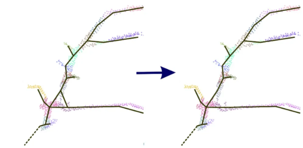
Figure 3: Skeleton generation. The background is the clustering result and the dash line means the branch connected to the root. Left: graph generated by connecting centers of neighboring clusters, which includes a loop in branching region (the triangle formed by three neighboring clusters). Right: skeleton generated by convert this graph into a tree. All the edges that do not belong to the shortest paths to the root cluster are removed.

3.3

Branch identification

Once the skeleton of the tree is computed, identifying all the branches becomes nec-essary for a tree modeling and simulation system. We propose a simple and intuitive method for detecting longest possible branches, which we call distance based method. A branch is defined as a sequence of nodes, which starts from a node of intersecting branches, i.e. the valence of the node val(Ni) ≥ 3 and ends with a leaf node. The main

trunk starts from the root, which is a special case. To identify all the branches, we first detect the main trunk of tree, then identify all the other branches recursively.

Starting from the root node, we first compute the longest distance for each node to the leave nodes recursively. We select the longest path as the main branch, and the other branches are detected recursively as following.

Detection of a branch is finished when a leaf node is reached. We use an FIFO queue to facilitate the branch detection procedure. The queue is initialized by pushing the root in the queue. The node on the top of queue is popped out repeatedly, and a branch with longest distance from this node to a leave node is detected. Each time when we find a branch, we check all the children of each node of this branch. If all the children of the node are already assigned to a branch, then this node is flagged as inactive, otherwise it is marked as active and pushed to the end of queue. The algorithm ends when the queue is empty. Algorithm 3.1 outlines the algorithm. The branch identification result of the apple tree is shown in Fig. 1 (middle right).

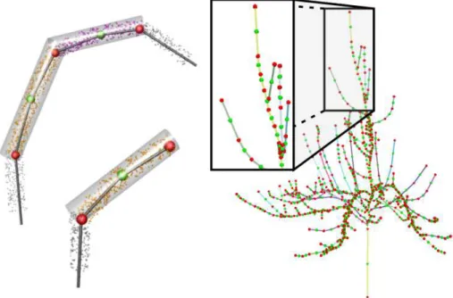
Figure 4: Definition of junction points. Upper left: the green spheres represent the center of each cluster, and the red spheres represent the internal junction points. Lower left: junction point definition of leaf node. Right: Skeleton generated by our method with junction points.

4

Tree modeling

The final step of our pipeline aims at providing a compact and smooth surface represen-tation of tree models not only for visualization but also for modeling and simulation, since further processing of tree models include intersection, self intersection, curvature or distance computation. We use the B-spline surface representation.

The B-spline surface not only offers high accuracy of representation but also sup-ports interactive shape manipulation by a designer using the B-spline control points. Another important advantage of the B-spline representation is that it comes together with a bunch of tools that allow to make it grow. This is especially useful when biolo-gists want to simulate e.g. the growth of trees.

The modeling of the tree is performed in two steps. First, the skeletons of tree branches are transformed into a set of B-spline curves. Second, these B-spline curves are used as paths to generate surface patches in a process called lofting [?].

4.1

B-spline fitting

The reconstruction step provides us with a structural description of the input data set that will serve as input to the modeling phase. Following this description, the output model will be a set of B-spline surface patches for all the branches of the tree.

Algorithm 3.1: Branch identification algorithm. Input: S, the skeleton of the tree

Output: B, the set of branches of the tree Create a queue Q ;

Q ← root(S) ; whileQ 6= ∅ do

Create a branch b ; Node t = pop(L) ; Node c = t ;

b← c ;

while !leaf(n=next(c)) do c= n ; b← c ; end foreach n∈ b do foreach c∈ children(b) do if !selected(c) then Q ← n ; end end B ← b ; end returnB ;

First, we fit a B-spline curve to the set of vertices of a branch skeleton. Recall that a vertex is either the center of a cluster or a junction point on the skeleton.

Given a set of m data points, {p1, . . . ,pm}, we compute a B-spline curve of order 4

(i.e. degree 3) with uniform knots and n control points to approximate all the skeleton vertices in the given order, and express this curve as

c(t) = n

∑

4.2

B-spline lofting

After we have obtained a B-spline curve as the central path, the radii of a tree branch along its central path can be obtained by linearly interpolating the radii of the bounding cylinders along its skeleton. Next we will explain how to use the lofting technique to define the control point of a B-spline sweep surface approximating a tree branch from the control points of the B-spline central path and the radius information of the branch. First we sample a sequence of n points vi on the central path c(t) and construct

normal planes Niof c(t) passing through the point vi. Here n is a user-specified

param-eter. On each plane Ni, we need to define a 2D local ortho-normal coordinate frame

Fi with the vi as the origin such that the sequence of the frames Fi exhibits no twist

about the central curve of the tree branch. We compute these frames using the method in [WJZL08] for computing a rotation minimization frame (RMF).

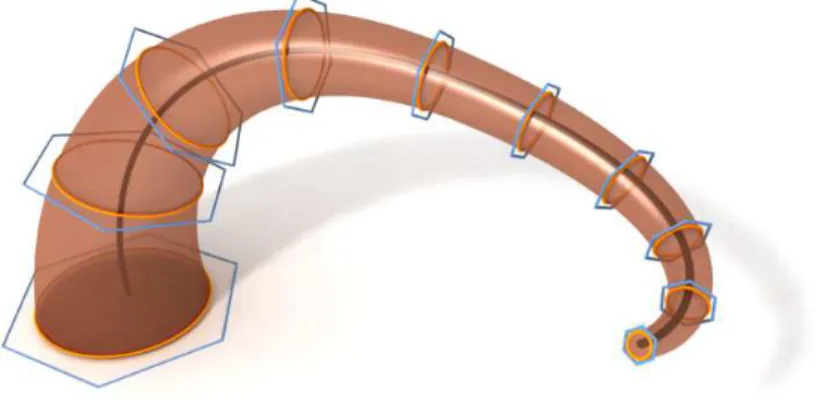
Then on each plane Ni, we position a regular polygon Hiwith fixed orientation with

respect to the frames Fion the successive planes Ni, as shown in Fig. 5. Here the size of

the polygon on each plane Niis scaled by the radius of the tree branch that we computed

earlier. Denote the vertices of the polygon Hi by ci, j, i = 1,2,...,n1, j = 1,2,...,n2.

We choose n2= 10 in our implementation. Then we obtain a tensor product B-spline

surface s(u, v) = n1

∑

∑

Fig. 5 shows the process of lofting operation.

We note that the use of rotation minimization frame (RMF) here is critical to the quality of the B-spline surface representation, since the commonly used Frenet frame is unstable on a general curve in 3D; for instance, its normal vector flips at inflection points of the central path [WJZL08].

Figure 5: Illustration of lofting operation.

5

Results and discussion

Model |P| |C| |B| Segmentation Branching Modeling hetre 34542 80 26 5.94 0.015 1.1 apple tree 60126 356 96 26.5 0.048 6.6 melgueil 117601 370 103 73.4 0.078 9.255

walnut 217187 1394 502 215.2 1.034 114.4 Table 1: Timing Statistics in seconds. |P| is the number of points obtained from the scan, |C| is the number of computed clusters and |B| is the number of branches. Seg-mentation, branching and modeling are the time taken by clustering, branch reconstruc-tion and B-spline lofting, respectively.

This work has been implemented as a plugin in the algebraic geometric modeling environment, which allows the visualization and manipulation of geometric objects with algebraic representation such as implicit or parametric curves or surfaces.

The input point cloud is normalized into the unit cube [0,1]3 _{at the initialization}

stage. The threshold ε for clustering is set to 1e−5_{and the maximal number of iterations}

is set to 30 in all our experiments (Section 2.2). The error threshold δ (Section 2.3) is different for models with different noise level, which varies in the interval [1e−3

,1e−2]. Fig. 1, 2, 3 and 4 give the detailed description of each step in our modeling process.

Fig. 6 shows a testing result on a noisy model which is not well aligned after multi-view scan. Our algorithm can still produce a result which is similar to its original structure. More testing results of complex models are given in Fig. 7 and Fig. 8.

Figure 6: Reconstruction result of fagus. Top: Segmentation and branch detection result. Bottom: Skeleton and the lofting result.

Table 1 lists the timing statistic of our algorithm tested on various scanned point mod-els. The lofting time depends on the number of sample points used to create the B-spline surface. The default number is 30.

Firstly, they compute shortest paths on input point data directly. Then all the points are clustered into bins after quantification of the shortest distance to the root. This does not consider any geometric information of the input data. In contrast, our variational segmentation approach tries to isolate the cylindrical regions from input data, and we compute the shortest paths for segmented clusters, which is more efficient. We also introduce junction points for skeleton extraction, which yield better results than only use the centers of each cluster, as shown in Fig. 3. In addition, the branch structure is constructed from the skeleton, which is needed by tree grown simulation. A com-parison of generated skeleton of Xu et al. ’s method and ours is given in Fig. 9, which indicates that, using the same number of clusters, our method yields a more efficient and more faithful representation of a reconstructed tree.

6

Summary and outlook

In this paper, we present an efficient framework for reconstructing ramified tree struc-ture from scanned point cloud data. Our segmentation algorithm is simple and easy to implement. The whole process is automatic but can also be dynamically controlled by the user easily. The result model can be used not only for simulation but also for rendering. The output branches can easily be converted into a piecewise linear mesh representation by sampling the B-spline representation of our surface patches. How-ever, the algebraic representation we provide has important applications in many fields such as agronomy and botany, enabling many algorithms to analyze the growth of trees in different stages. In the future, we plan to improve our reconstruction pipeline so that we could deal with the scanned point data with leaves.

References

[BB90] BLOOMENTHALJ., B.WYVILL: Interactive techniques for implicit

mod-eling. In Computer Graphics (Proceedings of Symposium on Interactive 3D Graphics)(1990), vol. 24(2), pp. 109–116.

[BMG06] BOUDON F., MEYER A., GODINC.: Survey on Computer

Representa-tions of Trees for Realistic and Efficient Rendering. Tech. Rep. RR-LIRIS-2006-003, Feb. 2006.

[BPF∗_{03] BOUDONF., PRUSINKIEWICZP., FEDERLP., GODINC., KARWOWSKI}

R.: Interactive design of bonsai tree models. In Computer Graphics Forum (Proceedings of Eurographics 2003)(2003), vol. 22(3), pp. 591– 599.

[CAD∗_{ar] CHAMBELLANDJ., ADAMB., DONÉSN., BALANDIERPH. MARQUIER}

A., DASSOT M., SONOHATG. SAUDREAUM., SINOQUET H.:

Auto-matic instantiation of a structural leaf model from 3D scanner data: ap-plication to light interception computation. Functinal Plant Biology (to appear).

[CSAD04] COHEN-STEINER D., ALLIEZP., DESBRUNM.: Variational shape

ap-proximation. ACM Transactions on Graphics 23, 3 (2004), 905–914. [Gär99] GÄRTNERB.: Fast and robust smallest enclosing balls. In Annual

Euro-pean Symposium on Algorithms (ESA)(1999), vol. 1643, pp. 325–338. [GCS99] GODIN C., COSTES E., SINOQUET H.: A method for describing plant

architecture which integrates topology and geometry. Annals of Botany 84 (1999), 343–357.

[GP04] GORTEB., PFEIFERN.: Structuring laser-scanned trees using 3D

math-ematical morphology. In Proceedings of 20th ISPRS Congress (2004), pp. 929–933.

[HB03] HART J. C., BAKER B.: Structural simulation of tree growth and

re-sponse. The Visual Computer 19, 2-3 (2003), 151–163.

[IOI06a] IJIRIT., OWADAS., IGARASHIT.: Seamless integration of initial sketch-ing and subsequent detail editsketch-ing in flower modelsketch-ing. Computer Graphics Forum 25, 3 (2006), 617–624.

[IOI06b] IJIRI T., OWADA S., IGARASHIT.: The sketch l-system: Global con-trol of tree modeling using free-form strokes. In Smart Graphics (2006), pp. 138–138.

[Llo82] LLOYDS.: Least square quantization in PCM. IEEE Trans. Inform Theory

28(1982), 129–137.

[MA06] MOUNTD. M., ARYAS.: ANN: A library for approximate nearest

neigh-bor searching, 2006.

[NFD07] NEUBERT B., FRANKEN T., DEUSSEN O.: Approximate image-based

tree-modeling using particle flows. ACM TOG 26, 3 (2007), Article 88. [OOI05] OKABE M., OWADA S., IGARASH T.: Interactive design of

botani-cal trees using freehand sketches and example-based editing. Computer Graphics Forum 24, 3 (2005), 487–496.

[PGW04] PFEIFERN., GORTEB., WINTERHALDERD.: Automatic reconstruction of single trees from terrestrial laser scanner data. In In Proceedings of 20th ISPRS Congress(2004), pp. 114–119.

[PH02] PYYSALOU., HYYPPH.: Reconstructing tree crowns from laser

scan-ner data for feature extraction. In Proceedings of ISPRS Commission III (2002), pp. 218–221.

[PHHM97] PRUSINKIEWICZP., HAMMELM., HANANJ., MECHR.: Visual models

[PS05] PHATTARALERPHONGJ., SINOQUETH.: A method for 3d reconstruction

of tree crown volume from photographs: assessment with 3D-digitized plants. Tree Physiology 25 (2005), 1229–1242.

[QTZ∗_{07] QUAN L., TAN P., ZENG G., YUAN L., WANG J., KANG S.:}

Image-based plant modeling. ACM TOG 25, 3 (July 2007), 599–604.

[RMD04] RECHE A., MARTINI., DRETTAKISG.: Volumetric reconstruction and

interactive rendering of trees from photographs. ACM TOG 23, 3 (2004). [SRDT01] SHLYAKHTER I., ROZENOER M., DORSEY J., TELLER S.:

Recon-structing 3D tree models from instrumented photographs. IEEE Computer Graphics and Applications 21, 3 (2001), 53–61.

[SRG97] SINOQUET H., RIVET P., GODIN C.: Assessment of the

three-dimensional architecture of walnut trees using digitising. Silva Fennica 31, 3 (1997), 265–273.

[TCH07] TENGC.-H., CHENY.-S., HSUW.-H.: Constructing a 3D trunk model from two images. Graphical Models 69, 1 (January 2007), 33–56. [TZW∗_{07] TAN P., ZENG G., WANG J., KANG S., L.QUAN: Image-based tree}

modeling. ACM TOG 26, 4 (2007), 303–308.

[WJZL08] WANG W., JÜTTLERB., ZHENG D., LIU Y.: Computation of rotation

minimizing frame. ACM TOG 27, 1 (2008), 2:1–2:18.

[WP95] WEBERJ., PENNJ.: Creation and rendering of realistic trees. ACM TOG

3(1995), 119–128.

[XGC07] XUH., GOSSETTN., CHENB.: Knowledge and heuristic-based

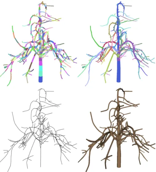
Figure 7: Reconstruction result of melgueil. Top: Segmentation and branch detection result. Bottom: Skeleton and the lofting result.

Figure 8: Reconstruction result of walnut. Top: Segmentation and branch detection result. Bottom: Skeleton and the lofting result.

Figure 9: Comparison of skeleton results. The background is the clustered point data overlayed with the skeleton. Left: Skeleton generated by Xu et al.’s method with 357 clusters. Right: skeleton of our method with 356 clusters. Our method produces a better clustering and produces geometric details more faithfully.