HAL Id: hal-01805246
https://hal.archives-ouvertes.fr/hal-01805246
Submitted on 8 Oct 2020
HAL is a multi-disciplinary open access
archive for the deposit and dissemination of
sci-entific research documents, whether they are
pub-lished or not. The documents may come from
teaching and research institutions in France or
abroad, or from public or private research centers.
L’archive ouverte pluridisciplinaire HAL, est
destinée au dépôt et à la diffusion de documents
scientifiques de niveau recherche, publiés ou non,
émanant des établissements d’enseignement et de
recherche français ou étrangers, des laboratoires
publics ou privés.
measurement network for estimating the biogenic CO2
budget of Europe
N. Kadygrov, G. Broquet, F. Chevallier, L. Rivier, C. Gerbig, P. Ciais
To cite this version:
N. Kadygrov, G. Broquet, F. Chevallier, L. Rivier, C. Gerbig, et al.. On the potential of the ICOS
atmospheric CO2 measurement network for estimating the biogenic CO2 budget of Europe.
At-mospheric Chemistry and Physics, European Geosciences Union, 2015, 15 (22), pp.12765 - 12787.
�10.5194/acp-15-12765-2015�. �hal-01805246�
www.atmos-chem-phys.net/15/12765/2015/ doi:10.5194/acp-15-12765-2015
© Author(s) 2015. CC Attribution 3.0 License.
On the potential of the ICOS atmospheric CO
2
measurement
network for estimating the biogenic CO
2
budget of Europe
N. Kadygrov1, G. Broquet1, F. Chevallier1, L. Rivier1, C. Gerbig2, and P. Ciais1
1Laboratoire des Sciences du Climat et de l’Environnement, CEA-CNRS-UVSQ, 91191, Gif sur Yvette CEDEX, France 2Max Planck Institute for Biogeochemistry, Jena, Germany
Correspondence to: N. Kadygrov (kadygrov@gmail.com)
Received: 8 December 2014 – Published in Atmos. Chem. Phys. Discuss.: 20 May 2015 Revised: 26 October 2015 – Accepted: 28 October 2015 – Published: 18 November 2015
Abstract. We present a performance assessment of the Eu-ropean Integrated Carbon Observing System (ICOS) atmo-spheric network for constraining European biogenic CO2 fluxes (hereafter net ecosystem exchange, NEE). The per-formance of the network is assessed in terms of uncertainty in the fluxes, using a state-of-the-art mesoscale variational atmospheric inversion system assimilating hourly averages of atmospheric data to solve for NEE at 6 h and 0.5◦ reso-lution. The performance of the ICOS atmospheric network is also assessed in terms of uncertainty reduction compared to typical uncertainties in the flux estimates from ecosystem models, which are used as prior information by the inver-sion. The uncertainty in inverted fluxes is computed for two typical periods representative of northern summer and win-ter conditions in July and in December 2007, respectively. These computations are based on a observing system simu-lation experiment (OSSE) framework. We analyzed the un-certainty in a 2-week-mean NEE as a function of the spatial scale with a focus on the model native grid scale (0.5◦), the country scale and the European scale (including western Rus-sia and Turkey). Several network configurations, going from 23 to 66 sites, and different configurations of the prior un-certainties and atmospheric model transport errors are tested in order to assess and compare the improvements that can be expected in the future from the extension of the network, from improved prior information or transport models. Assim-ilating data from 23 sites (a network comparable to present-day capability) with errors estimated from the present prior information and transport models, the uncertainty reduction on a 2-week-mean NEE should range between 20 and 50 % for 0.5◦ resolution grid cells in the best sampled area en-compassing eastern France and western Germany. At the
Eu-ropean scale, the prior uncertainty in a 2-week-mean NEE is reduced by 50 % (66 %), down to ∼ 43 Tg C month−1 (26 Tg C month−1) in July (December). Using a larger net-work of 66 stations, the prior uncertainty of NEE is reduced by the inversion by 64 % (down to ∼ 33 Tg C month−1) in July and by 79 % (down to ∼ 15 Tg C month−1) in December. When the results are integrated over the well-observed west-ern European domain, the uncertainty reduction shows no seasonal variability. The effect of decreasing the correlation length of the prior uncertainty, or of reducing the transport model errors compared to their present configuration (when conducting real-data inversion cases) can be larger than that of the extension of the measurement network in areas where the 23 station observation network is the densest. We show that with a configuration of the ICOS atmospheric network containing 66 sites that can be expected on the long-term, the uncertainties in a 2-week-mean NEE will be reduced by up to 50–80 % for countries like Finland, Germany, France and Spain, which could significantly improvement (and at least a high complementarity to) our knowledge of NEE derived from biomass and soil carbon inventories at multi-annual scales.
1 Introduction
Accurate information about the terrestrial biogenic CO2 fluxes (hereafter net ecosystem exchange – NEE) is needed at the regional scale to understand the drivers of the carbon cycle (Ciais et. al., 2014). Accounting for the natural fluxes in political agreements regarding the reduction of the CO2 emissions requires their accurate quantification over
admin-istrative areas, and in particular over countries and smaller regional scales at which land management decisions can be implemented.
Atmospheric inversions, which exploit atmospheric CO2 mole fraction measurements to infer information about sur-face CO2 fluxes (Enting, 2002) are expected to deliver ro-bust and objective quantification of NEE at high temporal and spatial resolution over continuous areas and time peri-ods. Global atmospheric inversions have been widely used to document natural carbon sources and sinks (Gurney et al., 2002; Rödenbeck et al., 2003). However, the spread of the results from the different global inversion studies and the di-agnostics by some of these studies demonstrates that the un-certainties remain large at the 1 month and continental scale (Peylin et al., 2013). Such large uncertainties are mainly due to the lack of observations over the continents or to the lim-ited ability of global systems to account for dense obser-vation networks in addition to errors in large-scale atmo-spheric transport models. However, with an increasing num-ber of continuous atmospheric CO2observations, primarily in North America and Europe, and with the development of regional inversion systems using high-resolution mesoscale atmospheric transport models and solving for NEE at typical resolutions of 10 to 50 km (Lauvaux et al., 2008, 2012; Schuh et al., 2010; Broquet et al., 2011; Meesters et al., 2012), there is an increasing ability to constrain NEE at continental to re-gional scales.
This paper aims at studying the skill of a regional inversion system in Europe, which is equipped with a relatively large number of ground-based atmospheric measurement stations, for estimating NEE at the continental and country scales, down to 0.5◦resolution (which is the resolution of the
trans-port model used in the inversion system). It also aims at as-sessing and comparing the benefits from the measurement network extensions and from future improvement in the in-version system. Such an improvement can be anticipated ei-ther due to better atmospheric transport models or to the use of better flux estimates as the prior information that gets up-dated by the inversion based on the assimilation of atmo-spheric measurements.
Europe is a difficult application area for atmospheric inver-sion because of the very heterogeneous distribution of vege-tation types, land use, and agricultural and industrial activi-ties inside a relatively small domain, and, consequently, be-cause of the need for solving for fluxes at high resolution. Furthermore, its complex terrain also requires a high resolu-tion of the topography when modeling the atmospheric trans-port (Ahmadov et al., 2009). However, the Integrated Carbon Observing System (ICOS) infrastructure is setting up a dense network of standardized, long-term, continuous and high pre-cision atmospheric and flux measurements in Europe, with the aim of understanding the European carbon balance and monitoring the effectiveness of greenhouse gas (GHG) miti-gation activities (http://www.icos-infrastructure.eu/). The at-mospheric network is expected to increase from an initial
configuration of around 23 stations, where actual measure-ments have been conducted during the past 5 years (even though all these sites will not necessarily be included in the official ICOS network in the coming years), up to around 60 stations in the near future (see ICOS Stakeholder hand-book 2013 at https://icos-atc.lsce.ipsl.fr/?q=doc_public). In this context, the developers of the ICOS atmospheric network have encouraged network assessment studies such as the one conducted in this paper.
Several inversion studies have focused on the esti-mate of European NEE based on measurements from the CarboEurope-IP atmospheric stations, most of which are planning to join the ICOS atmospheric network (Peters et al., 2010; Broquet et al., 2011). Broquet et al. (2013) have demonstrated, based on comparisons with independent flux tower measurements, that there is a high confidence in the Bayesian estimate of the European NEE and of its uncer-tainty at the 1-month and continental scale based on their variational system, which uses the CHIMERE mesoscale transport model run at 0.5◦ resolution. The distributions of the misfits between 1-month- and continental-scale averages of the flux measurements and of the NEE estimates sampled at the flux measurement locations were shown to be unbiased and consistent with the estimate of the uncertainties from the inversion system. This gives confidence in the inversion con-figuration of Broquet et al. (2011, 2013) for the estimation of the performance of the ICOS network. In particular, it gives confidence in their assumptions that the distribution of the uncertainties is unbiased and Gaussian, and that the impact of the uncertainties in the CO2modeling domain boundary conditions at the edges of Europe and in the CO2fossil fuel emissions is weak, when assimilating measurements from the type of sites that form the ICOS network.
Here, we apply the system of Broquet et al. (2011, 2013) to assess the potential of the near-term and realistic fu-ture configurations of the ICOS continuous measurements of CO2 dry air mole fraction to improve NEE estimates at the mesoscale across Europe. This assessment is based on a quantitative evaluation of the uncertainties in the inverted fluxes (also called posterior uncertainties), which are com-pared to the uncertainties in the prior information on NEE used by the inversion system.
The Bayesian statistical framework chosen here provides estimates of the posterior uncertainties as a function of the prior uncertainties, of the atmospheric transport and of the combination of statistical errors, which are not controlled by the update of the prior NEE by the inversion (like the mea-surement errors and the atmospheric transport errors). Even though the prior uncertainty can potentially depend on the value of the prior NEE, the actual values of the prior NEE or of the measurement data to be assimilated are not formally involved in the estimation of the posterior uncertainty due to the linearity of the atmospheric transport of CO2. There-fore, the posterior uncertainty can be derived for hypothetical observation networks or for hypothetical uncertainties in the
prior information or from the atmospheric transport model (i.e., for hypothetical improvements in the prior information or in the atmospheric transport model) using an observing system simulation experiment (OSSE) framework, in which the results do not depend on a simulated truth. Due to the dimension of the problem, uncertainties are not derived an-alytically in this study and we use a Monte Carlo ensemble approach.
Using synthetic data in an OSSE framework has been a common way to assess the utility of new GHG observ-ing systems for the monitorobserv-ing of the GHG sources and sinks at large scales based on global inversion systems with coarse-resolution transport models (e.g., Rayner et al., 1996; Houweling et al., 2004; Chevallier et al., 2007; Kadygrov et al., 2009; Hungershoefer et al., 2010). This approach now plays a critical role in the recent emergence of regional in-version systems supporting strategies for the deployment of regional observation networks and assessing the potential of regional inversion for assessing the GHG fluxes at a rela-tively high resolution (Tolk et al., 2011; Ziehn et al., 2014). Such a use of OSSEs today is not specific to the GHG inver-sion community. The OSSEs are increasingly used by the air quality community (e.g., Edwards et al., 2009; Timmermans et al., 2009a, b, 2015; Claeyman et al., 2011) and they are still extensively used by the meteorological community (e.g., Masutani et al., 2010; Riishøjgaard et al., 2012; Errico et al., 2013; see also https://www.gmes-atmosphere.eu/events/ osse_workshop/).
In OSSEs, twin experiments are often used to derive a sin-gle realization of the uncertainties (Masutani et al., 2010) while our Monte Carlo approach explores the uncertainty space much more extensively. Further, in common (linear) CO2 atmospheric inversions, since the results are indepen-dent of the synthetic true data used for the OSSE, any simu-lation can be used to build this truth, while, when using fra-ternal twin experiments with nonlinear models in other ap-plication fields of data assimilation, it is critical to ensure that the truth is realistic enough (Halliwell et al., 2014). The reliability of the OSSEs in CO2atmospheric inversion crit-ically depends on the realism of their input error statistics because their configuration in the inversion system is per-fectly consistent with the sampling of synthetic errors that are used in these experiments. In this study, our confidence in the realism of the statistical modeling approach and of the input error statistics, and thus in the inversion setup, is based on the statistical modeling studies of Chevallier et al. (2012) and Broquet et al. (2013) that were themselves based on real data.
The manuscript first documents the potential of different configurations of the ICOS network for constraining NEE, through the use of a state-of-the-art inversion setup, which solves the NEE at high spatial and temporal resolution, and which has been submitted to a high level of evaluation. This inversion setup is based on a variational atmospheric inversion system. We study the potential of the 23 station
(hereafter ICOS23) network containing existing sites and other stations that could be installed on tall towers over Eu-rope in the coming years. We also consider two longer-term ICOS configurations with 50 stations (hereafter ICOS50) and 66 stations (hereafter ICOS66). For the time domain, we con-sider results for NEE aggregated at the 2-week scale, for two different periods of the year (in July and in Decem-ber). Shorter aggregation scales, like a day, result in a signifi-cant dependency of NEE on specific synoptic events. Longer timescales require computing resources that are beyond the scope of this study with its high-resolution inversion system. We pay special attention to the analysis of the results at dif-ferent spatial scales, from the native transport model grid scale of about 50 km × 50 km up to the national scale that is the most relevant for supporting environmental policy, and the full European domain considered in this study (which ex-tends to western Russia and Turkey). We also present the sen-sitivity of our results to parameters characterizing the future developments of mesoscale inversion systems: the reduction of the transport model errors or of the prior flux errors.
The paper is organized as follows. Section 2 describes the mesoscale inversion experimental framework focusing on the Monte Carlo estimate of uncertainties. Section 3 analyzes the scores of posterior uncertainties and the uncertainty reduc-tion compared to the prior uncertainties in order to assess the potential of the near-term framework and of future im-provements of the network or of the inversion setup. The last section synthesizes the results and discusses them.
2 Materials and methods
2.1 The configurations of the ICOS atmospheric observation network
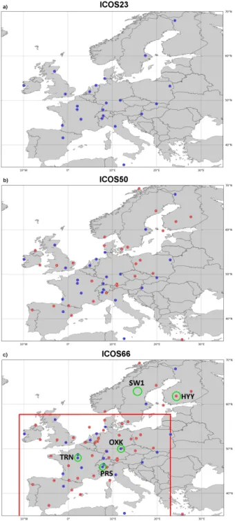
We consider three successive phases of deployment of the ICOS atmospheric network. The initial ICOS23 configura-tion includes 23 sites among which there are 10 tall towers. This minimum network configuration is based on existing stations, most of them being operational in the CarboEurope-IP FP6 project. The ICOS network is expected to further ex-pand during the next 5 years according to the country decla-rations at the ICOS Interim Stakeholder Council and to the ICOS European Research Infrastructure Consortium 5-year financial plan. Using possible locations for the future sta-tions, including sites that have already been discussed with the ICOS consortium during the ICOS preparatory phase FP7 project (European Union’s Seventh Research Frame-work Programme, grant agreement no. 211574), we derived two plausible ICOS configurations: ICOS50 with 50 sites in-cluding 27 tall towers and ICOS66 with 66 sites inin-cluding 39 tall towers.
The locations and details on the sites of the three configu-rations are summarized in Table A1 and in Fig. 1. Here, the existing and future ICOS CO2 observations are assumed to
Figure 1. Site location for the different ICOS network
configura-tions used in this study: (a) ICOS23, (b) and ICOS50 (c) ICOS66. Dark blue circles correspond to ICOS23 and the red circles are the new sites for ICOS50 and ICOS66 compared to ICOS23. The European domain (∼ 6.8 × 10⁶km2 of land surface) covered by these figures corresponds to the domain of the configuration of the CHIMERE atmospheric transport model used in this study. The red rectangle in panel (c) corresponds to a western European do-main (WE dodo-main, ∼ 3.5 × 10⁶km2of land surface), which is used for some of the present analysis because it is significantly better sampled by the ICOS networks than other areas. Green circles in panel (c) are the station locations used for the study of the uncer-tainty reduction as a function of the spatial scale of the aggregation around each station (in Sect. 3.1.4).
comply with the World Meteorological Organization (WMO) accuracy targets of 0.1 parts per million (ppm) measurement precision (WMO, 1981; Francey, 1998), so that the measure-ment error is negligible in comparison to the other type of errors that have to be accounted for in the inversion frame-work such as the model transport and representation errors (see their typical estimates in Sect. 2.2.2).
2.2 Mesoscale inversion system 2.2.1 Method
The estimate of uncertainties related to the different ICOS networks is based on an ensemble of inversions with the vari-ational inversion system of Broquet et al. (2011), assimilat-ing synthetic hourly averages of the atmospheric CO2data from these networks (during the afternoon or during night-time only, depending on the type of sites that are considered; see Sect. 2.2.2). A regional atmospheric transport model (see its description below) is used to estimate the relationship be-tween the CO2fluxes and the CO2mixing ratios. The inver-sion system solves for 6 h mean NEE on each grid point of the 0.5◦×0.5◦resolution grid used for the transport model-ing. It also solves for 6 h mean ocean fluxes at 0.5◦spatial resolution in order to account for errors from air–sea fluxes when mapping fluxes into hourly mean mixing ratios. How-ever, analyzing the uncertainty reduction for ocean fluxes is beyond the scope of this paper.
Peylin et al. (2011) indicate that uncertainties in anthro-pogenic fluxes yield errors when simulating CO2 mixing ratios at ICOS stations that are smaller than atmospheric model errors. Furthermore, the relative uncertainty in anthro-pogenic emissions is smaller than that in NEE, while on short timescales, the anthropogenic signal is generally smaller than the signature of the NEE at sites that are not very close (typically distances less than 40 km) to strong anthropogenic sources such as cities (see the analysis for the Trainou ICOS station near Orléans, France; Bréon et al., 2015). Relying on such indications, we assume that the errors due to un-certainties in anthropogenic emissions are negligible com-pared to errors from NEE and atmospheric model errors. This is a reasonable assumption as long as most ICOS sta-tions are relatively far from large urban areas, which should be the case because the ICOS atmospheric station specifi-cation document (https://icos-atc.lsce.ipsl.fr/?q=doc_public) recommends that the measurement sites be located at more than 40 km from the strong anthropogenic sources (such as the cities). Zhang et al. (2015) yielded conclusions from their transport experiments at 1◦resolution, which contradict this assumption and this clearly raises an open debate. However, the evaluation of the inversion configuration from Broquet et al. (2013) supports the use of this assumption for our study.
In order to simulate the full amount of CO2in the atmo-sphere, the inversion uses a fixed estimate of the fossil fuel emissions (see below) without attempting to correct it or
ac-count for uncertainties in these fluxes. The inversion also uses a fixed estimate of the CO2boundary conditions at the lateral and top boundaries of the regional modeling domain without attempting to correct it or account for uncertainties in these conditions. This follows the protocol from Broquet et al. (2011), which assumed that the error from the boundary conditions for the European domain is mainly bias and which corrects for such a bias in a preliminary step that is indepen-dent to the subsequent application of the inversion. Such an assumption is supported by the evaluation of the inversion configuration by Broquet et al. (2013). The relatively weak impact of uncertainties in the boundary conditions in Europe (while studies in other regions, such as that of Göckede et al., 2010, indicate a high influence of such uncertainties) can be explained by the fact that the spatial scale of the incoming CO2patterns at the ICOS sites from remote sources and sinks outside the European domain boundaries is relatively large compared to the typical distances between the ICOS sites, due to atmospheric diffusion (especially under west wind conditions, when the air comes from the Atlantic ocean). In principle, the inversion mainly exploits the smaller-scale sig-nal of the gradients between the sites to constrain the NEE, and it is thus weakly influenced by the large-scale signature of the uncertainty in the boundary conditions. In this section we only summarize the main elements of the inversion sys-tem, starting with the theoretical framework, while the de-tailed description can be found in Broquet et al. (2011).
We define the control vector x of the atmospheric inver-sion as the 6 h and 0.5◦×0.5◦mean NEE and ocean fluxes. The atmospheric inversion seeks the mean xaand covariance
matrix A of the normal distribution N (xa, A) of the
knowl-edge on x based on (i) the atmospheric transport model, (ii) the prior knowledge xbof x, (iii) the hourly mean
atmo-spheric measurements y, (iv and v) the covariances B and R of the distributions of the prior uncertainty and of the obser-vation error assuming that these uncertainties are normal and unbiased (i.e., equal to N (0, B) and N (0, R), respectively) and (vi) a Bayesian relationship between these distributions. The observation error is the combination of all sources of misfit between the atmospheric transport model and the con-centration measurements other than the prior uncertainty, in particular the measurement errors, the model transport, ag-gregation and representation errors, and the errors from the model inputs that are not controlled by the inversion.
With this theoretical framework, xais the minimum of the
quadratic cost function J (x) (Rodgers, 2000):
J (x) =1 2(x − xb) TB−1(x − x b) +1 2(H (x) − y) TR−1(H (x) − y) , (1) whereTdenotes the transpose, and where H is the affine ob-servation operator, which maps the 6 h (00:00–06:00, 06:00– 12:00, 12:00–18:00 and 18:00–24:00; UTC time is used hereafter) and 0.5◦×0.5◦mean NEE and ocean CO2fluxes
x to the observational space based on the linear CO2 at-mospheric transport model with fixed open-boundary con-ditions, and with fixed estimates of the anthropogenic fluxes and natural fluxes at resolutions higher than 6 h and 0.5◦. The operator H : x → H (x) can be rewritten H : x → Hx+yfixed, where yfixedis the signature, through atmospheric transport, of the fluxes (in particular the anthropogenic emissions) and boundary conditions not controlled by the inversion. The op-erator H is the combination of two linear opop-erators: the first operator distributing 6 h mean natural fluxes at the 1 h res-olution, and the second operator simulating the atmospheric transport from the 1 h resolution fluxes at 0.5◦resolution.
The inversion system derives an estimate of xa by
per-forming an iterative minimization of J (x) with the M1QN3 algorithm of Gilbert and Lemaréchal (1989). The gradient of J is derived using the adjoint operator of H thanks to the availability of the adjoint version of the CHIMERE code. The covariance of the posterior uncertainty in inverted NEE A, of main interest for this study, is given by the formula
A = (B−1+HTR−1H)−1. (2)
This equation demonstrates the point raised in the introduc-tion for justifying the OSSE framework; A does not depend on the observations or on the prior flux values themselves but only on their error covariance matrices, on the observation network density and station location, and on the atmospheric transport operator. This allows assessing the performance of any observation system, whether existing or not. Of note is also that this calculation does not depend on yfixed, i.e., on the boundary conditions or on the anthropogenic fluxes in the domain; therefore, such components can be ignored for the estimate of A.
In this framework, a common performance indicator is the theoretical uncertainty reduction for specific budgets of the NEE estimates (averaged over specified periods of time and over specified spatial domains), defined by
γ =1 −σa
σb
, (3)
where σa and σb are the standard deviations of the
poste-rior and pposte-rior uncertainties in the corresponding integrals in time and space (over the given periods of time and spatial domains) of the 6 h and 0.5◦resolution NEE field. If the ob-servations perfectly constrain the inversion of a given budget of NEE, then γ = 1. If the observations do not bring any in-formation to reduce the error from the prior, γ = 0. By defi-nition, γ is a quantity relative to the uncertainty in the prior fluxes, which depends on the type of prior information on NEE that is expected to be used (estimates from a biosphere model in our case, see Sect. 2.2.2). Of note is that the scores of uncertainty and of uncertainty reduction given in this study refer to the standard deviation of the uncertainty in a specific budget of NEE, and that, hereafter, the term standard
Due to the size of the observation and control vectors in this study, we could not afford the analytical computation of Eq. (2) based on the full computation of the H matrix (us-ing a very large number of transport simulations, as done in Hungershoefer et al. (2010). Instead we use the Monte Carlo approach of Chevallier et al. (2007) to compute A. In this ap-proach, an ensemble of posterior fluxes xaiis derived from an ensemble of inversions using the synthetic prior flux xbiand data yi, whose random errors (xbi-xtruefor xbiand yi-Hxtrue for yi) with respect to a known truth (xtrue, whose value does not influence the results analyzed here, and which is thus ig-nored hereafter) sample the distributions N (0, B) and N (0, R). A is obtained as the statistics of the posterior errors xai
-xtrue. The practical size of the ensemble is described below and its determination follows the discussion by Broquet et al. (2011). The convergence of the estimate of the inverted NEE for each inversion and the convergence of the statistics of the ensemble are necessary to ensure that the A matrix computed with this method corresponds to the actual covari-ance of the posterior uncertainty given by Eq. (2). These con-vergences cannot be perfect with a limited number of itera-tions for the minimization algorithm and a limited number of inversion experiments in the Monte Carlo ensemble imposed by computational limitations. Therefore, the estimate of A can depend on parameters other than H, B and R in practice, e.g., the number of iterations and of inversion experiments. However, it has been checked (see Sect. 2.2.2) that the con-vergence is sufficient, so that this dependence should not be significant for the quantities of interest.
2.2.2 Practical setup Atmospheric transport model
In this study, the operator H is based on the, CHIMERE mesoscale atmospheric transport model (Schmidt et al., 2001) forced with European Centre for Medium-Range Weather Forecasts (ECMWF) winds. We use a configuration with a 0.5◦×0.5◦horizontal grid and with 25 σ -coordinate vertical levels starting from the surface and with a ceiling at ∼ 500 hPa (such a ceiling being usual for regional trans-port modeling when focusing on mole fractions close to the ground, e.g., Marécal et al., 2015). The spatial extent of the corresponding domain is described below. CHIMERE is an off-line transport model. Hourly mass fluxes are provided by the ECMWF analyzes. The relatively high vertical and hor-izontal resolutions of CHIMERE allow for a good vertical discretization of the planetary boundary layer (PBL; the first 14 levels are below 1500 m) along with a good representa-tion of the orography and dynamics to match high frequency observations better than with a global configuration, whose typical horizontal resolution is ∼ 3◦(Peylin et al., 2013).
Spatial and temporal domains
In this study, we use the European domain shown in Fig. 1a, which covers most of the European Union and some of east-ern Europe, with a land surface area of 6.8 × 10⁶km2. Its southwest corner is at 35◦N and 15◦W, and its northeast cor-ner is at 70◦N and 35◦E. Two temporal windows are consid-ered, from 30 June to 20 July 2007 and from 2 to 22 Decem-ber 2007 (of almost 3 weeks each). The choice of these peri-ods of 3 weeks is a tradeoff between widening the scope of the study and computational burden. The Monte Carlo-based flux uncertainty reduction calculations require large comput-ing resources, while we test three different network configu-rations for two different months, and for different setups of the error covariance matrices. Indeed, 3-week experiments allow for retrieving information about uncertainties at the 2-week scale without being biased by edge effects, i.e., they al-low accounting for the impact of uncertainties from the days before the 14 targeted days and for the impact of the assimila-tion of measurements during the days after these 14 targeted days. The advection of CO2throughout Europe can last more than 3 days, but atmospheric diffusion ensures that the sig-nature at ICOS sites of the NEE during a 6 h window is gen-erally negligible after 3 days of transport (not shown). Thus, the windows 3–17 July and 5–19 December were chosen for analysis. We consider the results for July and December to be representative for the summer and winter seasons (using the name of the seasons for the Northern Hemisphere hereafter), allowing an analysis of seasonal variations of the flux uncer-tainty reduction. Choosing year 2007 for the period of the in-version only impacts the meteorological conditions (i.e., the impact on the prior uncertainty, whose local standard devia-tions are scaled using data from this specific year, as detailed below in this section, is negligible) and thus the atmospheric transport conditions in the OSSEs. We assume that these con-ditions are not impacted by a strong inter-annual anomaly in 2007 so that they can be expected to be representative of av-erage conditions for summer and winter. Hereafter, the men-tion of the year 2007 is thus often ignored and we assume that we retrieve typical estimates for July and December. Flux error covariance matrix
The setup of the error covariance matrix B follows the methodology of Chevallier et al. (2007). It is chosen to represent the typical uncertainty in estimates from the bio-sphere models (for NEE) and from climatologies (for ocean fluxes) used by traditional atmospheric inversion systems. The statistics have been derived for estimates from the Or-ganising Carbon and Hydrology In Dynamic Ecosystems (ORCHIDEE) vegetation model (Krinner et al., 2005) and the ocean climatology from Takahashi et al. (2009). The uncertainties in NEE are assumed to be autocorrelated in space and in time and are modeled using isotropic and expo-nentially decreasing functions with correlation lengths that
do not depend on the time or location. A Kronecker prod-uct of the matrices of temporal and spatial correlations is applied to define the correlations between uncertainties for different locations and time windows. The e-folding spa-tial and temporal correlation lengths are set according to the estimation of Chevallier et al. (2012) based on com-parison of the NEE derived by the ORCHIDEE model and eddy-covariance flux tower data, for our specific prior flux spatial and temporal resolution, i.e., 30 days in time and 250 km in space over land. NEE uncertainties for different 6 h windows of the day are not correlated, i.e., the tempo-ral correlations only apply to a given 6 h window of con-secutive days. The standard deviations of the prior uncer-tainties in B are set proportional to the heterotrophic respi-ration fluxes from the ORCHIDEE model (the correspond-ing proportional coefficient between the heterotrophic respi-ration and the prior uncertainty at the daily and 0.5◦scale is
approximately 2). We apply time-dependent scaling factors to these fluxes so that the NEE uncertainties have lower val-ues during the night than during the day, and during winter than during summer, providing typical values for grid scale and daily errors of ∼ 2.5 g C m−2day−1 in summer (maxi-mum value 3.4 g C m−2day−1) and of ∼ 2 g C m−2day−1in winter (maximum value 3.1 g C m−2day−1). Over the ocean, the prior uncertainty of air–sea fluxes has standard devia-tions at the 0.5◦and 6 h scale equal to 0.2 g C m−2day−1, an
e-folding spatial correlation length of 500 km and temporal
correlations similar to those for the prior uncertainties over land. Prior ocean and land flux uncertainties are not corre-lated.
Time selection of the data to be assimilated
Broquet et al. (2011) analyzed the periods of time during which the CHIMERE European configuration bears trans-port biases that are too high, so that measurements from ground-based stations such as ICOS sites should not be as-similated to avoid erroneously projecting such biases into the corrections to the fluxes. In agreement with common prac-tice, they concluded that observations at low altitude sites (approximately below 1000 m above sea level, m a.s.l.; see Broquet et al., 2011, for the exact definition of the differ-ent types of sites used for the time selection of the data and the configuration of the observation error), which include al-most all of the ICOS tall towers, should be assimilated dur-ing daytime (12:00–20:00) while the observations at high altitude stations (approximately above 1000 m a.s.l.) should be used only during the night (00:00–06:00). This generally yields larger uncertainty reduction during daytime than dur-ing nighttime (Broquet et al., 2011). However, this does not raise a potential bias related to a better constraint on day-time inverted NEE (when the ecosystems are generally a sink of CO2) than on nighttime inverted NEE (when the ecosys-tems are generally a source of CO2), since uncertainties in both nighttime and daytime prior NEE, transport and
mea-surements are assumed to be unbiased, as supported by the results from Broquet et al. (2013).
Observation error covariance matrix
The observational error covariance matrix R accounts for various sources of error when comparing the hourly data se-lected for assimilation and their simulation, which are not controlled by the inversion: measurement error, aggregation error, atmospheric model representativeness and transport error (as explained previously, uncertainties in the anthro-pogenic emissions and in the boundary conditions are as-sumed to be negligible). The first two terms are negligible compared to the model representativeness and transport er-ror due to the high measurement standard and to solving for the fluxes at 6 h and 0.5◦resolution during the inversion,
re-spectively.
Broquet et al. (2011) derived a quantitative estimation of the model error (depending on the station height) including transport and representativeness errors based on comparisons between simulations and measurements of CO2 and222Rn during summer. Broquet et al. (2013) extended this analy-sis using 1-year-long time series of simulated and measured CO2 and222Rn, to provide the season-dependent estimates that are used here. The model error is much higher during the winter than that during the summer. It is given for each site in Table A1 for the 2 months (July, December) considered in this study. We assume that the errors for two different sites are independent and that they do not bear temporal autocor-relations. Thus, the observation error covariance matrix R is set diagonal. There is no evidence that such autocorrelations could be significant in the analysis of Broquet et al. (2011). The resulting budget of observation errors at daily to monthly resolution is reliable (Broquet et al., 2011, 2013). This sug-gests that the temporal autocorrelations of the actual observa-tion errors are negligible. If the autocorrelaobserva-tions of the actual observation errors were not negligible, this would mean that the errors for hourly data are overestimated. In both cases, the assumption that the temporal autocorrelations of the ob-servation error are negligible does not seem to need to be balanced by an artificial increase of the estimate of the ob-servation errors for hourly averages provided by Broquet et al. (2013).
Minimization and number of members in the Monte Carlo ensembles
We use 12 iterations of minimization for each variational inversion of the Monte Carlo ensemble experiments. This number is similar to that from Broquet et al. (2011) where they considered a longer time period for the inversions but far smaller observation networks and a smaller inversion domain, which reduces the dimension of the minimization problem. However, here, 12 iterations were still found to be sufficient for converging toward the theoretical minimum of
the cost function, i.e., the number of assimilated data divided by 2 (Weaver et al., 2003), with less than 10 % relative differ-ence to this theoretical minimum except for a few cases (for these cases, 18 iterations were used to reach a relative differ-ence to the theoretical minimum that is smaller than 10 %).
Similarly to Broquet et al. (2011), 60 members are used in each Monte Carlo ensemble experiment. This is also the typ-ical number of members that Bousserez et al. (2015) used for their Monte Carlo simulations. Broquet et al. (2011) found a satisfactory convergence of the estimate of the uncertainties in Europe and 1-month-average NEE with an ensemble size of 60, which is confirmed here (the estimates using 50 and more members are within 6 % of the results with 60 mem-bers).
2.2.3 Sensitivity tests
Three and five Monte Carlo ensembles of inversions are con-ducted for December and July, respectively. For each season, three ensembles using the default setup of B and R described above are conducted in order to give results for the three different ICOS network configurations and consequently the sensitivity to the network configuration. In July, two ensem-bles are also conducted with a change in R in one case and in B in the other case in order to test the sensitivity to these inversion parameters. Such sensitivity tests were conducted in July only, using only one configuration of the ICOS net-work (ICOS50 and ICOS66 for the test of sensitivity to R and B, respectively); a more exhaustive set of tests of sensitivity for the two seasons and for each ICOS network configura-tion was not expected to bring new insights, but would raise significant additional computation costs. The setup of the in-version for these two sensitivity tests is now described. Test of the sensitivity to the observation error
There is a steady increase in the resolution of the atmospheric transport models used for atmospheric inversions, with cor-responding improvements of the simulation precision (e.g., Law et al., 2008). In this test we simulate the effect of po-tential future transport model improvement on the posterior flux uncertainties by reducing the default observation error standard deviations in R by a factor of 2. This factor roughly corresponds to the improvement of the misfits between the model and actual measurement at the site TRN (see Fig. 1 for its location), which was observed when bringing CHIMERE from the current 0.5◦ resolution down to a 2 km resolution
using the configuration presented in Bréon et al. (2015). The underlying assumption would be that ∼ 1 km horizontal res-olution atmospheric transport models could be used for in-versions at the European scale in the near future. Hereafter, we denote by Rref the reference configuration of R and by Rredthe one corresponding to reduced standard deviations.
Test of the sensitivity to the prior uncertainty
The test of the sensitivity of the inversion system to the prior uncertainty is focused on that of the sensitivity to the spatial correlation length in B (Gerbig et. al. 2006) (which impacts the budget of uncertainty over large regions). The possible use of better prior flux fields based on the merging of both estimates from vegetation models and from large-scale in-ventories (such as forest and agricultural inin-ventories) can be expected to generate smaller-scale uncertainties than when using vegetation models whereas it is not obvious that local uncertainties would be decreased when adding information from inventories (since inventories only measure long-term integrated NEE). Therefore, we tested the impact of reduc-ing the spatial correlation length for the prior uncertainty in NEE from 250 to 150 km, denoting hereafter the correspond-ing configurations for the B matrix: B250 and B150, respec-tively.
3 Results and discussion
3.1 Assessment of the performance of the actual network and system
In this section, the performance of the inversion relying on the default configuration and on the ICOS23 initial state net-work (i.e., the reference inversion) is analyzed as a function of the spatial scale, highlighting the main patterns of the un-certainty reduction obtained from the pixel scale to the re-gional (national, European) scales.
3.1.1 Analysis at the model grid scale
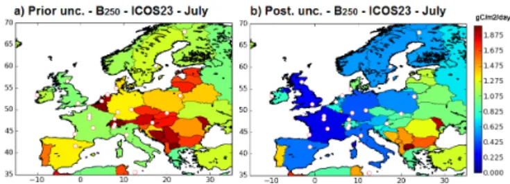
Figure 2a and b show the uncertainty reduction for estimates of a 2-week average NEE at 0.5◦resolution in July and De-cember, respectively. This grid-scale uncertainty reduction reaches 65 % for areas in the vicinity of the ICOS sites and decreases smoothly with distance away from measurement sites. For most of the area around eastern France–western Germany, this grid-scale uncertainty reduction ranges from 35 to 50 % for July and from 20 to 40 % for December. This stems from the combination of the dense observation net-work over that region, and from the 250 km correlation scale for the prior uncertainties, which spreads the error reduction beyond the immediate vicinity of each station where near-field fluxes have a large influence on the mixing ratio at this station (Bocquet, 2005). For other parts of Europe that are not well sampled by ICOS, significant uncertainty reductions are generally seen around each site but there are large areas where the inversion has no impact at the grid scale: Scandina-vian countries, the eastern part of Germany, Poland, the south of the Iberian Peninsula and almost all of eastern Europe.
The spatial structure of the uncertainty reduction and the underlying spatial extrapolation from a site is a complex combination of transport influence and of the structure of
Figure 2. Uncertainty reduction (theoretically comprised between
0 and 1) for a 2-week-mean NEE at 0.5◦resolution in July (a) and in December (b) when using ICOS23 (red dots) and the reference inversion setup. Red/blue colors indicate relatively high/low uncer-tainty reduction (with min = 0 and max = 0.68 in the color scale).
the prior uncertainty. Due to varying transport conditions, standard deviation of the prior uncertainty at the grid scale (which is larger in summer; see below the comments on Fig. 3), and observation error (which is larger in winter), the spatial distribution of uncertainty reduction is found to vary from summer to winter. Because the prior uncertainties are larger and the observation errors are smaller in July than in December, there is generally a larger uncertainty reduction in July (especially in western Europe). But variations in me-teorology alter (limiting or enhancing) this general behavior. The lower vertical mixing (which strengthens the sensitivity of the near-ground measurements to the local fluxes) partly balances the higher observation error in December and the range of local uncertainty reductions overlaps between July and December. The observations from the Angus tall tower (tta site, Table A1) in Scotland or from Pallas (pal site, Ta-ble A1) in Finland contribute differently to the uncertainty reduction during July and December (using meteorological conditions from 2007), showing better performance at the grid scale during summer. This also comes from the different weather regimes, with different dominant wind directions,
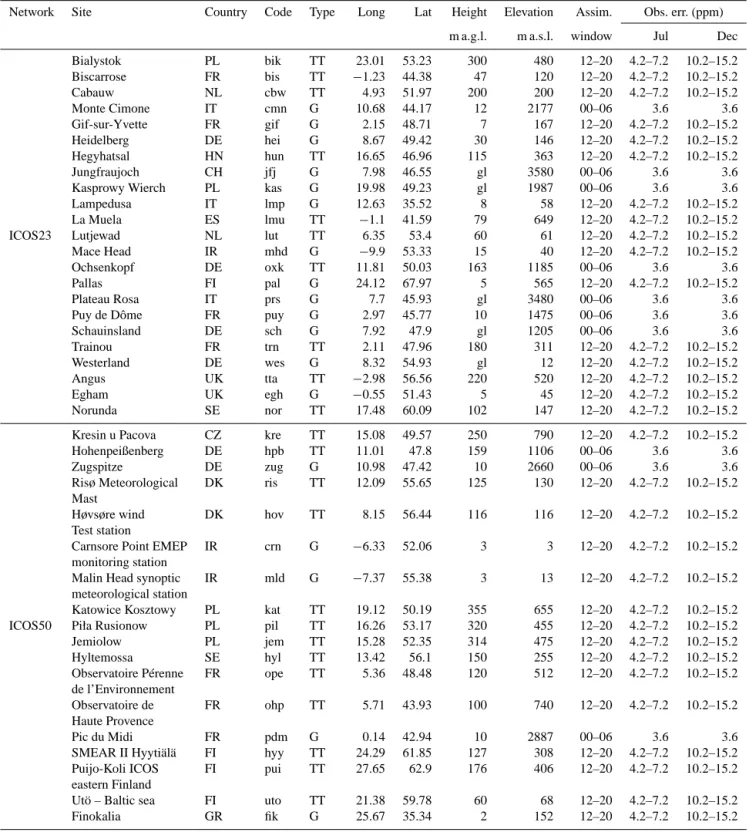
Figure 3. Standard deviations (g C m−2day−1) of the prior (a, b) and posterior (c, d) uncertainties in a 2-week-mean NEE at 0.5◦ res-olution for (a, c) July and (b, d) December. Posterior uncertainties are given for inversions using ICOS23 (red dots) and the reference inversion setup. Red/blue colors indicate relatively high/low uncer-tainties (with min = 0 g C m−2day−1and max = 3 g C m−2day−1 in the color scale).
different average wind speed and different vertical mixing in summer and winter. Regions lacking stations in ICOS23 have an uncertainty reduction that is more sensitive to the at-mospheric transport than regions with a dense network. The uncertainty reduction in December is significantly larger in the east and in the southeast part of domain compared to July, due to more occurrences of winds from the east during De-cember than during July.
Complementing the uncertainty reduction, Fig. 3 shows prior and posterior uncertainty standard deviations at the grid scale in order to illustrate the precision of the estimates of NEE that should be achievable with the reference inversion using the ICOS23 network. As already stated, prior uncer-tainties are up to ∼ 3 g C m−2day−1(Fig. 3a) but the winter values are smaller than the summer ones (due to a weaker activity of the ecosystems; Fig. 3b). During both July and December, the uncertainties in a 2-week-mean NEE in the regions that are best covered by observations (most of west-ern Europe) at 0.5◦ resolution are reduced by the inversion down to typical values of ∼ 1.5 g C m−2day−1(Fig. 3c, d). 3.1.2 Analysis at national scale
Figure 4a and b show the uncertainty reduction for a 2-week-and country-mean NEE in July 2-week-and December, respectively. The countries and corresponding estimates of prior and pos-terior uncertainties are listed in Table A2. The results suggest the ability of the mesoscale inversion framework to derive es-timates of the NEE at the national scales with relatively low uncertainties. The uncertainty reduction is particularly large for countries such as Germany, France and the UK, e.g., more than 80 % for France during July. It is larger than 50 % for a
Figure 4. Uncertainty reduction (theoretically comprised between 0
and 1) for a 2-week-mean NEE at the country scale for July (a) and December (b) when using ICOS23 and the reference inversion con-figuration. Red/blue colors indicate relatively high/low uncertainty reduction (with min = 0 and max = 0.95 in the color scale).
large majority of the countries in western Europe and Scan-dinavia both in July and December.
The smallest uncertainty reduction applies to southeast-ern European countries where it can be smaller than 10 % (e.g., for Greece in July) indicating that the presence of sta-tions very close to or within a given country is a requisite for bringing significant improvement to the estimates of NEE in this country. In general, the differences of the inversion skill between July and December look consistent with what has been analyzed at the pixel scale. In particular the uncertainty reduction is higher in July for western European countries but higher in December for eastern European countries for the same reasons as that given when analyzing the same be-havior at the pixel scale (see Sect. 3.1.1).
3.1.3 Analysis at the European scale
Table 1 shows that the uncertainty in a 2-week-mean NEE in July averaged over the full European domain (6.8 ×10⁶km2 of land surface) is reduced by the inversion by 50 % down to a value of ∼ 43 Tg C month−1(see Table 1 for details) us-ing the default configuration. The uncertainty reduction for
December is 66 %, resulting in a posterior uncertainty of
∼26 Tg C month−1. The uncertainty reduction for the whole European domain is thus higher in December than in July. More precisely, while easterly winds in December strongly favor this period in terms of uncertainty reduction in eastern Europe, the uncertainty reduction for NEE averaged over the reduced western European domain defined in Fig. 1c does not vary significantly with the season (66 and 64 % for July and December, respectively). This lack of seasonal variation in the uncertainty reduction at the scale of the western Euro-pean domain (where most of the ICOS23 stations are located) seems to contrast with the grid-scale and national-scale esti-mations in this domain, which indicates that the uncertainty reduction is generally significantly higher during summer than during winter. This contrast will be analyzed and in-terpreted in Sect. 3.1.4.
3.1.4 Analysis of the variations of the uncertainty as a function of the spatial aggregation of the NEE: interpretation of the results obtained at the national and European scales
In order to examine here the dependency of the NEE uncer-tainty reduction to increasing spatial scales of aggregation for the analyses in July and December, we choose five locations at which we define centered areas with increasing size for which uncertainties in the average NEE are derived. These stations are located using the green circles in Fig. 1c. The five locations correspond to three observing sites of ICOS23: Trainou (TRN), Ochsenkopf (OXK) and Plateau Rosa (PRS); one site of ICOS50: SMEAR II-ICOS Hyytiälä (HYY); and one point in Sweden, which does not correspond to any site of the ICOS networks tested here, called SW1 hereafter (Fig. 1c). We compute the uncertainty reductions of the 2-week-mean NEE for July and December over five squares centered around each site and of increasing size (in square degrees): 1.5◦×1.5◦, 2.5◦×2.5◦, 3.5◦×3.5◦, 4.5◦×4.5◦ and 10.5◦×10.5◦(which corresponds to surfaces of differ-ent size in terms of km2). Depending on their location and on their size, the corresponding domains expand over areas of Europe that are more or less constrained by the inversion at the pixel scale. But the variations of the uncertainty reduction when increasing the size of these domains are also strongly driven by the spatial correlations in the prior and posterior uncertainty. The results are displayed in Fig. 5.
The five locations used for this analysis are representa-tive of the diversity of the situation regarding the differences between grid scale uncertainty reduction in July and in De-cember. While the uncertainty reduction is slightly larger in July than in December for TRN and much larger in July for PRS and HYY, it is slightly larger in December at OXK and much larger in December at SW1. Furthermore, the values for these grid scale uncertainty reductions range from 15 to 50 % in July and from 7 to 47 % in December at these loca-tions (Fig. 5).
Table 1. Uncertainty reduction in a 2-week- and European-mean NEE for July and December as a function of the observation network and
of the configuration of the inversion parameters (B250or B150for B and Rrefor Rredfor R).
Month B R Prior uncertainty Posterior uncertainty NEE from ORCHIDEE Uncertainty (Tg C month−1) (Tg C month−1) (Tg C month−1) reduction (%)
ICOS23 July B250 Rref 91.2 42.6 −201.6 53
December B250 Rref 74.9 25.5 80.3 66 ICOS50 July B250 Rref 91.2 32.4 −201.6 64 December B250 Rref 74.9 19.5 80.3 74 July B250 Rred 91.2 30.4 −201.6 67 ICOS66 July B250 Rref 91.2 32.8 −201.6 64 December B250 Rref 74.9 15.4 80.3 79 July B150 Rref 55.0 29.2 −201.6 47
Figure 5. Uncertainty reduction (theoretically comprised between
0 and 1) for a 2-week-mean NEE in July and December 2007 us-ing ICOS23 and the reference configuration of the inversion, as a function of the size (logarithmic scale) of the spatial averaging area (in km2; as indicated by the crosses, for each curve values are derived for 1.5◦×1.5◦, 2.5◦×2.5◦, 3.5◦×3.5◦, 4.5◦×4.5◦and 10.5◦×10.5◦areas, which correspond to different values in terms of km2depending on their location in Europe) around each station: TRN (red curves), PRS (blue curves), HYY (green curves), OXK (pink curves) and SW1 (grey curves; see the locations in Fig. 1c). Solid and dash lines correspond to results for July and December, respectively (see the legend within the figure). The results of uncer-tainty reduction for the whole European domain are included (red rectangles). The results for the western European domain defined in Fig. 1c are included on curves corresponding to sites that are located in this domain (TRN, PRS and OXK; see the green rectangles).
The maximum scores of uncertainty reduction occur for spatial scales of aggregation ranging from 105 to 106km2 when considering the sites located in western Europe. These scales approximately correspond to the range of the sizes of the European countries and it is larger than the typical area of correlation of the prior uncertainty (as defined by prior cor-relation lengths of 250 km). Increasing the spatial resolution generally increases the uncertainty reduction since posterior
uncertainties have generally smaller correlation lengths than prior uncertainties, due to the spatial attribution error when trying to link the measurement information to local fluxes despite the atmospheric mixing. This explains the increase of uncertainty reduction from the grid scale to the national scales. This also explains why, for a given regional density of the measurement network, larger countries bear larger un-certainty reductions (Fig. 4). However, above such national scales, the corresponding domains include parts of eastern Europe being poorly sampled by the ICOS23 network, which explains the decrease in uncertainty reduction.
The convergence between the results around TRN, PRS and OXK in December and July (which tend to nearly 65 % uncertainty reduction when the averaging area reaches the western European domain), between the results around all sites in December (which tend to 66 % uncertainty reduction when the averaging area reaches the whole of Europe) or be-tween the results around all sites in July (which tend to nearly 53 % uncertainty reduction when the averaging area reaches the whole of Europe), starts between the 105 and 106km2 (national scale) averaging areas. For smaller areas, the dif-ferences between results in July and December or between results for different spatial locations stay similar to what is seen at the 0.5◦×0.5◦scale.
The similarity of the results for the western European do-main despite differences at the grid scale in July and De-cember can be explained by differences of correlations be-tween areas at scales similar to or larger than the national scale in the posterior uncertainties (since the correlations of the prior uncertainties aggregated at the national scale or at larger scales are very close for July and December). Figure 6 illustrates the variations of such correlations of the posterior uncertainty at the national scale between July and Decem-ber using the example of correlations between Germany and other countries. These correlations are usually more negative in December, which indicates a larger difficulty in December than in July to distinguish in the information from the mea-surement network the separate contributions of the different neighboring countries (or of different areas of larger size).
Figure 6. Correlations of the posterior uncertainties in a
2-week-mean NEE between Germany and the other European countries in July (a) and December (b) from the reference inversions with ICOS23. Germany is masked in white. Red/blue colors indicate rel-atively high positive/negative correlations (with min = −0.45 and max = 0.45 in the color scale).
This can be attributed to the stronger winds in December, which increase the extent of the flux footprints of the con-centration measurements. Such an increase of the footprints in December limit the ability to solve for the fluxes in the vicinity of the measurement sites but increase the ability to solve for the fluxes at large scales.
3.2 Impact of the extension of the ICOS network The effect on local (grid scale) uncertainty reduction of as-similating data from new sites in the ICOS network depends on the coverage of the area by the initial ICOS23 network, as illustrated by the comparison of the results using ICOS23, ICOS50 and ICOS66 and the reference configuration of the inversion (see Figs. 2 and 7). For example, adding one new site in Sweden or Finland yields a stronger increase of the un-certainty reduction than adding one site in the central part of western Europe, where the network is already rather dense. Since most of the new sites from ICOS23 to ICOS50 and then ICOS66 are located in western Europe, the improve-ments due to adding 27 or 43 sites to ICOS23 do not thus appear to be as critical as what can been achieved using the 23 sites of ICOS23. The changes from ICOS23 to ICOS50 significantly enhance the uncertainty reduction at 0.5◦ reso-lution in western Europe in July, e.g., with uncertainty reduc-tion increased from ∼ 40 % using ICOS23 to ∼ 60 % using ICOS66 in Switzerland. The impact of adding new sites is larger in December than in July, and, consequently, results for western Germany and Benelux converge between July and December when increasing the network to ICOS66.
The impact on the scores of uncertainty reduction of the increase of the ICOS network is also significant at the na-tional (cf. Figs. 4 and 8) and European scales (see Table 1 and Fig. 9) when comparing results with ICOS50 or ICOS66 to those obtained with ICOS23. The ICOS66 network de-livers uncertainty reductions as high as 80 % for countries like France and Germany in July. For Europe, the uncer-tainty reduction when using ICOS66 reaches 79 % down to
∼15 Tg C month−1posterior uncertainty in December, and
Figure 7. Uncertainty reduction (theoretically comprised between 0
and 1) for a 2-week-mean NEE at 0.5◦resolution in July (a, b) and December (c, d) when using ICOS50 (a, c) and ICOS66 (b, d) and the reference inversion configuration. Red dots corresponds to the ICOS23 (a, c) or ICOS50 (b, d) sites while white dots correspond to the additional sites included in ICOS50 or ICOS66, respectively. Red/blue colors indicate relatively high/low uncertainty reduction (with min = 0 and max = 0.68 in the color scale).
Figure 8. Uncertainty reduction (theoretically comprised between
0 and 1) for a 2-week-mean NEE at the country scale in July (a, b) and December (c, d), when using ICOS50 (a, c) and ICOS66 (b, d). Red/blue colors indicate relatively high/low uncertainty reduction (with min = 0 and max = 0.95 in the color scale).
64 % down to ∼ 33 Tg C month−1 posterior uncertainty in July. However, the increase from ICOS50 to ICOS66 does not seem to impact much the uncertainty reduction at these scales, especially in July.
Figure 9 illustrates the diversity (depending on the space locations) of the evolution of the impact of increasing the net-work as a function of the NEE averaging spatial scale. For a low altitude site already present in the dense part of ICOS23, the impact of adding new sites increases when increasing the
Figure 9. Uncertainty reduction (theoretically comprised between
0 and 1) for a 2-week-mean NEE for July 2007 as a function of the size (in logarithmic scale) of the spatial averaging area (same as for Fig. 5) centered on (a) SW1, (b) HYY, (c) TRN, (d) OXK, and (e) PRS. Red, orange and green lines: results with the reference configuration of the inversion using ICOS23, ICOS50 and ICOS66, respectively; blue: results when using ICOS50 and the inversion configuration with R = Rred; pink: results when using ICOS66 and the inversion configuration with B = B150. The results of uncer-tainty reduction for the whole European domain are included sys-tematically. The results for the western European domain defined in Fig. 1c are included on curves corresponding to sites, which are located in this domain (TRN, PRS and OXK).
spatial scale of the analysis up to areas where ICOS23 is less dense (mainly in eastern Europe) and where new sites are in-cluded in ICOS50. Conversely, the impact of the addition of new sites can decrease when increasing the NEE spatial ag-gregation scale, e.g., at HYY where a new site is specifically added in ICOS50.
3.3 Sensitivity to the correlation length of the prior uncertainty
The impact of reducing the correlation e-folding length (from 250 to 150 km) of the prior uncertainty in the inversion configuration is tested using ICOS66 in July (cf. Figs. 7b and 10a, Figs. 8b and 11a, and the corresponding curves in Fig. 9). Such a change of correlation length strongly decreases the values of uncertainty reduction at all spatial scales. This is because it decreases the prior uncertainty at every scale while decreasing the ability of the inversion sys-tem to extrapolate in space the information from measure-ment sites based on the knowledge of spatial correlations of the prior uncertainties. At 0.5◦resolution, the areas of high uncertainty reduction narrow around the measurement sites, and the smaller overlap of the areas of influence of these sites limits the highest local values of uncertainty reduction to 40–50 %, while typical values in western Europe now range from 20 to 40 % instead of 30 to 65 % when using B250(see Sect. 2.2.2 for the definition of the B matrices). The uncer-tainty reduction for countries such as the UK, Germany and Spain decreases when the e-folding correlation length is low-ered from 250 to 150 km, i.e., from more than 75–80 % to less than 70 %. For the full European domain, it decreases from 64 to 47 %.
Even though these reductions can be very large, it is im-portant to keep in mind that they refer to uncertainty reduc-tions compared to a prior uncertainty, which is decreased by the new configuration of B (as illustrated at the country scale in Fig. A1). The posterior uncertainty in the European and a 2-week-mean NEE in July using ICOS66 is decreased from
∼33 to 29 Tg C month−1when changing the configuration of B from B250to B150(Table 1). Similarly, the posterior uncer-tainty is generally smaller at the national scale when chang-ing the configuration of B from B250to B150 (Fig. A2). We thus have an expected situation for which improving knowl-edge on the prior NEE improves that of the posterior NEE even if, as in our case, the improvement of the knowledge on the prior NEE tested here also decreases the ability to ex-trapolate in space the information from the atmospheric mea-surements. However, of note is that when changing the con-figuration of B from B250 to B150, i.e., when changing the spatial correlations between prior uncertainties at 0.5◦ reso-lution, but not the standard deviations of the prior uncertain-ties at 0.5◦resolution, we do not improve the knowledge on the prior NEE at the model grid 0.5◦ resolution. Given the lower uncertainty reduction when using B150 the posterior
Figure 10. Uncertainty reduction (theoretically comprised between
0 and 1) for a 2-week-mean NEE at 0.5◦horizontal resolution in July when modifying the inversion configuration from the reference one; using B150instead of B250and ICOS66 (a) using Rredinstead of Rrefand ICOS50 (b). Red dots corresponds to the ICOS23 (b) or ICOS50 (a) sites while white dots correspond to the additional sites included in ICOS50 (b) or ICOS66 (a), respectively. Red/blue col-ors indicate relatively high/low uncertainty reduction (with min = 0 and max = 0.68 in the color scale).
uncertainties are higher at 0.5◦resolution when changing the configuration of B from B250to B150(Fig. A3).
3.4 Sensitivity to the observation error
The impact of dividing the standard deviation of the observa-tion error by two in the inversion configuraobserva-tion is tested using ICOS50 in July (cf. Figs. 7a and 10b, Figs. 8a and 11b and the corresponding curves in Fig. 9). The decrease of observa-tion error increases the weight of the measurements in the in-version and the resulting uncertainty reduction. This increase is visible at all spatial scales for the aggregation of the NEE, and relatively constant as a function of these spatial scales except at the European scale (for which the uncertainty re-duction is equal to 67 % when dividing the observation error by 2 instead of 64 % when using the default configuration of this error). This provides the highest scores of uncertainty reduction of this study at any spatial scales, the impact of di-vision of the observation error by 2 being larger than that of
Figure 11. Uncertainty reduction (theoretically comprised between
0 and 1) for a 2-week-mean NEE at the country scale in July when modifying the inversion configuration from the reference one by us-ing B150instead of B250and ICOS66 (a) using Rredinstead of Rref and ICOS50 (b). Red/blue colors indicate relatively high/low uncer-tainty reduction (with min = 0 and max = 0.95 in the color scale).
increasing the ICOS network configuration from ICOS50 to ICOS66.
4 Synthesis and conclusions
We assessed the potential of CO2 mole fraction measure-ments from three configurations of the ICOS atmospheric network to reduce uncertainties in a 2-week-mean Euro-pean NEE at various spatial scales in northern summer and in northern winter. This assessment is based on a regional variational inverse modeling system with parameters con-sistent with the knowledge on uncertainties in prior esti-mates of NEE from ecosystem models and in atmospheric transport models. The results obtained with the various ex-periments from this study indicate an uncertainty reduction, which ranges between ∼ 50 and 80 % for the full European domain, between ∼ 70 and 90 % for large countries in west-ern Europe (such as France, Germany, Spain or UK), where the ICOS network is denser, but below 50 % in many cases for eastern countries where there are few ICOS sites even with the ICOS66 configuration. At 0.5◦resolution, excluding
results when using B150(for which the uncertainty reduction is applied to a different prior uncertainty), uncertainty reduc-tions range from 30 to 65 % in the dense parts of the net-works (between northern Spain and eastern Germany), while it is generally below 30 % east of Germany and Italy when using ICOS23 or east of Poland and Hungary when using ICOS66. The very high values of uncertainty reduction ob-tained in areas where ICOS sites are distant by less than the typical length scale of the prior uncertainty (western Europe when using ICOS23 and a larger area when using ICOS66) is highly promising for provision of accurate monitoring of the NEE in these areas in the near term.
Despite the absence of seasonal variation for the uncer-tainty in the average NEE over western Europe (at least ac-cording to our results for the year 2007) significant seasonal variations at higher resolution or for the full European do-main reveal the influence of the atmospheric transport on the scores of uncertainty reduction. Using ICOS66 instead of ICOS23 does not limit this behavior because few sites are added between ICOS23 and ICOS66 in eastern Europe, where the largest seasonal variations of the uncertainty re-duction occur. The larger wind speed in December than in July explains that there is a similar uncertainty reduction in July and December for western Europe. This is another il-lustration of the influence of the atmospheric transport on the scores of uncertainty reduction. It demonstrates that such scores and their sensitivity to the network extension can hardly be anticipated based on a simple analysis of the site locations and on the knowledge of the typical spatial scale of a station footprint. Their derivation requires the complex application of an inversion system as in this study.
These scores of uncertainty reduction result in posterior uncertainties lower than 1.8 g C m−2day−1at 0.5◦resolution
in the areas where the ICOS network is dense. At the national scale, posterior uncertainty scales are compared to the typi-cal estimates of the NEE from the ORCHIDEE model for the corresponding 2-week period in July 2007 in Table A2. The relative posterior uncertainty could be less than 20 % for the countries having the largest NEE such as France, Germany, Poland or UK (if using ICOS66 in the last three cases, oth-erwise it should be less than 30 % if using ICOS23), even though it would not be the case for Scandinavian countries with a high NEE. For some eastern European countries, the posterior uncertainty could be very close to the estimate of NEE from ORCHIDEE, but the general tendency is to obtain posterior uncertainties much lower than the estimate of the NEE from ORCHIDEE even when using ICOS23. This ten-dency is reflected at the European scale (Table 1) for which the posterior uncertainty when using ICOS23 and the refer-ence inversion configuration is ∼ 20 and ∼ 30 % of the to-tal NEE from ORCHIDEE in July and December, respec-tively. These numbers can be compared to the uncertainty targets defined for the CarbonSat satellite mission (ESA, 2015; of note is that the mission has not been selected for the Earth Explorer 8 opportunity): 0.5 g C m−2day−1at the
Figure 12. Standard deviations (g C m−2day−1) of the prior (a) and posterior (b) flux uncertainties at country scale. Posterior un-certainties are given for inversions using ICOS23 (white circles) and the reference inversion setup. Red/blue colors indicate rel-atively high/low uncertainties (with min = 0 g C m−2day−1 and max = 1.975 g C m−2day−1in the color scale).
500 km × 500 km and 1-month scales. Figures 12, A1 and A2 show that at the 2-week and national scale, the prior un-certainties are systematically larger than this target, but that the posterior uncertainties in western and northern Europe are generally close to or smaller than this target even when using ICOS23. Since the temporal correlations in the prior uncertainty have a 1-month timescale and since the tempo-ral correlations in the posterior uncertainty should be smaller than those in the prior uncertainty, these uncertainties at the 2-week scale can be considered to be equal or lower than the corresponding uncertainties at the 1-month scales. Therefore, Figs. 12, A1 and A2 indicate that the inversion is required to reach the target of 0.5 g C m−2day−1at the 500 km × 500 km and 1-month scale. They also indicate that this target is likely not reached in a large part of southeastern Europe even when using ICOS66 but that for countries like the Czech Republic and Poland, extending the network from ICOS23 to ICOS66 allows one to reach it. Finally, these figures indicate that the ICOS23 network is sufficient to reach this target in western Europe.
The comparison of the sensitivity of the results in July to changes in the observation network, correlation lengths of the prior uncertainty and observation error (in the range of tests conducted in this study) indicates a hierarchy of the impact of such changes, which depends on the spatial scales. Increas-ing the network from ICOS23 to ICOS50 yields the largest change in posterior uncertainty due to a significantly better monitoring of the eastern part of Europe. However, for west-ern European countries, at the grid to national scales, the im-pact of changing the inversion parameters is generally larger than that of the increase of the network size. Given the range of spatial correlations in the prior uncertainty that are inves-tigated here, the spacing of ICOS sites in western Europe is already sufficiently narrow to ensure that this full domain is significantly constrained by the measurements from ICOS23. The weight of this constraint at grid to national scales in western Europe is more directly modified by dividing the ob-servation errors by 2 or shortening them by nearly half the