HAL Id: halshs-00367704
https://halshs.archives-ouvertes.fr/halshs-00367704
Submitted on 31 Jan 2014
HAL is a multi-disciplinary open access archive for the deposit and dissemination of sci-entific research documents, whether they are pub-lished or not. The documents may come from
L’archive ouverte pluridisciplinaire HAL, est destinée au dépôt et à la diffusion de documents scientifiques de niveau recherche, publiés ou non, émanant des établissements d’enseignement et de
Macroeconomic Determinants of Migrants’ Remittances:
New Evidence from a panel VAR
Dramane Coulibaly
To cite this version:
Dramane Coulibaly. Macroeconomic Determinants of Migrants’ Remittances: New Evidence from a panel VAR. 2009. �halshs-00367704�
Documents de Travail du
Centre d’Economie de la Sorbonne
Macroeconomic Determinants of Migrants’ Remittances : New Evidence from a panel VAR
Dramane COULIBALY
2009.07R
Macroeconomic Determinants of Migrants’
Remittances: New Evidence from a panel VAR
Dramane Coulibaly
∗Paris School of Economics
University Paris 1
March, 2009
Abstract: This paper examines the macroeconomic determinants of
mi-grants’ remittances dynamics. The study uses panel VAR methods in order to compensate for both data limitations and endogeneity among variables. The analysis considers annual data for 14 Latin and Caribbean countries over the period 1990-2007. The results show evidence that host (U.S) economic conditions are an important factor explaining remittances dynamics, while home economic conditions do not have a significant influence on remittances.
Keywords: International migration, remittances, business cycles. JEL Classification: F22, F24, O15, O54.
R´esum´e: Ce papier examine si les transferts des migrants r´epondent plus
aux conditions ´economiques dans les pays d’accueil que celles dans les pays d’origine en utilisant une approche VAR en panel. L’utilisation du VAR en panel permet de b´en´eficier `a la fois de l’avantage du mod`ele VAR (interaction endog`ene entre les variables) et de l’avantage des donn´ees de panel (taille de l’´echantillon). Le mod`ele est estim´e sur des donn´ees annuelles de 1990 `a 2007 issues de 14 pays d’Am´erique Latine et Cara¨ıbes. Les r´esultats mettent en ´evidence que les conditions ´economiques du pays d’accueil des migrants (les Etats-Unis) sont un facteur important expliquant les envois de fonds des migrants, alors que les conditions ´economiques dans les pays d’origine n’ont pas une influence significative sur les envois de fonds.
Mots-cl´es: Migration internationale, transferts des migrants, cycles ´economiques. Classification JEL: F22, F24, O15, O54.
∗Corresponding author: Dramane Coulibaly, MSE, 106-112 boulevard de l’Hˆopital,
1
Introduction
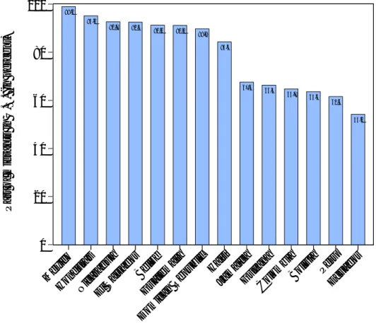
The recent years were marked by the increasing role of emigrants remit-tances in total international capital flows. In the aggregate, remitremit-tances are currently the second largest source of foreign exchange after foreign direct investment (Figure 1). For many developing countries, remittances represent a significant part of income (Figure 2).
Figure 1: Remittances, Foreign Direct investment and Official Development Assistance received in Developing countries.
19800 1982 1984 1986 1988 1990 1992 1994 1996 1998 2000 2002 2004 2006 50 100 150 200 250 300 350 400 450 500 550 Billions of US dollars Remittances
Foreign Direct Investment (FDI) Official Development Assistance (ODA)
Source: World Bank WDI.
The literature on the determinants of remittances is dominated by two approaches: one approach focusing on micro-economic aspects, and the other focusing on macro-economic factors. In the micro-economic approach, Lucas and Stark (1985) were the first to build a formal model for analyzing the motivations to remit. These authors point out that remittances are sent for many of reasons, ranging from pure altruism motives to pure self-interest mo-tives. According to Lucas and Stark (1985), migrant workers can be classified as altruistic if remittances increase with declines in family income at home, while self-interest motives would dominate if remittances were positively re-lated with home economic performances. Some empirical papers (Lucas and Stark, 1985; Ilahi and Jafarey, 1999; Agarwal and Horowitz, 2002, Adams, 2009, among others) have tried to test the altruistic hypothesis against the self-interest hypothesis using micro-economic variables.
At the same time, other researchers have used macroeconomic variables to analyze the macroeconomic factors that impact remittances. In order to
cap-Figure 2: Top remittances-recipient in 2008 (remittances as percent of GDP) 0 10 20 30 40 Tajikistan Tonga
Moldova Lesotho Guyana Lebanon Samoa Jordan Honduras
Kyrgyz Republic Jamaica
El Salvador Haiti Nepal
Bosnia and Herzegovina Nicaragua Guatemala
Serbia Philippines
Albania Cape Verde Bangladesh
Dominican Republic Armenia Togo 45.5 39.4 34.1 27.7 25.8 23.7 22.8 21.7 21.5 19.1 18.8 18.2 18.2 16.8 16.6 12.9 12.6 12.2 11.3 9.9 9.7 9.6 9.3 9.2 9.2 P e rc e n t o f G D P
Source: World Bank WDI.
ture host economic conditions, host country GDP (income) is generally used as explanatory variable, since this variable can reflect economic prosperity of migrant in host country. Elbadawi and Rocha (1992), El-Sakka and McNabb (1999)and Lianos (1997) found a significant positive effect of host income on remittances. Some previous papers also used host unemployment rate to proxy for host economic conditions. Higgins et al. (2004) showed evidence of a significant positive effect of host unemployment rate on remittances, while Lianos (1997) found an ambiguous impact of host unemployment rate on remittances.
To capture economic conditions in home country (altruistic motivation), generally, the variable employed is GDP in home country. The idea is that, if the altruistic motives dominates, the more depressed income in the home country is, the more remittances increase. On contrary, if the self-interest motives dominates, the more expanded income in the home country is (im-provement in home economic conditions), the more remittances increase. El-Sakka and McNabb (1999) and Lianos (1997) showed a non significant impact of home income on remittances, while Higgins et al. (2004) indicated
a positive relationship between home income and remittances. Higgins et al. (2004) also found that exchange rate uncertainty (a measure of risk in home country) is an important determinant of remittances.
To check for the assumption of self-interest motivations, some previous studies have also used variables designed to capture portfolio effects due to the difference in financial returns between home and host countries. There-fore, the difference between the domestic and foreign interest rates may be used to investigate self-interest motivations. The studies by Swamy (1981) and Elbadawi and Rocha (1992) did not find a significant effect of this dif-ference in interest rates, while El-Sakka and McNabb (1999) reported it with a negative and highly significant impact. Lianos (1997) considered the for-eign and domestic interest rates separately and found positive and significant impact for the domestic interest rate, but inconclusive result for the foreign interest rate under different formulations.
Sayan (2006) investigates the correlation between remittances and busi-ness cycles using data from 12 developing countries during 1976-2003. This study found that countercyclicality or procyclicality of remittances is not commonly observed across these countries.
The techniques used by the papers mentioned above to investigate the relationship between remittances and macroeconomic variables are generally a single-equation-based approach. To tackle the interaction problem between remittances and its potential determinants, Huang and Vargas-Silva (2006) employ a VAR context by investigating whether remittances respond to the macroeconomic factors of host or home country. There is a potential causal link between remittances and home economic conditions. On the one hand, for altruistic or self-interest motives, remittances respond to home economic conditions. On the other hand, remittances can influence home economic variables. Huang and Vargas-Silva (2006) use in their VAR system: net remittances sent from the U.S. (or remittances received in Mexico), vari-ables capturing the U.S. economic activity, varivari-ables capturing Mexico eco-nomic (or weighted average of variables capturing ecoeco-nomic activity in the five biggest recipients of remittances from the U.S - Mexico, Brazil, Colom-bia, El Salvador and Dominican Republic-, weights given by the share of received remittances). These authors found evidence that the host coun-try (the U.S.) economic conditions seem to be the most important factor explaining remittances.
Contrary to Huang and Vargas-Silva (2006), in order to examine the re-sponse of remittances to host and home country economic considerations, this paper employs the panel VAR method. The use of panel VAR techniques allows to benefit from both the advantages of VAR approach and panel tech-niques. As mentioned above, the VAR approach addresses the endogeneity
problem by allowing the endogenous interaction between the variables in the system. The panel techniques tackle the problem of data limitation by taking the data from various countries. Moreover, the asymptotic results are easier to derive from a panel data.
This study uses data for 14 Latin American and Caribbean countries (Be-lize, Bolivia, Colombia, Dominican Republic, Ecuador, El Salvador, Guatemala, Guyana, Haiti, Honduras, Jamaica, Mexico, Nicaragua and Peru). These 14 countries were selected in order to facilitate the choice of host country. In-deed, the United States (U.S.) is the major destination of migrant from these countries, then the U.S. is considered as the only host country.
The results from this paper suggest that the economic conditions in host country (the U.S.) seem to be more important in explaining the fluctuations in remittances received in the 14 Latin American and Caribbean countries. By including both host and home country macroeconomic variables in panel VAR system, remittances respond significantly to host macroeconomic vari-ables, while they do not respond to home GDP.
The remainder of the paper is organized as follows. Section 2 presents a simple theoretical model that presents the potential macroeconomic de-terminants of remittances. Section 3 describes the data used in the econo-metric estimation. Section 4 presents the econoecono-metric methodology. Section 5 presents the empirical results and the interpretations of these empirical results. Finally, Section 6 concludes.
2
Theoretical framework
This section presents a simple two-period model that describes the behavior of a representative migrant born in home country and working in host coun-try. The model presented here has the same basic implications of most other
remittance models.1
In the first period, the migrant is assumed to maximize her or his utility by allocating her or his income between transfers to her or his family in the home country, her or his own consumption in the host country and saving. The migrant has the possibility to acquire financial/non-financial assets in both countries. These assets are assumed to yield a certain rate of return. In the second period, the agent consumes the saving made in the first period. Formally, the utility of migrant is given by:
Um(C1m, C2m, Cf) = u(C1m) + βu(C2m) + γu(Cf) (1)
1
where u′(C) > 0 and u′′(C) < 0 for C ∈ {Cm
1 , C2m, Cf} β ∈ (0, 1] is the
migrant’s time discount rate, γ ∈ (0, 1] is the degree of altruism towards the
family, Cm
t is migrant’s consumption at time t (t = 1, 2), Cf denotes the
migrant’s family’s consumption at home.
The resource constraints of migrants is given by the following equations:
C1m+ X + I = Ym (2)
C2m = (1 + r)I (3)
where X is the amount that migrant sends to sustain consumption of the
family at home, I represents the amount invested of current income Ym that
migrant earns in host country and r denotes the overall portfolio return.2
The consumption of migrant’s family Cf depends on the income earned
by migrant’s family at home, Yf, and the remittances received from migrant,
X. For simplicity, the consumption of migrant’s family is additively separable
in Yf and X. Formally,
Cf = Yf + X (4)
The migrant’s maximization program can be decomposed in two steps. In the first step, given her income in the host country, the migrant decides how much to allocate to consumption, savings and transfers to the family. Second, given total savings, the migrant solves a portfolio allocation prob-lem, by deciding how much to invest in the home and host countries.
The first step of the representative migrant’s problem is to maximize her or his utility subject to the constraints (2)and (3), in order to decides how much to allocate to consumption, savings and transfers to the family:
Max {Cm 1 ,C m 2 ,I,X} u(Cm 1 ) + βu(C2m) + γu(Yf + X) subject to C1m+ X + I = Ym and Cm 2 = (1 + r)I
This optimization problem can be formulated via the following Lagrangian:
L = u(Cm
1 ) + βu(C2m) + γu(Yf+ X) + λ(Ym− C1m− X − I) + µ((1 + r)I − C2m)
(5) The optimal solution of the program is given by the following equations:
2
u′(Cm 1 ) = λ (6) βu′(Cm 2 ) = µ (7) λ = µ(1 + r) (8) γu′(Cf) = λ (9)
Equations (6) -(9) are the first order conditions relatively to Cm
1 , C2m, I
and X, respectively.
Combining equations (7) and (8) yields
β(1 + r)u′(C2m) = λ (10)
Since u′′(Cf) < 0 and Cf = Yf+X, equation (9) shows that the more the
degree of altruism is strong (large γ ), the more remittances sent to sustain consumption, X, are large.
Using equations (6) and (10), the derivative of optimal level of remittances
sent to sustain consumption in home country X∗ with respect to Ym and Yf
are given by the following equations:
∂X∗ ∂Ym = β(1 + r)2u′′(Cm 1 )u′′(C2m) D > 0 (11) ∂X∗ ∂Yf = γu′′(Cf)[u′′(Cm 1 ) + β(1 + r)2u′′(C2m)] D < 0 (12)
where D = γu′′(Cf)[u′′(Cm
1 )+β(1+r)2u′′(C2m)]+β(1+r)2u′′(C1m)u′′(C2m) >
0
Equation (11) shows that the optimal level of transfer to sustain
consump-tion of family at home, X∗, is an increasing function of the income of migrant
in host country, Ym, i.e. migrant sends more money to sustain consumption
at home if his economic conditions improve. On the contrary, equation (12) shows that the optimal level of transfer to sustain consumption is a decreas-ing function of the income of family at home, i.e migrant sends more money to sustain consumption at home if home economic conditions deteriorate.
The second step of the optimization problem is the portfolio allocation.
In this step, given the optimal investment amount I∗ and the exogenous
return on assets in both countries rhost and rhome, the migrant chooses the
asset mix Ihost and Ihome that maximizes the return of the portfolio. This
Max
{Ihost
,Ihome
}[r host
Ihost+ rhomeIhome]
subject to Ihost+ Ihome= I
The optimal choices of Ihost and Ihome are given as follows:
Ihost∗ = 0 and Ihome∗= I∗ if rhost < rhome
Ihost∗ = I∗ and Ihome∗ = 0 if rhost > rhome
Ihost∗ ∈ [0, I∗] and Ihome∗ = I∗− Ihost∗ if rhost = rhome
(13)
Condition (13) shows that self-interested remittances, Ihome, is positively
(negatively) determined by the return on assets in home (host) country. Thus, self-interest remittances are positively related to improvements in the economic conditions of home country: in response to an improvement in the economic conditions of home country, migrant sends more money in order to exploit investment opportunities in the home country.
The total amount of worker’s remittances, REM , is the sum of altruistic
remittances, X∗, and self-interest remittances, Ihome∗ (remittances sent in
order to exploit investment opportunities in home country): REM = X∗+
Ihome∗.
The results of this theoretical model, in a macroeconomic framework, can be summarized as follows. Since an increase in migrant income allows migrant to send more money for altruistic motives and to make more in-vestment that can take place in host or home country, an improvement in the economic conditions of the host country has a positive effect on the to-tal remittances (altruistic remittances plus self-interest remittances). While the relationship between total remittances and the conditions in the home country is ambiguous. If the altruistic motive dominates, a negative rela-tionship is to be expected. However, since improvement in home economic conditions will reflect an increase in expected return on assets, if the motive for remitting is to exploit investment opportunities, remittances will respond positively to improvement in the economic conditions of the home country.
This model allows to hypothesize how the total remittances respond to changes in the economic conditions of host and home countries. The empirical section of this paper estimates those responses.
3
Data
Annual data over the period 1990-2007 from 14 Latin American and Caribbean countries (Belize, Bolivia, Colombia, Dominican Republic, Ecuador, El Sal-vador, Guatemala, Guyana, Haiti, Honduras, Jamaica, Mexico, Nicaragua
and Peru) where remittances represent a significant part of income (Figure 3) are used. These 14 countries are selected in order to facilitate the choice of host country. Indeed, the United States (U.S.) is the major destination of migrant from these countries, thus the U.S. is the only host country consid-ered (Figure 4). Figure 4 shows that the U.S. receives more than 90 percent of migrants from Mexico, Honduras, Nicaragua, El Salvador and Belize, more than 80 percent of migrants from Guatemala and Dominican Republic, more than 60 percent of migrants from Jamaica, Guyana, Colombia, Bolivia and Peru, and 54.2 percent of migrants from Ecuador. So, the U.S. macroeco-nomic variables are used to capture ecomacroeco-nomic conditions in host country. The U.S variables used are: U.S. real GDP per capita , U.S. Federal Fund Rate (U.S. FFR). The U.S. real GDP is used to measure the income in host country. The U.S. Federal Fund rate (U.S. FFR) is used to reflect expected
future changes in U.S. economy.3 An increase in the U.S. FFR can impact
remittances through two channels. First, it should have a negative effect on the economic conditions of host country which leads to a fall in remittances. Second, it has a positive effect on return on asset of the U.S and this has a negative effect on self-interest remittances.
To capture the economic conditions of home country, real GDP per capita of home country (Home GDP) is used. Real GDP of home country is used to capture improvement in economic conditions of the home country. As mentioned above, the predicted effect of this variable in a model of remit-tances depends on what are the motives of immigrant workers to remit. If they are altruistic, in presence of downturns in the home economy, migrant would send more money to sustain family members. On the other hand, if immigrant workers are self-interested, remittances will respond positively to an improvement in the economic conditions of the home country.
Table 1 reports the results of the unit root tests for the variables. Since host variables (U.S. GDP and U.S. FFR) are the same for all the countries in the panel, a standard Augmented Dickey Fuller (ADF) test is employed. For remittances (REM) and home GDP, the panel unit root test of Im, Pesaran and Shin (2003) (IPS) is employed. The results of the unit root tests show that all the variables are I(1).
Table 2 reports the results of the seven cointegration tests (panel v test, panel rho test,panel non parametric test, panel parametric test, group mean rho test, group mean non parametric test and group mean parametric test) proposed by Pedroni (1999, 2004). These tests are based on the null hypoth-esis of no cointegration, and heterogeneity is allowed under the alternative
3
According to Bernanke and Blinder (1992), the U.S. Federal Fund Rate is the best measure of the U.S. monetary policy.
Figure 3: Remittances Inflows in Latin American and Caribbean countries, 2007 (percent of GDP). 0 4 8 12 16 20 24 28 Guyana
HondurasJamaicaEl Salvador Haiti
NicaraguaGuatemala Dominican Republic
BoliviaEcuadorBelizeMexico Colombia Peru 25.8 21.5 18.8 18.2 18.2 12.9 12.6 9.3 7.1 7.0 5.9 2.7 2.2 2.0 Source: WDI.
hypothesis. The null hypothesis of no cointegration cannot be rejected by these tests. Particularly, the group mean parametric t-test and panel v test significantly accept the null hypothesis of no cointegration. Simulations made by Pedroni (2004) show that, in small samples (T ≈ 20), the group mean parametric t-test is more powerful than the other tests, followed by the panel v test. As a result, the empirical properties of the variables indicate that es-timating the VAR in first differences without imposing any cointegration relationships is more appropriate.
Table 1: Unit root test
Variables ADF test IPS test
ln(U.S.GDP ) -1.9007 (0.6126) ∆ln(U.S.GDP ) -2.5127 (0.0155) U.S.F F R -2.7756 (0.0826) ∆U.S.F F R -2.5127 (0.0155) ln(REM ) 0.6223 (0.7331) ∆ln(REM ) 7.9113 (0.0000) ln(HomeGDP ) 3.0703 (0.9989) ∆ln(HomeGDP ) -6.8505 (0.0000)
Notes: P-values are given in parentheses.
Table 2: Panel cointegration tests Within-dimension
Statistic p-value
Panel v test -1.0084 0.2399
Panel rho test 2.6187 0.1129
Panel non parametric test 1.9190 0.0633
Panel parametric test 1.0734 0.0734
Between-dimension
t-stat p-value
Group rho test 4.1120* 0.1001
Group non parametric test 2.1241* 0.1418
Group parametric test 1.0593 0.2276
Figure 4: Part of migrants in U.S. 0 20 40 60 80 100 Mexico HondurasNicaragua El Salvador Belize Guatemala Domican Republic Haiti
JamaicaGuyanaColombiaBolivia Peru Ecuador 99.0 95.1 92.7 92.5 91.2 91.1 89.8 84.3 67.6 66.3 64.7 63.6 61.6 54.2 Pa rt o f mi g ra n ts in U .S. (i n p e rce n t)
Source: Database on Immigrants and Expatriates (OECD).
4
Econometric methodology
The impulse response functions (IRFs) and variance decompositions (VDC) are computed from the panel VAR. As mentioned above, the panel VAR approach allows to benefit both for the advantages of VAR approach and panel techniques. The VAR approach addresses the endogeneity problem by allowing endogenous interactions between the variables in the system. The panel techniques tackle the problem of data limitation by taking the data from various countries and the asymptotic results are easier to derive for panel data.
The initial econometric model takes the following reduced form:
Yitis a vector of stationary variables including: ∆ln(U.S. GDP ), ∆U.S. F F R,
∆ln(REM ) and ∆ln(Home GDP ). Γ(L) is a matrix polynomial in the lag
operator with Γ(L) = Γ1L1 + Γ2L2 + . . . + ΓpLp, ui is the country specific
effect and ǫit is idiosyncratic error.
An issue in estimating this model concerns the presence of fixed effects. Since fixed effects are correlated with the regressors due to lags of the depen-dent variable, following Love and Zicchino (2006), forward mean differencing (the Helmert procedure) is used in order to remove the fixed effects. In this procedure, all variables in the model are transformed to deviations from
for-ward means. Let ¯ym
it =
PTi
s=t+1ymis/(Ti − t) denotes the means constructed
from the future values of ym
it a variable in the vector Yit = (y1it, y2it, . . . , yitM)′,
where Ti denotes the last period of data available for a given country series
. Let ¯ǫm
it denotes the same thing of ǫmit, where ǫit = (ǫ1it, ǫ2it, . . . , ǫMit)′. The
transformations are given by: ˜ ym it = δit(ymit − ¯yit) (15) and ˜ǫmit = δit(ǫmit − ¯ǫ m it) (16)
where δit = p(Ti− t)/(Ti− t + 1). For the last year of data, this
trans-formation cannot be calculated, since there are no future value for the con-struction of the forward means. The final transformed model is thus given by:
˜
Yit= Γ(L) ˜Yit+ ˜ǫit (17)
where ˜Yit = (˜yit1, ˜yit2, . . . , ˜yMit)′ and ˜ǫit= (˜ǫ1it, ˜ǫ2it, . . . , ˜ǫMit )′
This transformation is an orthogonal deviation, in which each observation is expressed as a deviation of average future observations. Each observation is weighed to standardize the variance. If the original errors are not autocor-related and have a constant variance, the transformed errors should exhibit similar properties. Thus, this transformation preserves homoscedasticity and does not induce serial correlation (Arellano and Bover, 1995). The lagged val-ues of regressors are used as instruments to estimate the transformed model by the generalized method of moments (GMM).
After estimating the parameters of the panel VAR, the impulse response functions (IRFs) and the variance decomposition (VDC) are computed using
the Cholesky decomposition.4 The assumption behind the Cholesky
decom-position is that series listed first in the VAR order impact the other variables contemporaneously, while series listed later in the VAR order impact those listed first only with lag. Therefore, variables listed first in the VAR order are considered to be more exogenous. The U.S. GDP is placed first in the ordering, followed by the U.S. FFR. This ordering structure implies that innovations in the U.S. GDP can contemporaneously influence the imple-mentation of monetary policy by the Federal Reserve. While, changes in the U.S. FFR will impact the U.S. GDP only with a lag. Remittances is placed after the U.S. variables and home GDP is placed last in the ordering. Then remittances are assumed to contemporaneously impact home GDP, while re-mittances respond to home GDP only with a lag. The robustness analysis shows that changing this ordering does not significantly impact the results.
5
Empirical results
his section presents the impulse response functions and the variance decom-position from the panel VAR. The correct lag length selection is essential for a VAR model: too short lags fail to capture all the system’s dynamics, resulting from omitted variable bias; while too many lags suffer from a loss of degrees of freedom, because of over-parametrization. The Akaike Infor-mation Criterion (AIC) and the Schwarz Bayesian Criterion (SBS) indicate more than three lags as the appropriate lags for most countries. Two lags and three lags are better than one lag, and three lags are better than two lags. Greater lags than three are not possible due to a nearly singular matrix of determinants. Using the maximal lag as possible two lags are chosen. Then, the estimated panel VAR is the following:
∆ln(U.S.GDP ) ∆U.S.F F R ∆ln(REM ) ∆ln(HomeGDP ) = Γ1 ∆ln(U.S.GDP )(−1) ∆U.S.F F R(−1) ∆ln(REM )(−1) ∆ln(HomeGDP )(−1) + Γ2 ∆ln(U.S.GDP )(−2) ∆U.S.F F R(−2) ∆ln(REM )(−2) ∆ln(HomeGDP )(−2) + ǫ1 ǫ2 ǫ3 ǫ4
The estimate results of the 4-variable panel VAR(2) are given in Table 3. The IRFs are displayed in Figures 5 and 6. The VDC results are reported in Tables 4 and 5
Figure 5 shows that remittances positively respond to a shock on U.S. GDP, but negatively respond to a shock on U.S. FFR. The response of remit-tances to U.S. GDP is significant until at least seven years, and the response
4
The panel VAR is estimated by using the package provided by Inessa Love. This package is a Stata programs for Love (2001) and it is used in Love and Zicchino (2006).
Table 3: Estimate results of 4-variable panel VAR(2) model
Dependent variables
∆ln(U.S.GDP ) ∆U.S.F F R ∆ln(REM ) ∆ln(HomeGDP ) ∆ln(U.S.GDP )(−1) 0.862 (8.07)*** 0.695(8.07)*** 5.821(1.95)** 0.325(1.17) ∆ln(U.S.GDP )(−2) 0.278(3.56)*** -0.157(-1.06) 8.148(2.46)** 0.813(1.99)** ∆U.S.F F R(−1) -0.632(-4.94)*** 0.315(3.95)*** -6.999(-2.14)** 0.470(1.34) ∆U.S.F F R(−2) -0.089(-1.84)* -0.141(-1.66)* -0.757(-0.39) 0.356(2.18)** ∆ln(REM )(−1) 0.004(1.46) -0.001(-0.509) 0.128(1.988)** 0.014(2.51)** ∆ln(REM )(−2) 0.002(0.86) 0.000(0.64) -0.028(-0.51 -0.004(-0.63)) ∆ln(HomeGDP )(−1) (0.080)(2.21)** 0.033(1.05) 1.709(1.64)** 0.231(2.69)*** ∆ln(HomeGDP )(−2) 0.034(0.90) 0.021(0.635) 0.728(0.69) 0.016(0.18) N obs 217
The 4-variable panel VAR (2) model is estimated by GMM, country fixed effects are removed prior to estimation (by forward mean differencing). Reported numbers show the coefficients of regressing the column variables on lags of the row variables. Het-eroskedasticity adjusted t-statistics are in parentheses. *,**,***, indicate significance at 10%, 5% and 1% level, respectively.
of remittances to U.S. FFR is significant until four periods. The response of remittances to a shock on home GDP is insignificant. The variance decompo-sition results in Table 4 confirms these findings. The results in Table 4 show that U.S. GDP and U.S. FFR explain about 26 and 7% of the fluctuations in remittances after 10 years, respectively. While home GDP explains only 4% of of the fluctuations in remittances after ten years.
For robust analysis, the IRFs and the VDC are re-evaluated by changing the ordering in the VAR. In this new ordering, home GDP is placed before remittances, thus remittances is the last variable in the system. For this new ordering, the impulse response functions are displayed in Figure 6 and the variance decomposition results are reported in Table 5. The results from this new ordering are not significantly different to those before.
The results can be interpreted as follow. An increase in U.S GDP reflect-ing an improvement of migrant economic situation leads to an increase in re-mittances send from the U.S. An increase in U.S. FFR reflecting a monetary contraction leads to a decrease U.S. output and to a decrease in remittances sent from the U.S. The fact that remittances do not respond to home income can be interpreted as the combining of altruistic and self-interested motives leading to a mitigated effect.
To sum up, host economic conditions are an important factor driving re-mittance cycles while home economic conditions do not have a significant in-fluence on remittances. This result is line with previews studies using macroe-conomic variables (El-Sakka and McNabb, 1999; Lianos, 1997; and, Huang and Vargas-Silva, 2006). As mentioned above, El-Sakka and McNabb (1999)
Figure 5: Impulse responses of remittances 0 1 2 3 4 5 6 −0.05 0 0.05 0.1 0.15 Response of remittances to US GDP time 0 1 2 3 4 5 6 −0.1 −0.05 0 0.05 0.1 Response of remittances to US FFR time 0 1 2 3 4 5 6 −0.05 0 0.05 0.1 0.15
Response of remittances to Home GDP
time
Notes: Estimated regressions use two lags of each variable. The Cholesky decomposition ordering is: ∆ln(U.S. GDP ), ∆U.S. F F R, ∆ln(REM ), ∆ln(Home GDP ). The solid line shows the response of remittances to a shock on variables in the system. The dashed lines indicate five standard confidence band around the estimate. Error are generated by Monte-Carlo with 500 repetitions
and Lianos (1997) found a positive impact of host GDP on remittances, but no significant impact of home GDP. Particularly, the findings from this pa-per are very related to the results from the vector autoregressive analysis by Huang and Vargas-Silva, 2006. Using average data on Brazil, Colombia, the Dominican Republic, El Salvador, Mexico, Huang and Vargas-Silva, 2006 found that that remittances respond more to changes in the macroeconomic conditions of the U.S., than to changes in the macroeconomic conditions of the home country. The results from this paper are also in line with the re-sults in Sayan (2006). The paper by Sayan (2006) examines the link between remittances and business cycles of 12 developing countries over the period 1976-203. The results from this study suggest evidence that the cyclicality
Figure 6: Impulse responses of remittances (changing in VAR ordering) 0 1 2 3 4 5 6 −0.05 0 0.05 0.1 0.15 Response of remittances to US GDP time 0 1 2 3 4 5 6 −0.1 −0.05 0 0.05 0.1 Response of remittances to US FFR time 0 1 2 3 4 5 6 −0.05 0 0.05 0.1 0.15
Response of remittances to Home GDP
time
Notes: Estimated regressions use two lags of each variable. The Cholesky decomposition ordering is: ∆ln(U.S. GDP ), ∆U.S. F F R, ∆ln(REM ), ∆ln(Home GDP ). The solid line shows the response of remittances to a shock on variables in the system. The dashed lines indicate five standard confidence band around the estimate. Error are generated by Monte-Carlo with 500 repetitions
property of remittances depends on country under consideration.
These results suggest some important policy implications. First, since re-mittances seem to not respond to home economy conditions, if rere-mittances- remittances-receiving countries want to receive more remittances they should consider in-dividual and demographic variables (Huang and Vargas-Silva, 2006). Second, in their planning for future growth of remittances, labor-exporting countries should explicitly account for future economic prospects of the major desti-nation countries of their emigrants.
Table 4: Variance decomposition of remittances in Model 1 Percentage of the variation in remittances explained by
Horizon U.S. GDP U.S. FFR Home GDP
2 13.49 0.1 0.02
5 17.08 7.11 3.37
10 25.66 7.10 4.07
Notes: estimated regressions use two lags of each variable. The Cholesky decomposition ordering is: ∆ln(U.S. GDP ) ∆U.S. F F R, ∆ln(REM ), ∆ln(Home GDP ).
Table 5: Variance decomposition of remittances in Model 2 Percentage of the variation in remittances explained by
Horizon U.S. GDP U.S. FFR Home GDP
2 13.49 1.27 2.17
5 16.27 5.74 3.67
10 25.66 7.10 4.32
Notes: estimated regressions use three lags of each variable. The Cholesky decomposition ordering is: ∆ln(U.S. GDP ) ∆U.S. F F R, ∆ln(Home GDP ), ∆ln(REM ).
6
Conclusion
This paper examines whether the host or the home country’s economic con-ditions influence remittances flows. To conduct this empirical study, a panel VAR approach is employed in order to benefit from both the advantages of VAR approach and panel techniques. Annual data over the period 1990-2007 from 14 Latin American and Caribbean countries (Belize, Bolivia, Colom-bia, Dominican Republic, Ecuador, El Salvador, Guatemala, Guyana, Haiti, Honduras, Jamaica, Mexico, Nicaragua and Peru). These 14 countries were selected in order to consider the U.S. as the only host country, since the U.S. is the major destination of migrant from these countries. The results from this paper show evidence that host economic conditions seem to be an important factor driving remittances cycles, while home economic conditions do not have a significant influence remittances.
These results have some important policy implications. First, since remit-tances do not respond to home economic conditions, if recipients countries want to receive more remittances, they should pay attention to individual and demographic variables rather than home macroeconomic variables (Huang and Vargas-Silva, 2006). Second, in their planning for future growth of re-mittances, remittances recipient countries should explicitly take into account
future economic prospects in the major destination countries of their emi-grants. In other words, receiving countries should figure out that remittances is another channel through which host economy shocks transmit. This is par-ticularly relevant for countries that receive a high amount of remittances.
Since remittances are explained by exogenous factors that are indepen-dent of home business cycles, and, since remittances can impact home econ-omy, remittance shocks can be considered as a source of fluctuations of home economy. This should be the goal of the future research.
Appendix
A.1
Countries included in the sample
These fourteen home countries are: Belize, Bolivia, Colombia, Dominican Republic, Ecuador, El Salvador, Guatemala, Guyana, Haiti, Honduras, Ja-maica, Mexico, Nicaragua and Peru. The United States is the only host country.
A.2
Variables and their sources
This appendix provides the definition and data sources for the variables used in the regressions that are reported in this paper.
• Remittances: Sum of worker’s remittances, migrant transfers in real terms (constant 2000 US$). The data source is World Development Indicator (World bank).
• Home GDP: Real GDP per capita (constant 2000 US$) of home coun-try. The data source is World Development Indicator (World Bank). • U.S (Host) GDP:Real GDP per capita (constant 2000 US$) of United
States. The data source is World Development Indicator (World Bank). • U.S. FFR: U.S. Federal Funds Rate. The data source is International
References
Agarwal, R., and Horowitz, A. W. (2002). Are international remittances al-truism or insurance: Evidence from Guyana using multiple-migrant house-holds. World Development 30, 2033-2044.
Adams, R. H. (2009). The Determinants of international remittances in de-veloping countries. World Development 37, 93-103.
Arrelano, M., and Bover, O. (1995). Another look at the instrumental vari-able estimation of error-components model. Journal of Econometrics 68, 29-51.
Bernanke, B., and Blinder, A. (1992). The Federal funds rate and the chan-nels of monetary transmission. American Economic Review 82, 901-921. Elbadawi, I., and Rocha, R. R. (1992). Determinants of expatriate workers’
remittances in North Africa and Europe. The World Bank Working Papers 1038, 1-56.
El-Sakka, M.I.T, andMcNabb, R. (1999). The Macroeconomic determinants of emigrant remittances. World Development 27, 1493-1502.
Higgins, M. L., Hysenbegasi, A., and Pozo, S. (2004). Exchange-rate uncer-taintyand workers’ remittances. Applied Financial Economics 14, 403-411. Huang P., and Vargas-Silva C. (2006). Macroeconomic determinants of work-ers’ remittances: Host vs. home country’s economic conditions. Journal of
International Trade and Economic Development 15, 81-99.
Ilahi, N., Jafarey, S. (1999). Guestworker migration, remittances and the extended family: Evidence from Pakistan. Journal of Development
Eco-nomics 58, 485-512.
Im, K., Pesaran, M. H., and Shin, Y. (2003). Testing for unit roots in het-erogenous panel. Journal of Econometrics 115, 53-74.
Lianos, T.P. (1997). Factors determining migrant remittances: The case of Greece. International Migration Review 31, 72-87.
Love, I. (2001). Estimating panel-data autoregressions, package of programs for Stata. Columbia University, Mimeo.
Love, I., and Zicchino, L. (2006). Financial development and dynamic in-vestment behavior: Evidence from a panel VAR. The Quarterly Review of
Economics and Finance 46, 190-210.
Lucas, R.E.B, and Stark, O. (1985). Motivations to remit: Evidence from Botswana. Journal of Political Economy 93, 901-918.
Pedroni, P., 1999. Critical values for cointegration tests in heterogeneous pan-els with multiple regressors. Oxford Bulletin for Economics and Statistics
61, 653-670.
———– (2004). Panel cointegration: asymptotic and finite sample prop-erties of pooled time series with an application to the PPP hypothesis.
Econometic Theory 20, 597-625.
Rapoport, H. and Docquier, F. (2005). The economics of migrants’ remit-tances. In L.,A, Gerard-Varet, S-C Kolm and J. Mercier (Eds) Handbook
of the Economics of Reciprocity, Giving and Altruism, Amsterdam: North
Holland.
Sayan, S. (2006). Business cycles and workers’ remittances: How do migrant workers respond to cyclical ovements of GDP at home? IMF Working Paper 06/52.
Stark, O. (1995). Altruism and Beyond. Oxford and Cambridge : Basil Black-well.
Stark, O., Taylor, J., E., and Yitzhaki, S. (1986). Remittances and inequality.
The Economic Journal 96, 722-740.
Swamy, G., 1981. International migrant workers’ remittances: Issues and prospects. World Bank, Staff Working Paper 481.