HAL Id: hal-02378197
https://hal.archives-ouvertes.fr/hal-02378197v2
Submitted on 29 Nov 2019
HAL is a multi-disciplinary open access
archive for the deposit and dissemination of
sci-entific research documents, whether they are
pub-lished or not. The documents may come from
teaching and research institutions in France or
L’archive ouverte pluridisciplinaire HAL, est
destinée au dépôt et à la diffusion de documents
scientifiques de niveau recherche, publiés ou non,
émanant des établissements d’enseignement et de
recherche français ou étrangers, des laboratoires
A Differential Algebra Introduction For Tropical
Differential Geometry
François Boulier
To cite this version:
François Boulier. A Differential Algebra Introduction For Tropical Differential Geometry. Doctoral.
United Kingdom. 2019. �hal-02378197v2�
A Differential Algebra Introduction For Tropical Differential
Geometry
François Boulier
∗†November 29, 2019
These notes correspond to an introductory course to the workshop on tropical differential geometry, organized in December 2019 at the Queen Mary College of the University of London.
I would like to thank many colleagues for their feedback. In particular, François Lemaire, Adrien Poteaux, Julien Sebag, David Bourqui and Mercedes Haiech.
Contents
1 Formal Power Series Solutions of Differential Ideals 2
1.1 Differential Rings . . . 2
1.2 Differential Polynomials . . . 3
1.2.1 An Example . . . 3
1.3 Differential Ideals . . . 4
1.4 Formal Power Series (Ordinary Case) . . . 5
1.4.1 Informal Introduction . . . 5
1.4.2 On the Expansion Point . . . 6
1.4.3 Summary . . . 7
1.5 Formal Power Series (Partial Case) . . . 7
1.6 Denef and Lipshitz Undecidability Result . . . 9
1.7 General Formulas . . . 11
2 A Differential Theorem of Zeros 11 2.1 Characteristic Sets — The Nonconstructive Definition . . . 11
2.2 Ritt’s Reduction Algorithms . . . 14
2.3 Characteristic Sets of Prime Differential Ideals . . . 15
2.4 The Ritt-Raudenbush Basis Theorem . . . 16
2.5 Zeros of a Prime Differential Ideal . . . 19
2.6 A Differential Theorem of Zeros . . . 21
3 Differential Elimination Methods 22 3.1 Characteristic Sets — The Constructive Definition . . . 22
3.1.1 The Nondifferential Obstacle . . . 22
3.1.2 The Differential Obstacle . . . 24
3.2 Identifying Zero Divisors . . . 25
3.2.1 Decision Algorithms Available With Regular Chains . . . 26
3.2.2 Testing the Inclusion of Differential Ideals . . . 27
∗Univ. Lille, CNRS, Centrale Lille, Inria, UMR 9189 - CRIStAL - Centre de Recherche en Informatique Signal et Automatique
de Lille, F-59000 Lille, France.
3.3 Normal Forms and Formal Power Series Solutions . . . 28
3.3.1 Computation of Normal Forms . . . 28
3.3.2 Application to the Computation of Formal Power Series Solutions . . . 29
3.4 A Sketched Elimination Algorithm . . . 31
3.4.1 An Ordinary Differential Example . . . 31
3.4.2 A Partial Differential Example . . . 33
1 Formal Power Series Solutions of Differential Ideals
Twenty years ago I had the opportunity to teach differential elimination methods at Paris VI University (today Sorbonne University) in some Master course. The beginning of the course — up to differential ideals — is taught quite easily. But difficulties actually occur as soon as one writes a first equation: what do you mean by a solution of a differential equation whose left hand side is a general differential polynomial ? The approach followed by Ritt (a solution is a prime differential ideal which contains the equation) is very elegant but it is also terribly abstract for students. This time, I have decided to start with a more tedious but much more intuitive approach: we look for formal power series solutions. This approach actually perfectly suits the general context of the workshop.
The main issue of this section is: what about expansion points of formal power series ? They actually play an important role since the problem of the existence of formal power series solution of differential ideal is algorithmically decidable if the expansion point is unspecified while it is undecidable if it is fixed. The undecidability result is given in this section.
1.1
Differential Rings
Reference books are [17] and [12]. The following basic notions are introduced in [12, chap. I, 1].
An operator δ on a ring is called a derivation operator if δ(a + b) = δa + δb and δ(a b) = (δa) b + a δb for all elements a, b of the ring.
A differential ringR is defined as a ring with finitely many derivation operators which commute pairwise
i.e. such that δ1δ2a = δ2δ1a for all derivation operators δ1, δ2and all a∈ R.
A differential field is a differential ring which is a field. If the number m of derivation operators is equal to 1 then the differential ring is said to be ordinary. If it is greater than 1, the differential ring is said to be
partial.
The operator δ which maps every element of a ring to zero is a derivation so that every ring can be viewed as a trivial differential ring. If the ring is the field Q of the rational numbers, this derivation is the only possible one since
δ(0) = δ(0 + 0) = 2 δ(0) = 0 ,
δ(1) = δ(1× 1) = 2 δ(1) = 0 ,
hence the derivative of any rational number must be zero. More generally, it can be proved that the derivative of any complex number must be zero.
The equations we handle will have coefficients in some differential fieldF such that Q ⊂ F ⊂ C. Since a constant is any element whose derivative is zero, we see thatF is a field of constants and has characteristic
zero.
In the context of tropical differential geometry, it may be useful to introduce “independent variables”. We will see later how to handle them formally in differential algebra. For the moment, let us just say that the symbols x1, . . . , xm are supposed to be related to the derivation operators δ1, . . . , δm by the relations: δixi= 1 and δixj= 0 for all 1≤ i, j ≤ m such that i ̸= j. Thus we may interpret δias the partial derivative ∂/∂xi. In the ordinary context, the derivation operator can thus be interpreted as d/dx. However let us
stress that Ritt’s theory and an important part of Kolchin’s one do not require these assumptions and deal with an abstract differential fieldF of characteristic zero.
1.2
Differential Polynomials
From the differential algebra point of view, differential indeterminates are symbols such as u, v over which derivation operators may apply, giving an infinite set of derivatives. In the ordinary case, interpreting δ as d/dx, one may view differential indeterminates as representing unknown functions u(x) and v(x) and their derivatives
u, v, ˙u, ˙v, ¨u, ¨v, . . . , u(r), v(r), . . .
as representing the functions obtained by differentiation.
In the partial case, interpreting the derivation operators as δi = ∂/∂xi for 1 ≤ i ≤ m, one may view
differential indeterminates as representing unknown functions u(x1, . . . , xm) and v(x1, . . . , xm) and their
derivatives as representing the functions obtained by partial differentiations.
In the general case it is convenient, following [12, chap. I, 1] to introduce the commutative semigroup (written multiplicatively) Θ generated by the derivation operators. Each derivative operator θ∈ Θ has the
form
θ = δe1 1 · · · δ
em m
where e1, . . . , em ∈ N (the set of the nonnegative integers). Then the corresponding derivative of the
differential indeterminate (say) u will be denoted
θu or uxe1
1 ···xemm .
It represents the function
∂e1+···+emu ∂xe1 1 · · · ∂x em m (x1, . . . , xm) .
The nonnegative integer e1+· · · + em is said to be the order of the derivative operator θ. A derivative
operator θ is said to be proper if its order is strictly positive.
If F is a differential field and U = {u1, . . . , un} is a set of n differential indeterminates then the
poly-nomials in the derivatives in ΘU , with coefficients inF — the elements of F [ΘU] — are called differential polynomials. All together, they form a differential polynomial ring denoted
F {u1, . . . , un} .
1.2.1 An Example
Let us consider the ordinary differential polynomial ringF {u}. Here is an example of a differential
polyno-mial p∈ F {u} and its first derivatives:
p = u˙2+ u3,
˙
p = 2 ˙u ¨u + 3 u2u ,˙ ¨
p = 2 ˙u u(3)+ 2 ¨u2+ 3 u2u + 6 u ˙¨ u2.
In the sequel, we will define leading derivatives through the general concept of rankings. For the moment, let us just claim that ˙u, ¨u, u(3) are the leading derivatives of p, ˙p, ¨p. Observe that: 1) each proper derivative
of p has degree 1 in its leading derivative; and 2) these leading derivatives all have the same polynomial as coefficient. It is the so-called separant of p i.e. the partial derivative of the differential polynomial p w.r.t. its leading derivative
separant of p = ∂p
1.3
Differential Ideals
LetR denote the differential polynomial ring F {u1, . . . , un} with m > 0 derivation operators. The following
definitions are borrowed from [17, chap. I, 7] in the ordinary case. They readily apply to the general case, as pointed out in [17, chap. IX].
A nonempty subset A of R is said to be a differential ideal of R if:
1. it is an ideal ofR and
2. it is stable under the action of the derivations i.e. if it is such that p∈ A ⇒ θp ∈ A for all derivation
operator θ∈ Θ.
A differential ideal contains an infinite number of differential polynomials unless it consists of the single differential polynomial 0. The intersection of any finite or infinite number of differential ideals is a differential ideal.
A differential ideal A is said to be perfect if it is equal to its radical i.e. if (∃d ∈ N, pd ∈ A) ⇒ p ∈ A.
The intersection of any finite or infinite number of perfect differential ideals is a perfect differential ideal. A differential ideal A is said to be prime if it is prime in the usual sense i.e. if p q∈ A ⇒ (p ∈ A or q ∈ A). Every prime differential ideal is perfect.
Let Σ be any subset ofR.
One denotes [Σ] the differential ideal ofR generated by Σ. It is defined as the intersection of all differential
ideals of R containing Σ. It is the set of all finite linear combinations, with arbitrary elements of R for
coefficients, of elements of Σ and their derivatives of any order.
One denotes {Σ} the perfect differential ideal of R generated by Σ. It is defined as the intersection of all
perfect differential ideals ofR containing Σ.
It is clear that [Σ]⊂ {Σ}. More precisely, we have the following
Proposition 1 Let Σ be any subset ofR. Then {Σ} =√[Σ]. With words,{Σ} is the set of all differential
polynomials p∈ R for which there exists some r ∈ N such that pr∈ [Σ].
The only part of the proof which is not immediate is given by the following Lemma, which essentially is [17, chap. I, 9, Lemma].
Lemma 1 Let Σ be any subset and p be any element of R. If there exists some positive integer r such that
pr∈ [Σ] then ˙p2 r−1 ∈ [Σ], where the dot indicates any derivation operator of R.
Proof Assume pr ∈ [Σ]. Differentiating pr and dividing by r we have pr−1p˙ ∈ [Σ]. We thus have proved
the Lemma in the case r = 1. For the general case r≥ 2, observe that we have proved (1) below for k = 1:
pr−kp˙2 k−1 ∈ [Σ] (1)
We need to establish that (1) holds for k = r. Assume thus (1) holds with r ≥ 2 and r > k ≥ 1.
Differentiating (1) we get
(r− k) pr−k−1p˙2 k+ (2 k− 1) pr−kp˙2 k−2p¨ ∈ [Σ] (2) Multiply (2) by ˙p. Subtract (1) multiplied by (2 k− 1) ¨p. Divide the result by r − k. One gets
pr−k−1p˙2 k+1 ∈ [Σ] (3)
Repeating the above computation (more rigorously, putting it some proof by induction on r− k), we see
1.4
Formal Power Series (Ordinary Case)
1.4.1 Informal Introduction
Consider the following ordinary differential polynomial equation
p = u˙2+ x u + 1 . (4)
Its coefficients depend on the “independent variable” x, which is an object that we have not formally in-troduced. For the moment, let us handle this example informally as if it were a differential polynomial of
F {u}. Its first derivatives are
p = u˙2+ x u + 1 , ˙ p = 2 ˙u ¨u + x ˙u + u , ¨ p = 2 ˙u u(3)+ 2 ¨u2+ x ¨u + 2 ˙u , .. .
By analogy with the corresponding concept of algebraic geometry, define an arc as any infinite sequence of elements ofF
a = (a0, a1, a2, . . .)
Let us fix some expansion point x0∈ F .
If p is any element of F {u}, and a is any arc, one defines p(a) as the result of the evaluation of a
differential polynomial at an arc, over x0. It is the element ofF obtained by substituting x0 to x and ai to u(i)for each i≥ 0, in the differential polynomial p. Over (4), we have:
p(a) = a21+ x0a0+ 1 , ˙ p(a) = 2 a1a2+ x0a1+ a0, ¨ p(a) = 2 a1a3+ 2 a22+ x0a2+ 2 a1, .. .
Define now the mapping Ψ which associates a formal power series centered at x0, to each arc, by the formula
Ψ(a) = ∑
i≥0
1
i !ai(x− x0) i.
Then p(Ψ(a)) denotes the formal power series of F [[x − x0]] obtained by substituting the formal power
series Ψ(a) to the differential indeterminate u in p (evaluation of a differential polynomial at a formal power series). This being understood, according to [20, page 160], the following proposition is “nothing but a simple computational rule”:
Proposition 2 Let p be any element of the ordinary differential polynomial ring F {u} and a be any arc. Then
p(Ψ(a)) = p(a) + ˙p(a) (x− x0) +
1 2p(a) (x¨ − x0) 2+· · · (5) = ∑ i≥0 1 i !p (i)(a) (x− x 0)i. (6)
Over our example, taking the origin as expansion point, Proposition 2 gives p(Ψ(a)) = (a21+ 1) + (2 a1a2+ a0) x + 1 2(2 a1a3+ 2 a 2 2+ 2 a1) x2+· · · , ˙ p(Ψ(a)) = (2 a1a2+ a0) + (2 a1a3+ 2 a22+ 2 a1) x +· · · , .. .
Let us have a look to the left hand side of (5). A formal power series is zero if and only if all its coefficients are zero. From Proposition 2, we thus see that if the formal power series Ψ(a) annihilates the differential polynomial p, it also annihilates all its derivatives and, more generally the whole differential ideal1 [p].
The coefficients of Ψ(a) belong to a field i.e. to an integral domain. Thus if there exists some r∈ N and
some q∈ F {u} such that Ψ(a) annihilates qr then Ψ(a) annihilates q. Therefore, using Proposition 1, we
see that if Ψ(a) annihilates p then it annihilates the whole perfect differential ideal{p}.
Let us now have a look at the formal power series standing at the right hand side of (5). It is zero if and only if the differential polynomial p and all its derivatives are annihilated by the arc a over x0. Argumenting
as above, we see that the right hand side of (5) is zero if and only if the whole perfect differential ideal{p}
is annihilated by the arc a over x0. In summary,
Corollary 1 The formal power series Ψ(a) annihilates the perfect differential ideal{p} if and only if this perfect differential ideal evaluates to zero at the arc a.
1.4.2 On the Expansion Point
Many algebra books only deal with formal power series centered at the origin. Moreover, classical differential algebra books [17, 12] do not mention “non autonomous” differential polynomials i.e. differential polynomials whose coefficients depend on the “independent variables”. In this section we show how formal power series centered at some x0∈ F can be obtained from formal power series centered at the origin, on “autonomous”
differential polynomials at the price of an extra differential indeterminate. We illustrate the process over our example (4).
We look for a formal power series solution of p centered at some x0∈ F . The “independent” variable x
is encoded by an extra differential indeterminate. For legibility, the symbol x is kept for the differential indeterminate. The symbol used for the derivation is renamed as ξ which means that formal power series are sought inF [[ξ]] and that the derivation operator should be interpreted as d/dξ. The differential equation p = 0 is thus equivalent to the following “autonomous” differential polynomial system ofF {u, x}
˙
u2+ x u + 1 = 0 , (7)
˙
x− 1 = 0 . (8)
Since we are looking for a formal power series centered at x0 i.e. such that x(0) = x0, we fix the “initial
condition” of the second equation to x0(the expansion point has been encoded as an initial condition), which
means that we associate to the differential indeterminate x the following arc
x = (x0, 1, 0, 0, . . .) , (9)
so that the formal power series solution of (8) is
Ψ(x) = x0+ ξ . (10)
1Notice that this generalization would not have made sense if we had put the “independent variable” in the field of coefficients
Let a = (a0, a1, . . .) be any arc, associated to the differential indeterminate u. In order to evaluate (7) over
the tuple of arcs (x, a) compute the derivatives of this differential polynomial
p = u˙2+ x u + 1 , ˙ p = 2 ˙u ¨u + x ˙u + ˙x u , ¨ p = 2 ˙u u(3)+ 2 ¨u2+ x ¨u + 2 ˙x ˙u + u ¨x , .. . Evaluate them over the tuple of arcs
p(x, a) = a21+ x0a0+ 1 , ˙ p(x, a) = 2 a1a2+ x0a1+ a0, ¨ p(x, a) = 2 a1a3+ 2 a22+ x0a2+ 2 a1, .. .
Fix the expansion point to the origin ξ = 0. One may now evaluate p over the tuple of formal power series (Ψ(x), Ψ(a)) by applying Proposition 2:
p(Ψ(x), Ψ(a)) = (a21+ x0a0+ 1) + (2 a1a2+ x0a1+ a0) ξ +
1
2(2 a1a3+ 2 a
2
2+ x0a2+ 2 a1) ξ2+· · ·
Since ξ = x− x0by (10), one may now eliminate ξ from the above formula and get the sought formal power
series, centered at x0, for p:
p(Ψ(x), Ψ(a)) = (a21+ x0a0+ 1) + (2 a1a2+ x0a1+ a0) (x− x0) +1 2(2 a1a3+ 2 a 2 2+ x0a2+ 2 a1) (x− x0)2+· · · 1.4.3 Summary
Given a differential polynomial (4), let us call extended system the system (7,8) obtained by encoding the “independent variable” as an extra differential indeterminate and renaming the derivation as δ = d/dξ.
In the sequel, when we will need to consider formal power series solutions or arc solutions of a differential polynomial, we will often tacitly assume that we consider solutions of the corresponding extended system, centered at, or over the origin. This actually justifies the fact that the notations p(a) and Ψ(a) do not feature the expansion point.
In the definition of the differential polynomial rings, the extra differential indeterminate used to encode the “independent variable” will always be omitted and we will write that the differential polynomial (4) belongs toF {u}.
We will be more precise when there will be any risk of confusion.
Last notice that our encoding does not cover the case of differential polynomials with coefficients in the ring of formal power series ofF [[x]] as in [1]. However, it covers the case of differential polynomials with coefficients inF [x].
1.5
Formal Power Series (Partial Case)
Let us now consider an example in the partial case. The differential polynomial ring is F {u} with two
derivations, with respect to x and y. The left hand side of the following partial differential equation (PDE) is a differential polynomial p
The first derivatives of p are p = uyu2x− 8 u + 1 , px = ux(2 uyuxx+ uxuxy+ 24 u2) , py = 2 uxuyuxy+ u2xuxy− 24 u2uy, pxx = 2 uxuyuxxx+ u2xuxxy+ 2 uyu2xx+ 4 (uxuxy− 6 u2) uxx− 48 u u2x, .. .
Over this example, the two derivatives uxand uy could be considered as the leading derivative of p. Let us
choose ux. Then the leading derivatives of px, py, pxxare uxx, uxy, uxxx. As in the ordinary case, each proper
derivative of p has degree 1 in its leading derivative; these leading derivatives all have the same polynomial as coefficient. It is the separant of the differential polynomial p
separant of p = ∂p
∂ux
= 2 uyux.
The leading coefficient of p w.r.t. its leading derivative is called the initial of p. It is the differential polynomial uy.
The definitions introduced in the ordinary differential case hold amost “as is” in the partial case. An arc2 is defined as an infinite sequence of elements ofF . Pairs (i, j) ∈ N2are however used as indices:
a = (a0,0, a1,0, a0,1, a2,0, a1,1, a0,2, a3,0, a2,1, a1,2, a0,3, a4,0, . . .)
Let us fix some expansion point (x0, y0)∈ F2.
If p is any element of the partial differential ringF {u} and a is any arc, one defines p(a) as the result of
the evaluation of the differential polynomial p at an arc a, over (x0, y0). It is the element ofF obtained by
substituting x0to x, y0to y and ai,j to uxiyj for all i, j≥ 0. Over our example we have: p(a) = a0,1a21,0− 8 a0,0+ 1 , px(a) = a1,0(2 a0,1a2,0+ a1,0a1,1+ 24 a20,0) , py(a) = 2 a1,0a0,1a1,1+ a21,0a1,1− 24 a20,0a0,1, pxx(a) = 2 a1,0a0,1a3,0+ a21,0a2,1+ 2 a0,1a22,0+ 4 (a1,0a1,1− 6 a0,02 ) a2,0− 48 a0,0a21,0, .. .
We may now generalize to the partial case, the mapping Ψ, which associates a formal power series centered at (x0, y0)to each arc: Ψ(a) = ∑ i,j≥0 1 i ! 1 j !ai,j(x− x0) i(y− y 0)j. (12) Proposition 2 generalizes to
Proposition 3 Let p be any element of the partial differential ring F {u} and a be any arc. Then p(Ψ(a)) = p(a) + px(a) (x− x0) + py(a) (y− y0)
+1 2pxx(a) (x− x0) (y− y0) +· · · = ∑ i,j≥0 1 i ! 1 j !pxiyj(a) (x− x0) i(y− y 0)j.
Over our example, Proposition 3 gives: p(Ψ(a)) = (a0,1a21,0− 8 a0,0+ 1) + a1,0(2 a0,1a2,0+ a1,0a1,1+ 24 a20,0) x + (2 a1,0a0,1a1,1+ a21,0a1,1− 24 a20,0a0,1) y +· · · px(Ψ(a)) = a1,0(2 a0,1a2,0+ a1,0a1,1+ 24 a20,0) + (2 a1,0a0,1a3,0+ a21,0a2,1+ 2 a0,1a22,0+ 4 (a1,0a1,1− 6 a20,0) a2,0− 48 a0,0a21,0) x +· · · .. .
The comments following Proposition 2 hold for Proposition 3. In particular, Corollary 1 holds in the partial case. The analysis conducted in Section 1.4.2 should be modified as follows. Consider the differential polynomial (11). The two independent variables are encoded by two extra differential indeterminates x and y. The symbols used for the two derivations are renamed as ξ and η. The extended system associated to (11), which belongs toF {u, x, y}, is
uηu2ξ− 8 u + 1 = 0 , xξ = 1 , xη= 0 , yξ = 0 , yη = 1 .
The expansion point (x0, y0) is encoded via initial conditions. In particular, the following arcs are associated
to the differential indeterminates x and y
x = (x0, 1, 0, . . .) ,
y = (y0, 0, 1, 0, . . .) ,
so that x and y, viewed as functions of the independent variables ξ and η are Ψ(x) = x0+ ξ ,
Ψ(y) = y0+ η .
The rest of the section as well as Section 1.4.3 are easily adapted.
1.6
Denef and Lipshitz Undecidability Result
The following analysis comes from [10, Theorem 4.11]. Let f ∈ F [z] be a polynomial in the usual sense. To
fix ideas, take
f (z) = z2− 2 . (13)
Let p∈ F {u} be the differential polynomial defined as follows, using f to form some differential operator and applying it to the differential indeterminate u
p = f ( x d dx ) u . (14)
Over our example, one obtains
p = (( x d dx )2 − 2 ) u , = x d dx ( x d dxu ) − 2 u , = x2u + x ˙¨ u− 2 u .
Fact 1. Fix the expansion point at the origin! If a = (a0, a1, . . .) is any arc then
p(Ψ(a)) = ∑
i≥0
Fact 2. The following identities hold: 1 1− x =
∑
i≥0
xi, and more generally, 1 1− x1· · · 1 1− xm = ∑ (i1,...,im)∈Nm xi1 1 · · · x im m .
Combining the two above facts, we see that the differential polynomial equation
p = 1
1− x, which is equivalent to (1− x) p − 1 = 0
has a formal power series solution (which is convergent if it exists), centered at the origin, if and only if ai = 1/f (i) for each i ∈ N. In particular, the formal power series solution exists if and only if the
polynomial f has no positive integer root. This is the case over our example. Indeed, denoting q = (1−x) p−1 we have q(a) = −2 a0− 1 , ˙ q(a) = 2 a0− a1, ¨ q(a) = 2 a1+ 2 a2, q(3)(a) = −6 a2+ 7 a3, .. . Solving, we get a = ( −1 2,−1, 1, 6 7, . . . ) = ( 0 ! f (0), 1 ! f (1), 2 ! f (2), 3 ! f (3), . . . )
This construct generalizes to the partial case. Take any f ∈ F [z1, . . . , zm]and form the differential
polyno-mials p = f ( x1 ∂ ∂x1 , . . . , xm ∂ ∂xm ) u , q = (1− x1)· · · (1 − xm) p− 1 .
Then q has a formal power series (which is convergent if it exists), centered at the origin, if and only if the polynomial equation f = 0 has no positive integer solution. By the negative answer of Yuri Matiyasevich [14] to Hilbert’s Tenth Problem, there does not exist any algorithm for determining whether this is the case of not, provided that m is large enough (Matiyasevich result holds at least for m≥ 9).
Observe that, in Fact 1, if an expansion point different from the origin is chosen then (15) is not valid anymore and the whole argument collapses.
Indeed, as we shall see, there does exist algorithms which decide the following problem: given a system of differential polynomials p1, . . . , pr ofF {u1, . . . , un} with any number of derivation operators, does there
exist an expansion point such that the system has formal power series solutions centered at this point ? In the ordinary differential case, the situation is complicated. On the positive side, [10, Theorem 3.1] provides an algorithm which decides the existence of (and compute) a formal power series solution at the origin, in the ordinary differential case. However, there does not exist any algorithm which decides the existence of a nonzero formal power series solution at the origin, in the same ordinary differential case [21, Problem (3)].
1.7
General Formulas
Let us come back to the general case of the differential polynomial ringR = F {u1, . . . , un} endowed with m
derivations.
The notion of arc, introduced in the former sections, generalizes in the following straightforward way. To each differential indeterminate ui of R, one associates an arc ai which is an infinite sequence of elements
ofF whose coordinates ai,(e1,...,em)are indexed by multi-indices (e1, . . . , em)∈ N m.
Formula (12) then generalizes to a formula which maps any tuple of arcs (a1, . . . , an) (one arc per differential indeterminate) to a tuple of formal power series
Ψ(ai) = ∑ (e1,...,em)∈Nm 1 e1!· · · em! ai,(e1,...,em)(x1− x1,0) e1· · · (x m− xm,0)em, 1≤ i ≤ n .
A straightforward generalization of Proposition 3 then follows. Corollary 1 may now be generalized as
Proposition 4 Let p1, . . . , prbe differential polynomials ofF {u1, . . . , un} and a = (a1, . . . , an) be any tuple of arcs.
Then the tuple of formal power series Ψ(a) annihilates the perfect differential ideal A ={p1, . . . , pr} if and only if this perfect differential ideal evaluates to zero at the tuple of arcs a.
In the sequel, by a zero of a differential ideal A, we will mean a tuple of arcs a over some non specified expansion point or, equivalently, a tuple of formal power series of F [[x1 − x1,0, . . . , xm− xm,0]] where
(x1,0, . . . , xm,0) ∈ Fm. As pointed out in Section 1.4.3, one may also consider that the expansion point
is part of the zero and that the expansion point is the origin, provided that A contains the equations that encode “independent variables” as differential indeterminates.
If we consider a system of equations p1 =· · · = pr = 0 where the pi are differential polynomials, then,
by a solution of the system, we will mean a zero of the perfect differential ideal{p1, . . . , pr}.
2 A Differential Theorem of Zeros
This section is dedicated to the proof of the differential Theorem of Zeros, in terms of arcs, or of formal power series.
It is designed as follows: the approach is essentially the one of Ritt. However, some notions which were not fully designed when Ritt wrote his book (rankings) are modernized using Kolchin’s book. Moreover, Ritt’s theorems are presented in the general case of partial differential algebra while Ritt’s presentation focuses on the ordinary differential case. I have also inserted a few propositions much inspired from papers of Seidenberg.
The title of the next section is a bit overstated: the classical definition of characteristic sets actually is constructive by many aspects. What the title actually tries to express is that, in this section, we only give the properties of characteristic sets which are needed to use them in some nonconstructive way, within the proof of the Ritt-Raudenbush Basis Theorem.
2.1 Characteristic Sets — The Nonconstructive Definition
A sequence of derivative operators
θ1, θ2, θ3, . . . (16)
is called a Dickson sequence if none of the θi divides any of its successors i.e. if, for all k > i≥ 1, there does
not exist any derivative operator φ such that θk= φθi. See Figure 1.
x y 1 2 3 4 1 2 3 4 x y 1 2 3 4 1 2 3 4 x y 1 2 3 4 1 2 3 4
Figure 1: Graphical illustration of the beginning of a Dickson sequence in two derivations θ1, θ2, θ3 =
δ3
xδy, δ2xδ2y, δy3. Each time a derivative operator is introduced, the set of possible following operators,
corre-sponding to the non shaded area, shrinks. It is clear that all possible prolongations are finite, though it is possible to build sequences of arbitrary length.
Proof By induction on the number m of derivation operators. The Proposition is clear if m = 1 since every
strictly decreasing sequence of nonnegative integers is finite. Assume m > 1 and that the Lemma holds for every Dickson sequence built with less than m derivation operators. Denote θi= δ1eiφifor all i≥ 1 where the
derivative operators φiare free of the derivation operator δ1. Every infinite sequence of nonnegative integers
contains an infinite increasing subsequence. Thus if some Dickson sequence (16) were infinite, it would contain an infinite subsequence (θi) whose orders ei would be increasing. The corresponding subsequence
(φi) would then be an infinite Dickson sequence. This contradiction with the induction hypothesis concludes
the proof of the Lemma. □
Let U ={u1, . . . , un} be a set of differential indeterminates. A ranking [12, chap. I, 8] is a total order
on the infinite set ΘU which satisfies the two following axioms, for all derivatives v, w ∈ ΘU and every
derivative operator θ∈ Θ:
1. v≤ θv and 2. v < w⇒ θv < θw.
Proposition 6 Every ranking is a well-ordering (i.e. every strictly decreasing sequence of derivatives is
finite).
Proof If a strictly decreasing sequence of derivatives were infinite, it would contain an infinite subsequence
(θiu) of derivatives of the same differential indeterminate u. The first axiom of rankings implies that the
corresponding subsequence of derivative operators (θi) is a Dickson sequence. By Dickson’s Lemma, such a
sequence cannot be infinite. □
LetR = F {u1, . . . , un} be a differential polynomial ring. Fix any ranking and consider some differential
polynomial p∈ R \ F .
The leading derivative (the leader in Kolchin’s terminology) of p is the highest derivative v such that deg(p, v) > 0.
Let v be the leading derivative of p and d = deg(p, v). The rank of p is the monomial vd.
The ranking induces a total ordering on ranks as follows. A rank vd is said to be less than a rank we
if v < w with respect to the ranking or v = w and d < e. It is convenient to extend the above definitions by introducing some artificial rank, common to all nonzero elements ofF and considering that it is strictly
less than the rank of any element of R \ F . If p, q are two nonzero differential polynomials, we will write p < q to express the fact that the rank of p is strictly less than the one of q. Proposition 6 implies that any
such ordering on ranks is a well-ordering.
The initial of p is the leading coefficient of p, viewed as a univariate polynomial in v. In general, the
initial of p is a differential polynomial of R. If A is a set of differential polynomials, we will write “the
initials of A” instead of “the initials of the elements of A”.
The separant of p is the differential polynomial ∂p/∂v. If A is a set of differential polynomials, we will write “the separants of A” instead of “the separants of the elements of A”.
Axioms of rankings imply:
1. the initial and the separant of p have ranks less than the rank vd of p;
2. any proper derivative θp of p has rank θv; its initial is the separant of p. Let q ∈ R and p ∈ R \ F be two differential polynomials. Let p have rank vd.
The differential polynomial q is said to be partially reduced with respect to p if it does not depend on any proper derivative of v i.e. if, for every proper derivative operator θ, we have deg(q, θv) = 0.
The differential polynomial q is said to be (fully) reduced with respect to p if it is partially reduced with respect to p and deg(q, v) < d.
Autoreduced Sets. A set of differential polynomials A⊂ R \ F is said to be autoreduced if its elements are pairwise reduced with respect to each other i.e. if, for every pair (p, q) of distinct elements of A, we have
q reduced with respect to p.
Proposition 7 Every autoreduced set is finite.
Proof Let A be an autoreduced set. If A were infinite, it would contain an infinite subset of differential
polynomials whose leading derivatives θiu would be derivatives of the same differential indeterminate u.
Enumerating the corresponding derivative operators θiaccording to any order, one gets a Dickson sequence.
By Dickson’s Lemma, such a sequence cannot be infinite. Thus A is finite. □
Let A be an autoreduced set and p∈ R \ F be a differential polynomial reduced with respect to A (i.e.
with respect to all elements of A). Then B = A∪ {p} is not autoreduced but, if one removes from B any
differential polynomial which is not reduced with respect to p, one gets another autoreduced set A′. This process can actually be viewed as an extremely simplified version of some “completion process”. It plays an important role in the theory. The following definition actually permits us to say that A′ is lower than A.
Ordering on Autoreduced Sets. Let A ={p1, . . . , pr} and A′={p′1, . . . , p′r′} be two autoreduced sets
such that p1<· · · < pr and p′1<· · · < p′r′. The set A′ is said to be lower than the set A if
1. there exists some index j ∈ [1, min(r, r′)] such that p′
j < pj and the two subsets{p1, . . . , pj−1} and {p′
1, . . . , p′j−1} have the same set of ranks ; or
2. no such j exists and r < r′ (longer sets are lower).
Observe that the above relation is transitive [17, chap. I, 4] and defines a total ordering on autoreduced sets of ranks. The proof of the following proposition comes from [12, chap. I, 10, Proposition 3].
Proposition 8 Every nonempty set of autoreduced sets contains a minimal element. Proof LetA be a nonempty set of autoreduced sets. Define an infinite sequence
by defining Ai (i > 0) as the set of all the autoreduced sets belonging to Ai−1, which involve at least i
elements, and whose ith element has lowest possible rank, vdi
i . If all the subsets Ai were nonempty then
the set of all (vi) would form an infinite autoreduced set: a condraction to Proposition 7. Thus there exists
some i≥ 0 such that Ai is nonempty andAj =∅ for j > i. Any element of Ai is a minimal element ofA .
□
The next Proposition actually is nothing but a restatement of Proposition 8.
Proposition 9 Every strictly decreasing sequence of autoreduced sets is finite. Proof By Proposition 7. □
If Σ is any subset ofR then Σ contains autoreduced subsets, since the empty set is an autoreduced set.
Definition 1 Let Σ be any subset ofR. A characteristic set of Σ is any minimal autoreduced subset of Σ.
The next proposition is emphasized in [17, chap. I, 5].
Proposition 10 Let Σ be any subset ofR, A be a characteristic set of Σ and p ∈ R \ F be a differential
polynomial reduced with respect to A.
Denote Σ + p the set obtained by adjoining p to Σ. The characteristic sets of Σ + p are lower than A.
Corollary 2 Let Σ be any subset of R and A be a characteristic set of Σ. Then Σ does not contain any
differential polynomial ofR \ F , reduced with respect to A.
2.2 Ritt’s Reduction Algorithms
Let f, g be two polynomials of S [x], where S is a ring and deg(g, x) > 0, one denotes prem(f, g, x) the
pseudoremainder of f by g (it is the polynomial r(x) mentioned in [23, chap. I, 17, Theorem 9, page 30]). Let now A⊂ R \ F be a finite set of differential polynomials and f ∈ R be a differential polynomial. The partial remainder of f by A, denoted partialrem(f, A) is defined inductively as follows:
1. if f is partially reduced with respect to all elements of A then partialrem(f, A) = f else
2. there must exist some p∈ A with leading derivative v and some proper derivative operator θ such that
deg(f, θv) > 0. Among all such triples (p, v, θ), choose one such that θv is maximal with respect to the ranking. Then partialrem(f, A) = partialrem(prem(f, θp, θv), A).
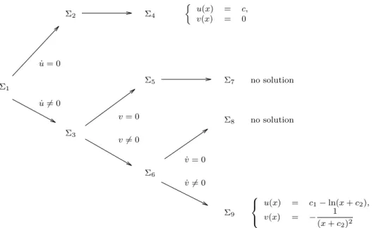
The following example is useful in Section 3.4.1. Take f = ¨u + v and A made of a single differential
polynomial p = ˙u2+ v. The leading derivative of p is ˙u. The differential polynomial f is not partially reduced
with respect to p. Differentiating, we get ˙p = 2 ˙u ¨u + ˙v. The pseudodivision of f by ˙p computes the following
relation. The differential polynomial g is the partial remainder of f by p. 2 ˙u |{z} h (¨u + v) | {z } f = |{z}1 q × (2 ˙u ¨u + ˙v)| {z } ˙ p + (2 v ˙u− ˙v) | {z } g . (17)
Proposition 11 Let A⊂ R \F be a finite set of differential polynomials, f ∈ R be a differential polynomial and g = partialrem(f, A). Then g is partially reduced with respect to A and there exists a power product h of the separants of A such that
h f = g mod [A] . (18)
The full remainder of f by A, denoted fullrem(f, A), is defined as follows. Denote A = {p1, . . . , pr},
1. if f is reduced with respect to all elements of A then fullrem(f, A) = f else
2. if f is not partially reduced with respect to A then fullrem(f, A) = fullrem(partialrem(f, A), A) else 3. there must exist some index i ∈ [1, r] such that deg(f, vi) ≥ deg(pi, vi) where vi denotes the
lead-ing derivative of pi. Among all such indices i, fix the maximal one. Then define fullrem(f, A) as
fullrem(prem(f, pi, vi), A).
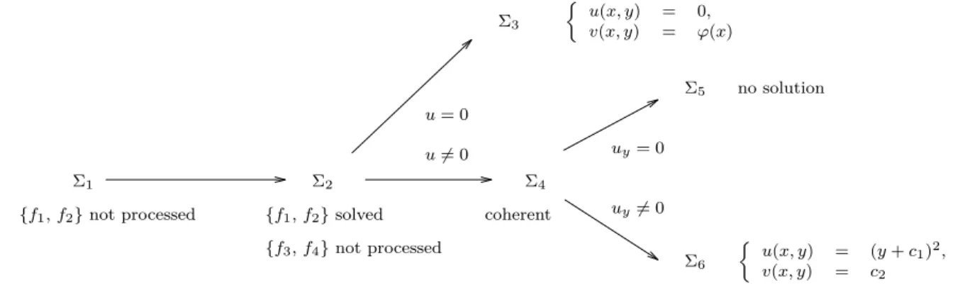
The following example is useful in Section 3.4.2. Take f = 2 u uyvxy+ 2 u2yvx− 4 ux and A = p1, p2, p3
with p1= u2y− 4 u, p2= ux− vxu and p3 = vy. The leading derivatives are uy, ux and vy. The reduction
of f is achieved by three pseudodivisions. The full remainder is g3. The power product h = h1h2h3= 1.
1 |{z} h1 × (2 u uyvxy+ 2 u2yvx− 4 ux) | {z } f = 2 u uy | {z } q1 vxy |{z} δxp3 + 2 u2yvx− 4 ux | {z } g1 , 1 |{z} h2 × (2 u2 yvx− 4 ux) | {z } g1 = |{z}2 vx q2 (u2y− 4 u) | {z } p1 + 8 u v| x{z− 4 ux} g2 , (19) 1 |{z} h3 × (8 u vx− 4 ux) | {z } g2 = |{z}−4 q3 × (ux− vxu) | {z } p2 + 4 u v| {z }x g3 .
Proposition 12 Let A⊂ R \F be a finite set of differential polynomials, f ∈ R be a differential polynomial
and g = fullrem(f, A). Then g is reduced with respect to A and there exists a power product h of the initials and the separants of A such that
h f = g mod [A] . (20)
2.3
Characteristic Sets of Prime Differential Ideals
Consider a prime differential ideal P different fromR. Assume a ranking is fixed and a characteristic set A
of P is known.
Proposition 13 Let f be any differential polynomial ofR. Then fullrem(f, A) = 0 if and only if f ∈ P. Proof Denote g = fullrem(f, A). The implication ⇐ from right to left. Assume f ∈ P. Since A ⊂ P we
have g ∈ P by the relation (20) of Proposition 12. The differential polynomial g cannot belong to R \ F
by Corollary 2, since it is reduced with respect to all elements of A. It cannot be a nonzero element of F
because P̸= R. Thus g = 0.
The implication ⇒ from left to right. Assume g = 0. Then the product h f ∈ P. By Corollary 2, the
initials and separants of A do not belong to P since they are reduced with respect to all elements of A. Since h is a power product of these initials and separants and P is prime, we have f ∈ P. □
The following notations are defined in [12, chap. 0, 1; and chap. I, 9]. In Kolchin’s book, the notation [A] : HA∞seems to occur for the first time in [12, chap. IV, 9, Lemma 2].
If S is a subset and A is an ideal of R then A : S∞ is the ideal of the elements p∈ R such that, for
some power product h of elements of S, we have h p ∈ A (if A is a differential ideal, so is A : S∞). An alternative definition is provided by means of a localization [13, chap. II, 3]: if M denotes the multiplicative family generated by S and M−1A denotes the ideal generated by A in the localized ring M−1R, then A : S∞= M−1A∩ R.
Denote now HA the set of the initials and separants of A. Proposition 13 implies that, if A is a
charac-teristic set of a prime differential ideal P then
2.4
The Ritt-Raudenbush Basis Theorem
The differential polynomial ring isR = F {u1, . . . , un}. The two next propositions are slight adaptations of
[17, chap. I, 10].
Proposition 14 Let f, g be two differential polynomials and A be a perfect differential ideal ofR such that f g∈ A. Then, for all derivative operators θ, φ, the product (θf) (φg) ∈ A.
Proof The proof is by induction on the sum of the orders of the derivative operators θ and φ. The basis
of the induction (case of two operators of order zero) holds by assumption. Assume that the Proposition holds for all derivative operators θ, φ such that the sum of their orders is equal to some positive integer and consider any derivation operator δ. Then, differentiating (θf ) (φg), we have (δθf ) (φg) + (θf ) (δφg) ∈ A
Multiply by θf and use the fact that (θf ) (φg) ∈ A (induction hypothesis). Then (θf)2(δφg) ∈ A and,
since A is perfect, (θf ) (δφg)∈ A. The fact that (δθf) (φg) ∈ A is proved similarly. □
Following [17, chap. I, 9], in order to reduce possible confusion on the meaning of curly braces, if p is a differential polynomial and Σ is a set, we will often denote Σ + p the set obtained by adjoining p to Σ.
Proposition 15 Let f, g be two differential polynomials and Σ be a set of differential polynomials of R. Then{Σ + f g} = {Σ + f} ∩ {Σ + g}.
Proof The inclusion ⊂ is clear. Let us prove the converse one. Let h ∈ {Σ + f} ∩ {Σ + g}. Then there
exists differential polynomials p, q ∈ [Σ], f ∈ [f], g ∈ [g] and, by Proposition 1, a positive integer t such
that ht = p + f and ht = q + g. Multiply these two equalities termwise. Then there exists a differential
polynomial r∈ [Σ] such that h2t= r + f g. Since f ∈ [f] and g ∈ [g], there exists finitely many differential
polynomials mθ,φ such that
f g = ∑
θ,φ∈Θ
mθ,φ (θf ) (φg) .
The product f g∈ {Σ + f g}. Thus, by Proposition 14, every product (θf) (φg) ∈ {Σ + f g}. Thus we have
h∈ {Σ + f g}. □
The remaining part of this section comes from [17, chap. I, 12-16]. Let Σ be an infinite subset of R. A
subset Φ of Σ is said to be a basis of Σ if Φ is finite and Σ⊂ {Φ}.
Lemma 2 Let Σ be an infinite subset ofR. If Σ contains a nonzero element of F then Σ has a basis.
Proof Let a be any nonzero element of Σ∩ F . Then the set {a} is a basis of Σ. □
Theorem 1 (Ritt-Raudenbush Basis Theorem) Every infinite subset ofR has a basis.
Proof We assume that there exists infinite subsets of R with no basis and seek a contradiction. Let Σ be
such a subset and assume moreover that, among all infinite sets with no basis, Σ is such that its characteristic sets are minimal.
Let A be a characteristic set of Σ.
“Perform” Ritt’s full reduction algorithm, with respect to A, over all q ∈ Σ \ A. For each q ∈ Σ \ A,
there exists a power product hq of initials and separants of A and a differential polynomial gq, reduced with
respect to A such that
Introduce the two following sets (the plus sign standing for “union”): Λ = {hqq| q ∈ Σ \ A} + A ,
Ω = {gq| q ∈ Σ \ A} + A .
The set Ω must have a basis. Indeed, if it contains any nonzero element ofF it has a basis by Lemma 2.
Otherwise, since the differential polynomials gq are reduced with respect to A, its characteristic sets are
lower than A by Proposition 10 thus it cannot lack a basis by the minimality assumption on Σ.
Thus there exists finitely many differential polynomials q1, . . . , qt ∈ Σ \ A such that the set Φ = {gq1, . . . , gqt} + A is a basis of Ω (observe that is is always possible to enlarge a basis with finitely many
further differential polynomials).
Claim: the set Ψ ={hq1q1, . . . , hqtqt} + A is a basis of Λ.
Each hqiqi− gqi (1 ≤ i ≤ t), belongs to the perfect differential ideals {Φ} and {Ψ} by Proposition 12
and the fact that A is a subset of both Φ and Ψ.
Thus, since each gqi ∈ Φ (1 ≤ i ≤ t), we see that each hqiqi∈ {Φ} (1 ≤ i ≤ t) and Ψ ⊂ {Φ}. Conversely,
since each hqiqi ∈ Ψ, we see that each gqi ∈ {Ψ} and Φ ⊂ {Ψ}. Thus both perfect differential ideals {Φ}
and{Ψ} are equal.
Since Φ is a basis of Ω we have Ω⊂ {Φ}. Since the full remainder gq of each q∈ Σ belongs to Ω, we see
that the corresponding product hqq of each q∈ Σ belongs to {Ω}, which is included in {Φ} = {Ψ}. Thus
Λ⊂ {Ψ} and the claim is proved.
Let f1, . . . , fsdenote the initials and separants of A. By Lemma 3, there exists an index 1≤ i ≤ s such
that the set Σ + fi has no basis. The differential polynomial fi∈ F by Lemma 2. Thus the set Σ + f/ ihas a
characteristic set lower than A by Proposition 10. This contradiction with the minimality assumption on Σ completes the proof of the Theorem. □
The next Lemma is involved in the proof of the Ritt-Raudenbush Basis Theorem. The differential polynomials fi actually are the initials and separants of some characteristic set of Σ.
Lemma 3 Let Σ be an infinite subset ofR and f1, . . . , fsbe differential polynomials of R. Let
Λ = {hqq| q ∈ Σ and hq is some power product of f1, . . . , fs} .
If Σ has no basis and Λ has a basis then at least one of the sets Σ + fi, for 1≤ i ≤ s, has no basis.
Proof We assume that all sets Σ + fi (1≤ i ≤ s) have a basis and seek a contradiction.
Let Ψ = {hq1q1, . . . , hqtqt} be a basis of Λ. Since a basis can always be enlarged as long as it remains
finite, there exists some finite set Φ ⊂ Σ such that: 1) Φ + fi is a basis of Σ + fi (1 ≤ i ≤ s) and; 2) q1, . . . , qt∈ Φ. Let g denote the product f1· · · fs.
By Proposition 15, the perfect differential ideal {Σ + g} is the intersection of the perfect differential
ideals{Σ + fi} (1 ≤ i ≤ s) ; similarly, the perfect differential ideal {Φ + g} is the intersection of the perfect
differential ideals{Φ + fi}. Since each Φ + fi is a basis of Σ + fi we have {Σ + g} = s ∩ i=1 {Σ + fi} ⊂ s ∩ i=1 {Φ + fi} = {Φ + g} . Thus Φ + g is a basis of Σ + g.
Thus, for each differential polynomial p∈ Σ, there exists a relation
pd = r + m1θ1g +· · · + meθeg
where d≥ 1, e ≥ 0, the mi are differential polynomials ofR and r ∈ [Φ]. Multiplying by p we get
Since q1, . . . , qt ∈ Φ we have Ψ ⊂ {Φ}. Since, moreover, p ∈ Σ and g is the product of the fi, we have p g∈ {Λ} ⊂ {Ψ} ⊂ {Φ}. Thus, by Proposition 15, we have p θig∈ {Φ} for 1 ≤ i ≤ e. Since r ∈ [Φ] we have r p∈ {Φ}. Thus, using (22), we have p ∈ {Φ}, which means that Φ is a basis of Σ: the sought contradiction.
□
Corollary 3 Let A be a perfect differential ideal ofR. Then there exists a finite Φ ⊂ A such that A = {Φ}.
Theorem 2 Every perfect differential ideal A is a finite intersection of prime differential ideals.
Proof We assume that there exists some perfect differential ideal A with no such presentation and seek a
contradiction. The perfect differential ideal A thus cannot be prime. Let f, g be two differential polynomials such that the product f g∈ A but f, g /∈ A. By Proposition 14 we have A = {A + f} ∩ {A + g}. At least one
of these two perfect differential ideals — say A1={A + f} — is not a finite intersection of prime differential
ideals; and we have A⊊ A1. Repeating this argument, we see that there exists an infinite sequence of perfect
differential ideals
A⊊ A1⊊ A2⊊ · · · (23)
Let Ω be the union of all these ideals. By the Ritt-Raudenbush Basis Theorem, there exists a finite set Φ⊂ Ω such that Ω ⊂ {Φ}. The set Φ must be a subset of some Atin (23). Thus At+1⊂ {Φ} ⊂ At. This
contradiction with the fact that the inclusions of (23) are strict completes the proof of the Theorem. □ Let A be a perfect differential ideal ofR. A representation
A = P1∩ · · · ∩ Pϱ (24)
of A as an intersection of prime differential ideals Pi is said to be minimal if, for all indices 1 ≤ i, j ≤ ϱ
such that i̸= j we have Pi ̸⊂ Pj. Anticipating on Theorem 3, these prime differential ideals are uniquely
defined. Ritt calls them the essential prime divisors of A [17, chap. I, 17]. We prefer to call them the
essential components of A.
Theorem 3 There exists a unique minimal representation of a perfect differential ideal A as a finite
inter-section of prime differential ideals.
Proof The existence comes from Theorem 2.
For the uniqueness, fix some representation (24). It suffices to prove that if P is a prime differential ideal such that A⊂ P then there exists some index 1 ≤ i ≤ ϱ such that Pi ⊂ P. If this were not the case then
each Pi would contain some differential polynomial fi such that fi ∈ P (1 ≤ i ≤ ϱ). Since P is prime, the/
product f = f1· · · fϱ would not belong to P either. However, it would belong to A. This contradiction with
the hypothesis A⊂ P completes the proof of the Theorem. □
The following example comes from [17, chap. II, 8].
{ ˙u2− 4 u} = [ ˙u2− 4 u , ¨u − 2] ∩ [u] .
The differential polynomial ˙u2− 4 u is irreducible but its first derivative actually factors as 2 ˙u (¨u − 2). The
perfect differential ideal on the left hand side of (25) is not prime. It has two essential components, given on the right hand side of (25). The solution of the first component is the family of parabolas (x + c)2 where c
is an arbitrary constant. The solution of the second component is the zero function. The singleton ˙u2− 4 u
is a characteristic set of the prime differential ideal [ ˙u2− 4 u , ¨u − 2].
A variant comes from [17, chap II, 19]. The perfect differential ideal generated by ˙u2− 4 u3 is actually
prime. Its solution is the family of functions (x + c)−2 where c is an arbitrary constant. The zero function also is a solution but (quoting Ritt) “we see, letting|c| increase, that a differential polynomial which vanishes
for every (x + c)−2vanishes for u = 0. Thus u = 0 is in the general solution”. The prime differential ideal [u] is not an essential component of{ ˙u2− 4 u3}. See also [12, chap. IV, 15, Remark 1].
2.5
Zeros of a Prime Differential Ideal
This section is much inspired by papers of Seidenberg. See the proof of [19, Theorem 6].
The differential polynomial ring isR = F {u1, . . . , un} endowed with m derivations. Since we are going to
solve polynomial systems and look for solutions inF , there are constraints on F . The content of this section
is valid if F is a universal field extension of the field Q of the rational numbers (i.e. if F is algebraically
closed and has an infinite transcendence degree overQ) [23, chap. VI, 5bis]. To fix ideas, we may consider thatF is the field C of the complex numbers.
Consider a prime differential ideal P different from R. Assume a ranking is fixed and a characteristic
set A of P is known. Denote p1, . . . , pr the elements of A and assume p1<· · · < pr.
Denote X the finite set of the derivatives A depends on, including the extra differential indeterminates used to encode the “independent variables” in the extended system associated to A, in the sense of Sec-tion 1.4.3.
Denote V ⊂ X the set of leading derivatives of A. Then ΘU \ ΘV denotes the possibly infinite set of
the elements of ΘU which are not the derivative of any element of V . Let Θ∗ denote the set of all proper derivative operators. Then Θ∗V denotes the set of all derivatives which are proper derivatives of some
element of V . The three sets V, ΘU\ ΘV and Θ∗V are pairwise disjoint. Their union is ΘU .
Process. The following process defines an expansion point and a tuple of arcs a.
1. Solve the following system as a nondifferential polynomial system ofF [X], where h denotes the product of the initial and separants of A
p1=· · · = pr= 0 , h̸= 0 .
2. Assign any value from F to the derivatives of ΘU \ ΘV and to the “independent variables” encoding
differential indeterminates which were not already assigned values at Step 1.
3. Let v be any element of Θ∗V . By Ritt’s partial reduction process, compute a power product h of
separants of A and a differential polynomial g such that
h v = g mod [A] . (25)
Then assign to v the value of g/h. A few remarks:
• the polynomial system to be solved at Step 1 is triangular in the sense that each equation pi = 0
introduces at least one indeterminate;
• if the fieldF is the field of the complex numbers, which is algebraically closed, the polynomial system to be solved has solutions;
• since the differential indeterminates which encode the “independent variables” belong to X, the con-straint h̸= 0 may forbid some expansion points;
• at the end of Step 2, the expansion point is fixed;
• at Step 3, the differential polynomials h and g depend on derivatives which were assigned values at Steps 1 and 2.
As an example, let us consider the differential polynomial p = x2u + x ˙¨ u− 2 u from Section 1.6,
for-mula (14). We have X = {x, u, ˙u, ¨u} and V = {¨u} and ΘU \ ΘV = ∅. The system of F [x, u, ˙u, ¨u] to be
solved at Step 1 is
x2u + x ˙¨ u− 2 u = 0 , x ̸= 0 .
The constraint thus imposes that the first coordinate x0of the arc x = (x0, 1, 0, . . .) assigned to x is different
comes from the polynomial (13) which has no positive integer solution. Thus, as seen in Section 1.6, the differential polynomial p has a formal power series for x0= 0. In summary, the system to be solved at Step 1
may forbid more expansion points than necessary.
Proposition 16 The tuple of arcs a or equivalently the formal power series Ψ(a) defined by the above process
provides a zero of the prime differential ideal P.
Proof The proof is by induction on the leading derivative v of the differential polynomials f∈ P, ordered
by the ranking. This transfinite induction [22, chap. 9, 4] is allowed by Proposition 6.
Basis. Thanks to Proposition 13, the elements f ∈ P with lowest leading derivative satisfy h f = q p1
where h is a power of the initial of p1(the lowest element of A) and q is some differential polynomial. Since p1
is annihilated by a and h is not, the differential polynomial f must vanish.
General case. Let v be the leading derivative of some f ∈ P. Assume (induction hypothesis) that every
element of P with leading derivative less than v is annihilated by a. We may assume, without loss of generality, that the initial of f does not belong to P. Thus, thanks to Proposition 13, we must have v∈ ΘV .
Subcase 1. Assume v ∈ V . Perform Ritt’s full reduction algorithm over f. Then there exists a power
product h of initials and separants of A such that h f ∈ [A] by Propositions 12 and 13. Observe now that, in
this reduction process, the first pseudodivision is performed with respect to the differential polynomial pi∈ A
with leading derivative v. The following pseudodivisions are performed with respect to differential polyno-mials of ΘA with leading derivatives strictly less than v; and the differential polynomial h does not depend either on any derivative greater than or equal to v. Removing all the elements of ΘA which are annihi-lated according to the induction hypothesis, we see that there exists a differential polynomial q such that
h f = q pi. Since pi is annihilated by a and h is not, the differential polynomial f must vanish.
Subcase 2. Assume v ∈ Θ∗V and that there is a single differential polynomial pi ∈ A, with leading
derivative vi such that, for some θ∈ Θ∗, we have v = θvi.
Consider Ritt’s partial reduction (25) which yielded the value of v. In this reduction process, the first pseudodivision is performed with respect to θpiand since the differential polynomial to be reduced is a mere
derivative, the first pseudoquotient is 1. Then, argumenting as in Subcase 1 and removing all the elements of ΘA which are annihilated according to the induction hypothesis, we see that h v = g + θpi. Since the
value assigned to v is g/h, we see that θpi vanishes at a.
Perform now Ritt’s full reduction algorithm over f . Then there exists a power product h of initials and separants of A such that h f ∈ [A] by Proposition 12. Argumenting as in Subcase 1 and removing all
the elements of ΘA which are annihilated according to the induction hypothesis, we see that there exists a differential polynomial q such that h f = q θpi. Since θpi is annihilated by a and h is not, the differential
polynomial f must vanish.
Subcase 3. Assume v∈ Θ∗V and that there exist many different (say two) differential polynomials pi, pj∈ A, with leading derivatives vi, vj such that, for some θi, θj∈ Θ∗, we have v = θivi = θjvj.
One of these two differential polynomials (say pi) was used to assign a value to v. As proved in Subcase 2,
the differential polynomial θipi is annihilated by a.
Denote siand sj the separants of pi and pj. The cross derivative sjθipi− siθjpj belongs to P and either
is zero or has a leading derivative strictly less than v. Thus it is annihilated by a, according to the induction hypothesis. Since θipiis annihilated and the separants are not, the differential polynomial θjpj must vanish
also.
Perform now Ritt’s full reduction algorithm over f . Argumenting as in Subcase 2, we see that f must vanish at a also. □
In the proof of the next Proposition, some fieldD is introduced. This field seems to be a field of definition,
which is a notion introduced in [12, chap. III, 3].
Proposition 17 Let f be a differential polynomial and P be a prime differential ideal of R.
Proof The idea of the proof consists in proving that P has a generic (or general) zero i.e. a zero which
only annihilates the elements of P. A zero a is generic ifF (a) is isomorphic to the field of fractions of R/P.
See [22, chap. 16].
In the field of fractions ofR/P, the derivatives in ΘU \ ΘV are transcendental over F . This is an easy
corollary to Proposition 13. Moreover, the process described at the beginning of this section for building a zero of P shows that, for every derivative v∈ ΘV , the set (ΘU \ ΘV ) + v is algebraically dependent over F inR/P. Thus ΘU \ ΘV provides a transcendence basis of the field of fractions of R/P over F .
In order to obtain a zero a of P which does not annihilate f , it is thus sufficient to assign to the derivatives in ΘU\ ΘV , values which are transcendental over F .
The issue (solved below) is that the coordinates of a belong toF thus cannot be transcendental over F .
Perform Ritt’s full reduction algorithm over f using some characteristic set A of P. Then, by Propo-sition 12, there exists a power product h of initials and separants of A and differential polynomials g, mi,θ
such that
h f = g + ∑
1≤ i ≤ r,
θ∈ Θ
mi,θ θpi.
Since Ritt’s reduction algorithm is “rational”, the above formula holds in any differential polynomial ring
D{u1, . . . , un} such that D contains the rational numbers plus the finitely many coefficients of f and the
elements of the characteristic set A. We can thus choose forD a finite extension of the field of the rational
numbers, over which the fieldF has an infinite degree of transcendency.
Thus, assigning values inF which are transcendental over D to the derivatives in ΘU \ ΘV , we obtain
a generic zero a of the prime differential ideal P∩ D{u1, . . . , un}. Since f, g /∈ P, they do not belong
to P∩ D{u1, . . . , un} either so that they are not annihilated by a. In the differential polynomial ring R, the
zero a is no more generic but it still does not annihilate f , which is the result we are looking for. □
2.6
A Differential Theorem of Zeros
Let F be a universal extension of the field of the rational numbers. To fix ideas, one may let F be the
field C of the complex numbers. Let R = F {u1, . . . , un} endowed with m derivations. Let us stress that,
in the statement of the next Theorem, the expansion points of the solutions depend on the solutions. With other words, we are looking for solutions in the ring of formal power seriesF [[x1− x1,0, . . . , xm− xm,0]] for
unspecified x1,0, . . . , xm,0 ∈ F . As pointed out in Section 1.4.3, we may also consider that the expansion
point is the origin, provided that the differential system under consideration is assumed to be “extended”.
Theorem 4 (Differential Theorem of Zeros) Let p1 =· · · = pr = 0 be a system of polynomial differential equations and f be a differential polynomial ofR. Let A = {p1, . . . , pr} be the perfect differential ideal of R generated by the left hand sides of the equations.
If f ∈ A then f annihilates over every solution of the system of equations. Conversely, if every solution of the system of equations annihilates f then f ∈ A.
Proof The first statement is clear and is valid for any fieldF . For the second statement, we assume f /∈ A
and prove that the system of equations has a solution which does not annihilate f . By Theorem 3, there exists a prime differential ideal P such that A⊂ P and f /∈ P. By Proposition 17, the prime differential
ideal P has a zero which does not annihilate f . This zero is a solution of the system of equations. □ The Theorem implies that a system has no solution if and only if 1 ∈ A where A denotes the perfect
differential ideal that generated by the system. As we shall see in the next section, there exists an algorithm which decides if 1 ∈ A. Thus the Theorem would be false if the expansion point were fixed to (say) the origin since, otherwise, we would have a contradiction with Denef and Lipshitz undecidability result.