HAL Id: tel-01998089
https://hal.archives-ouvertes.fr/tel-01998089
Submitted on 6 Mar 2019HAL is a multi-disciplinary open access archive for the deposit and dissemination of sci-entific research documents, whether they are pub-lished or not. The documents may come from teaching and research institutions in France or abroad, or from public or private research centers.
L’archive ouverte pluridisciplinaire HAL, est destinée au dépôt et à la diffusion de documents scientifiques de niveau recherche, publiés ou non, émanant des établissements d’enseignement et de recherche français ou étrangers, des laboratoires publics ou privés.
with Copulas
Fei Zheng
To cite this version:
Fei Zheng. Learning and Smoothing in Switching Markov Models with Copulas. Modeling and Simulation. Ecole Centrale de Lyon, 2017. English. �NNT : 2017LYSEC66�. �tel-01998089�
pour obtenir le grade de
DOCTEUR DE L’ÉCOLE CENTRALE DE LYON Spécialité: Informatique
Learning and Smoothing in
Switching Markov Models with Copulas
dans le cadre de l’École Doctorale InfoMaths présentée et soutenue publiquement par
Fei ZHENG
Jour de soutenance: 18 December 2017
Directeur de thèse: Prof. Stéphane Derrode Co-directeur de thèse: Prof. Wojciech Pieczynski
JURY
Jean-Yves Tourneret ENSEEIHT Toulouse Examinateur Séverine Dubuisson UPMC Sorbonnes Universités Rapporteur François Roueff Telecom ParisTech Rapporteur Stéphane Derrode É́cole Centrale de Lyon Directeur de thèse Wojciech Pieczynski Telecom SudParis Co-directeur de thèse
I would like to express my sincere gratitude to all who ever supported me during my thesis preparation and my beginner-like life in a lovely country.
My deepest gratitude to my supervisor Prof. Derrode, who holds always his door open for my questions and troubles in research. His brilliant guidance, patience and hand-on attitude on science influent me and contribute a lot to the accomplishment of this thesis. I am grateful also to work with my co-supervisor Prof. Pieczynski, who magically can always point out insightful key steps and provides me construc-tive suggestions. The pleasant discussions that we had working together is the most precious thing for this research.
Besides, I could not had a happy PhD student life without my colleagues in Laboratory LIRIS who work in Ecole Centrale de Lyon. Helpless and loneliness are kept away from me by my Chinese colleagues that I take as ”relatives”: Xiao-fang, Ying, Zehua, Qinjie, Haoyu, Dongming, Boyang, Yinhang, Huaxiong, Yuxing, Wuming, as well as by Guillaume, Richard and Maxime who are my ”lunch bros”, ”language teachers” and ”humor sources”.
My sincere thanks also goes to Isabelle and Colette, who is and worked as secretaries in LIRIS, for their help on dealing with my research activities. Thanks to Prof. Chen, the former director of our lab for his kindness that made me feel at home. For my thesis, I am also profoundly grateful to my committee members, prof. Dubuisson, prof. Tourneret and prof. Roueff for their evaluation of my work with practical advises from different aspects.
My dearest parents, my every basic particles are sampled from you. However, I haven’t find any appropriate way to show how I love you. My dear friends Nan and Guang, thank you so much to be always there to listen and help me to find back the tidiness of my life that I could have been lost for much longer without you. Dear MS, thanks for the cherish stories you shared with me, and for thousands of reason I need to say thanks but just hard to list out any...
Finally, I would like to acknowledge Chinese scholarship council who financed my research.
Abstract xi
Résumé xiii
Introduction xv
1 Pairwise Markov chain and basic methods 1
1.1 Different dependences in PMC . . . 2
1.2 PMC with discrete finite state-space . . . 4
1.2.1 Optimal restoration . . . 4
1.2.2 Unsupervised restoration . . . 7
1.2.2.1 EM for Gaussian stationary case . . . 7
1.2.2.2 ICE for stationary case . . . 9
1.2.2.3 Principles for infering hidden states . . . 10
1.3 PMC with continuous state-space . . . 12
1.3.1 Restoration of continuous state-space PMC . . . 14
1.4 Conclusion . . . 15
2 Optimal and approximated restorations in Gaussian linear Markov switching models 17 2.1 Filtering and smoothing . . . 20
2.1.1 Definition of CGPMSM and CGOMSM . . . 20
2.1.2 Optimal restoration in CGOMSM . . . 22
2.1.3 Parameterization of stationary models . . . 25
2.1.3.1 Reversible CGOMSM . . . 28
2.1.4 Restoration of simulated stationary data . . . 29
2.2 EM-based parameter estimation of stationary CGPMSM . . . 34
2.2.1 EM estimation for CGPMSM with known switches . . . 36
2.2.3 Discussion about special failure case of double-EM algorithm 45
2.3 Unsupervised restoration in CGPMSM . . . 47
2.3.1 Two restoration approaches in CGPMSM . . . 48
2.3.1.1 Approximation based on parameter modification . . 51
2.3.1.2 Approximation based on EM . . . 52
2.3.2 Double EM based unsupervised restorations . . . 57
2.3.2.1 Experiment on varying switching observation means 59 2.3.2.2 Experiment on varying noise levels . . . 63
2.4 Conclusion . . . 69
3 Non-Gaussian Markov switching model with copulas 71 3.1 Generalization of conditionally observed Markov switching model . . 73
3.1.1 Definition of GCOMSM . . . 73
3.1.2 Model simulation . . . 74
3.2 Optimal restoration in GCOMSM . . . 75
3.2.1 Optimal filtering in GCOMSM . . . 76
3.2.2 Optimal smoothing in GCOMSM . . . 77
3.2.3 Examples of GCOMSM and the optimal restoration in them 78 3.2.3.1 Example 1 – Gaussian linear case . . . 79
3.2.3.2 Example 2 – non-Gaussian non-linear case . . . 83
3.3 Model identification . . . 84
3.3.1 Generalized iterative conditional estimation . . . 87
3.3.2 Least-square parameter estimation for non-linear switching model . . . 89
3.3.3 The overall GICE-LS identification algorithm . . . 91
3.4 Performance and application of the GICE-LS identification algorithm 92 3.4.1 Performance on simulated GCOMSM data . . . 93
3.4.1.1 Gaussian linear case . . . 93
3.4.1.2 Non-Gaussian non-linear case . . . 98
3.4.2 Application of GICE-LS to non-Gaussian non-linear models . 104 3.4.2.1 On stochastic volatility data . . . 104
3.4.2.2 On Kitagawa data . . . 110
3.5 Conclusion . . . 115
4 Conclusion and perspectives 117 A Maximization of the likelihood function in Switching EM 121 B Particle filter for CGPMSM 125 B.1 Particle Filter . . . 126
B.1.1 Sequential Importance Sampling . . . 127
B.1.2 Importance distribution and weight . . . 127
B.1.3 Sampling importance resampling (SIR) . . . 128
B.2 Particle Smoother . . . 129
C Margins and copulas used in this dissertation 131
D Publications 135
1.1 Restoration error ratio of all methods (average of 100 independent
experiments) . . . 12
2.1 Θ3 of series 1 (CGOMSM-R). . . 30
2.2 Θ4 of series 1 (CGOMSM-R). . . 30
2.3 Restoration result in Series 1. . . 30
2.4 Error ratio of estimated RN 1 in Series 2. . . 33
2.5 MSE of estimated XN 1 in Series 2. . . 33
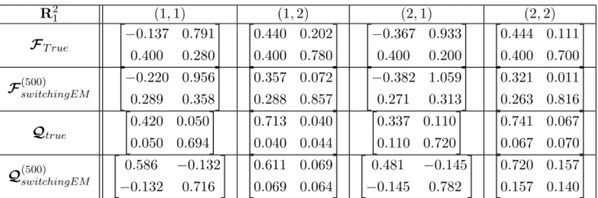
2.6 True and estimated Θ4 in experiment of Switching EM (Fyx = 0.40). 44 2.7 True and estimated Θ3 in experiment of Switching EM (Fyx = 0.40). 44 2.8 Estimated Θ1 and Θ2 in Series 2 (Fyx = 0.40). . . . 59
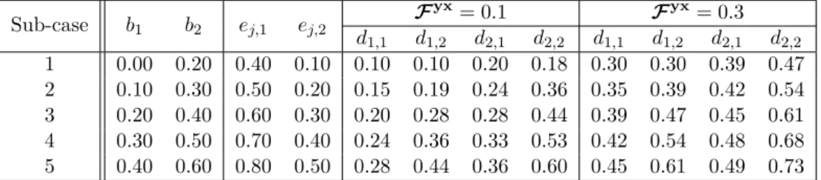
2.9 Parameters of five different noise sub-cases. . . 64
3.1 Restoration result of Example 1. . . 82
3.2 Restoration result of example 2. . . 84
3.3 Restoration results of series 1 (Gaussian linear). . . 97
3.4 Margin selection result of GICE in series 1. . . 97
3.5 Copula selection result of GICE in series 1. . . 97
3.6 Estimated parameters of p(yn+1 n rn+1n ) in series 1. . . 98 3.7 Estimated parameters of G(xn+1 xn, yn+1n , rn+1n ) in series 1. . . 98
3.8 Restoration results of series 2 (non-Gaussian non-linear). . . 101
3.9 Margin selection result of GICE in series 2. . . 102
3.10 Copula selection result of GICE in series 2. . . 102
3.11 Estimated parameters of p(yn+1 n rn+1n ) in series 2. . . 102 3.12 Estimated parameters ofG(xn+1 xn, yn+1n , rn+1n ) in series 2. . . 102
3.13 MSE results of four methods on SV model (PF represents the Particle Filter). . . 107
3.15 MSE results of four methods on KTGW model. . . 111
3.16 MSE results of ICE-LS and GICE-LS on KTGWSL model. . . 114
3.17 MSE results of CGOMSM-ABF on KTGWSL model. . . 114
C.1 Marginal distributions studied in this dissertation. . . 131
C.2 Copulas studied in this dissertation (all are one parameterized named α). . . 132
C.3 Closed-form solutions for u2 = arg max u2 ∈ [0, 1]c (u1, u2) and max (c (u1, u2)) of several copulas (u1 ∈ [0, 1]). . . 133
1.1 Dependence graphs of particular sub-models of PMC. . . 3
1.2 Error ratio tendency with iterations. . . 13
2.1 Dependence graph of CGPMSM. . . 28
2.2 Dependence graph of CGLSSM. . . 28
2.3 Dependence graph of CGOMSM. . . 29
2.4 Trajectory example of Series 1 (50 samples). . . 32
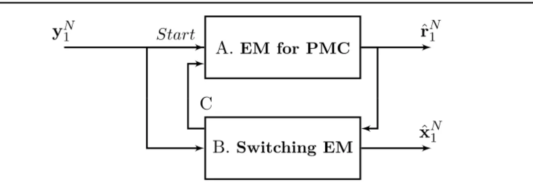
2.5 DEM-CGPMSM scheme. . . 35
2.6 Experiment of Switching EM (8 different values ofFyx). . . . 43
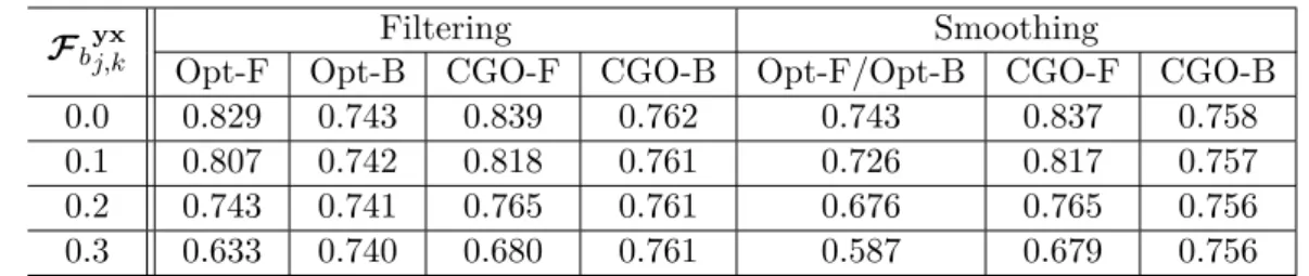
2.7 Experiment of CGPMSM filtering approaches (9 different values of Fyx). . . . 54
2.8 Experiment of CGPMSM smoothing approaches (9 different values of Fyx). . . 56
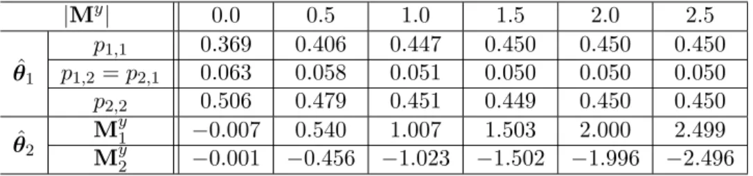
2.9 Result of restoration methods with varying|My| (Fyx= 0.20). . . . 60
2.10 Result of restoration methods with varying|My| (Fyx= 0.40). . . . 61
2.11 Error ratio of estimated switches in five different noise levels. . . 65
2.12 Restoration MSE of hidden states in five different noise levels. . . 66
2.13 Examples of a trajectory of (xN 1 , yN1 , rN1 ) (30 sample points) and restoration with OS and DEM-EM-Appro. . . 68
3.1 The distributions in Example 1. . . 80
3.2 Histograms of simulated data of Example 1 (Gaussian linear case). . 82
3.3 Trajectories of Example 1 (100 samples, Gaussian linear case). . . . 83
3.4 The distributions in Example 2. . . 85
3.5 Histograms of simulated data of Example 2 (non-Gaussian non-linear case). . . 86
3.6 Trajectories of Example 2 (100 samples, non-Gaussian non-linear case). 86 3.7 GICE-LS scheme. . . 92
3.8 The distributions of series 1 (Gaussian linear). . . 94
3.9 Trajectory example in series 1 (100 samples, smoothing). . . 99
3.10 The distributions of series 2 (non-Gaussian non-linear). . . 100
3.11 “Wrong” estimated joint distribution with (Margins: Fisk, Fisk; Cop-ula: Gumbel). . . 103
3.12 Error ratio tendency of estimated RN 1 with GICE and ICE iterations within same individual experiment in series 2. . . 103
3.13 Trajectory example in series 2 (100 samples, smoothing). . . 104
3.14 Trajectory example of SV model (60 samples, K=5). . . 109
3.15 Trajectory example of ASV model (60 samples, K=7). . . 110
3.16 Trajectory example of KTGW model (60 samples, K=7). . . 112
Switching Markov Models, also called Jump Markov Systems (JMS), are widely used in many fields such as target tracking, seismic signal processing and finance, since they can approach non-Gaussian non-linear systems. A considerable amount of related work studies linear JMS in which data restoration is achieved by Markov Chain Monte-Carlo (MCMC) methods. In this dissertation, we try to find alter-native restoration solution for JMS to MCMC methods. The main contribution of our work includes two parts. Firstly, an algorithm of unsupervised restoration for a recent linear JMS known as Conditionally Gaussian Pairwise Markov Switching Model (CGPMSM) is proposed. This algorithm combines a parameter estima-tion method named Double EM, which is based on the Expectaestima-tion-Maximizaestima-tion (EM) principle applied twice sequentially, and an efficient approach for smoothing with estimated parameters. Secondly, we extend a specific sub-model of CGPMSM known as Conditionally Gaussian Observed Markov Switching Model (CGOMSM) to a more general one, named Generalized Conditionally Observed Markov Switch-ing Model (GCOMSM) by introducSwitch-ing Copulas. ComparSwitch-ing to CGOMSM, the pro-posed GCOMSM adopts inherently more flexible distributions and non-linear struc-tures, while optimal restoration is feasible. In addition, an identification method called GICE-LS based on the Generalized Iterative Conditional Estimation (GICE) and the Least-Square (LS) principles is proposed for GCOMSM to approximate any non-Gaussian non-linear systems from their sample data set. All proposed methods are tested by simulation. Moreover, the performance of GCOMSM is discussed by application on other generable non-Gaussian non-linear Markov models, for exam-ple, on stochastic volatility models which are of great importance in finance.
Keywords: Switching Markov models, non-Gaussian non-linear Markov sys-tem, triplet Markov chain, model identification, optimal time series data restora-tion, Expectation-Maximization.
Les modèles de Markov à sauts (appelés JMS pour Jump Markov System) sont util-isés dans de nombreux domaines tels que la poursuite de cibles, le traitement des signaux sismiques et la finance, étant donné leur bonne capacité à modéliser des sys-tèmes non-linéaires et non-gaussiens. De nombreux travaux ont étudié les modèles de Markov linéaires pour lesquels bien souvent la restauration de données est réalisée grâce à des méthodes d’échantillonnage statistique de type Markov Chain Monte-Carlo (MCMC). Dans cette thèse, nous avons cherché des solutions alternatives aux méthodes MCMC et proposons deux originalités principales. La première a con-sisté à proposer un algorithme de restauration non supervisée d’un JMS particulier appelé « modèle de Markov couple à sauts conditionnellement gaussiens » (noté CGPMSM). Cet algorithme combine une méthode d’estimation des paramètres basée sur le principe Espérance-Maximisation (EM) et une méthode efficace pour lisser les données à partir des paramètres estimés. La deuxième originalité a con-sisté à étendre un CGPMSM spécifique appelé CGOMSM par l’introduction des copules. Ce modèle, appelé GCOMSM, permet de considérer des distributions plus générales que les distributions gaussiennes tout en conservant des méthodes de restauration optimales et rapides. Nous avons équipé ce modèle d’une méthode d’estimation des paramètres appelée GICE-LS, combinant le principe de la méthode d’estimation conditionnelle itérative généralisée et le principe des moindre-carrés linéaires. Toutes les méthodes sont évaluées sur des données simulées. En partic-ulier, les performances de GCOMSM sont discutées au regard de modèles de Markov non-linéaires et non-gaussiens tels que la volatilité stochastique, très utilisée dans le domaine de la finance.
chaîne de Markov triplet, identification de modèles, restauration optimale de séries temporelles de données, algorithme Espérance-Maximisation.
Time series data restoration is a common problem that we are facing in many fields. In this general problem, we are supposed to estimate the hidden sequence from an observed one, given or supposed there are some links between them. For example, in speech recognition, one wants to find out the uttered word from the given acoustic signal [55], [67], [120]; in motion detection, we are interested in discovering the real-time human activity from video or real-time sequential images [47], [104]. The Hidden Markov Model (HMM), since introduced in the late 1960s [46], [119], has become a popular statistical tool for modeling these “generative” sequences which can be characterized by an underlying process generating an observable sequence. HMM is such a class of models, assuming that the hidden states form a Markovian process, and the observations are “emitted” from the hidden states by some probability distribution. When dealing with discrete time processes, HMMs are usually called Hidden Markov Chain (HMC) as the discrete time index makes the processes like chains. Thus, concerning the applications mentioned above, two related must-be-solved problems in HMC are:
1. Restoration problem: given the observation series{y1, y2,· · · , yN}, what the most likely hidden states{x1, x2,· · · , xN} are.
2. Parameter estimation problem: under the case that the model parameters Θ are unknown, how we figure out the suitable Θ of the applied HMC.
For restoration problem, the most popular two methods are the forward-backward algorithm [120] and the Viterbi one [134], [122]. The forward-forward-backward algorithm refers to p (xn|yn1) and p
( xn yN1
)
, which are the posterior marginals of all hidden state variables given the observations, while the Viterbi algo-rithm aims to find the most likely sequence based on the maximization of
p (x1, . . . , xN, y1, . . . , yN). Two conditions can be met when dealing with the
pa-rameter estimation problem. One is to estimate the papa-rameters from observations only, for instance, maximizing p (y1, y2,· · · , yN|Θ). Most of the time we use the Baum–Welch algorithm and applies the Expectation-Maximization (EM) princi-ple to solve this parameter estimation problem with latent variables [12]. We may meet another parameter estimation occasion less tough in contrast, in which we have milder condition that sample data set which includes both hidden state samples and observation samples are given. In this case, we can simply maximize the complete data likelihood p (x1, . . . , xN, y1, . . . , yN|Θ) to figure out the suitable parameters.
With the progress of the methods for HMC, new models which generalize the classic HMC are also developed. One extension is introducing the “switch” (also called “jump”) into the HMC to characterize the time series behaviors in differ-ent regimes and permitting the change between model structures, leading to the so-called “switching Markov model” [3], [28]. The efficiency of the flexibility which benefits from this extension has been proved in targets tracking [11], [96], manu-facturing control [17] and business intelligence [41], [92]. The toughness under the switching Markov models is that most of the time, the Bayesian optimal restora-tion is no more feasible with unknown switches, so they are often approached by Markov Chain Monte-Carlo (MCMC) methods. This optimal restoration infeasi-bility also results in the hardness of parameter estimation for switching Markov models [8], [42], [90]. The other extension path of HMC enriches the dependences between the hidden states and observations. It means that the observations are no more simply “emitted” from the hidden states but have also some interactive ef-fects on the hidden process. This extension results in the “Pairwise Markov Chain” (PMC) [114], and it shows in following works on image segmentations that the consideration of interpreting these complex dependences makes sense [109], [136]. Moreover, we are pleased to apply this more general model since either restoration or parameter estimation methods of HMC can be applied with small adjustment to the PMC structure.
Recently, a fusion of these two extensions has been proposed and gave birth to a linear model known as “Conditionally Gaussian Pairwise Markov Switching Model”
(CGPMSM) [1], which thus owns both the abilities to model the switching regimes and consider more complete variable dependences. Moreover, it has a prominent merit over the other switching Markov models that the optimal restorations can be derived with specific model setting. The CGPMSM with this special setting is taken as its sub-model named “Conditionally Gaussian Observed Markov Switching Model” (CGOMSM) [1], and has been studied in [62], [61] for approximating any stationary Markov systems. Since the supervised restoration method and solution of parameter estimation with given samples are already considered in these previous works, in this dissertation, we are interested in developing the unsupervised restora-tion methods for CGPMSM. It means to find solurestora-tions for learning its parameters from only observations and conducting restorations with the learned parameters. This is one main part of our work. Also, we notice that the feasibility of optimal restoration is no need to be constrained under the Gaussian linear model structure. In fact, we can form the conditional joint distributions in switching Markov mod-els with the introduction of Copulas, which has been widely applied in the field of finance and insurance [18], [132], [49]. The Copula can be considered as a “tie” between margins, with which a joint distribution becomes easily be written in terms of univariate marginal distribution functions. It has been successfully introduced into Markov models such as the HMC and PMC [24], [37], [38], but from our best knowledge, so far, there is no work that considers the incorporation of Copulas in a switching Markov model. Inspired by this, the second main part of our work focuses on extending the CGOMSM into a more general switching Markov model by making use of Copulas. Thus, the new model can incorporate varied conditional distribution, while still allowing optimal restorations. We also consider an iterative method to solve the parameter estimation problem for the new model using sample data set, so that the model can be applicable on approaching any time independent Markov systems and to perform their data restorations.
Outline of the thesis
Chapter 1 describes the PMC model, which is the basic structure of the switching Markov models that we are going to study. Discrete and continuous state-space PMC are introduced separately with their matched methods of restoration and parameter estimation.
Chapter 2 focuses on the restoration methods of Gaussian linear Markov models (the CGPMSM family). Optimal restoration is derived for the special sub-model of CGPMSM known as CGOMSM. Then, for the unsupervised restoration of the CGPMSM, an EM principle based parameter estimation method from only obser-vations is proposed and described with details. Meanwhile, two restoration ap-proaches are presented for restoration under the general CGPMSM. The fusion of the proposed parameter estimation method and the restoration approaches leads to an unsupervised strategy whose efficiency is proved by simulations. Finally, several series of experiments are conducted to analyze the performance of the pro-posed unsupervised restoration method with comparison to supervised optimal and sub-optimal methods considering different impacting factors.
Chapter 3 contributes to build the general non-Gaussian model which allows optimal restorations inspired by the CGOMSM model. Firstly, we give the defi-nition of the proposed model (briefly denoted by GCOMSM), and the way for its simulation. Then the optimal restorations (filtering and smoothing) are derived, with two simulation examples to verify their efficiency and show the generality of the GCOMSM. Moreover, an identification method based on “Generalized Iterative Conditional Estimation” (GICE) and Least-Square (LS) called GICE-LS is pro-posed for estimating the distributions and parameters of the propro-posed model. The efficiency of GICE-LS on identification of GCOMSM is proved by simulation. Fi-nally, we apply the GCOMSM restoration identified by GICE-LS to some generable non-Gaussian non-linear systems to objectively show the merits of our algorithm comparing to the CGOMSM restoration and Particle Filter.
In the end, Chapter 4 summarizes the main contributions of this dissertation, presents some limitations in the proposed methods which can be improved, and draws an outlook for possible future work.
Pairwise Markov chain and
basic methods
Since proposed in [114], Pairwise Markov Chain (PMC) arouses more and more attention as a generalization of Hidden Markov Chain (HMC). Playing the same role, replacing the classic HMC, the PMC has been applied to signal and image processing fields, such as speech recognition [87], image segmentation or classifica-tion [34], [35], [109], [136]. All these works show that the PMC brings improvements on result thanks to its consideration of more complex dependence between stochas-tic variables.
We will introduce and detail the properties of PMC in this Chapter. In section 1.1, we explain its sub-cases of different dependences between variables. Focus on the restoration of the hidden states in PMC, we consider both discrete finite space case and continuous case in Section 1.2 and Section 1.3. Supervised and unsupervised restoration solutions for these PMC models are given. Meanwhile, the frequently used Gaussian PMCs are discussed, and some results of different restoration solutions are illustrated for discrete finite space case.
Let us consider two sequences of random variables. RN
1 = (R1, R2, . . . , RN),
each Rn takes its value in a set R; and YN1 = (Y1, Y2, . . . , YN), each Yn takes
its value in a set Y . Both the spaces R and Y can be discrete or continuous. We note further HN
1 = (H1, H2. . . , HN), where Hn= (Rn, Yn), and rN1 , yN1 , hN1 for
the realization of RN
1 , YN1 and HN1 respectively. Then, the process HN1 is a PMC
if it holds the Markov property that
p(hN
1
)
1.1
Different dependences in PMC
There could be varying dependences inside a PMC structure, as we can decompose the transition probability of PMC into
p (hn+1|hn) = p ( rn+1, yn+1|rn, yn ) = p (rn+1|rn, yn) p ( yn+1|rn, rn+1, yn ) . (1.2)
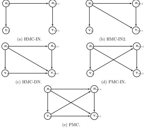
Considering the different cases in equation (1.2), we have four sub-models of PMC, each of them holds their special dependence of noise. The dependence graphs of all these sub-cases of PMC are displayed in Figure 1.1.
(a) When p (rn+1|rn, yn) = p (rn+1|rn) and p
(
yn+1|rn, rn+1, yn
) = p(yn+1|rn+1), the process HN
1 is the well recognized HMC. More precisely,
we call it “Hidden Markov Chain with Independent Noise” (HMC-IN). The transition probability in (1.2) thus becomes
p(rn+1, yn+1|rn, yn
)
= p (rn+1|rn) p
(
yn+1|rn+1). (1.3)
In this classic case, RN
1 is a Markov chain and Y1,· · · , YN are independent
from each other knowing RN
1 . (b) When p(yn+1|rn, rn+1, yn ) = p(yn+1|rn, rn+1 ) , the process HN 1 is called
“Hidden Markov Chain with Independent Noise of order 2” (HMC-IN2) with transition probability p(rn+1, yn+1|rn, yn ) = p (rn+1|rn) p ( yn+1|rn, rn+1 ) . (1.4)
RN1 is still a Markov chain, and Y1,· · · , YN are independent conditionally
on RN
1 , but the dependence on RN1 is more complicated than in HMC-IN.
HMC-IN can be seen as a particular case of this HMC-IN2.
(c) If only RN
1 is assumed Markovian, the process HN1 is called “Hidden Markov
writes p(rn+1, yn+1|rn, yn ) = p (rn+1|rn) p ( yn+1|rn, rn+1, yn ) . (1.5)
Under this case, Y1,· · · , YN become dependent from each other conditionally
on RN
1 , and obviously, this is a more general case than the last two cases.
Rn Rn+1 Yn Yn+1 (a) HMC-IN. Rn Rn+1 Yn Yn+1 (b) HMC-IN2. Rn Rn+1 Yn Yn+1 (c) HMC-DN. Rn Rn+1 Yn Yn+1 (d) PMC-IN. Rn Rn+1 Yn Yn+1 (e) PMC.
Figure 1.1: Dependence graphs of particular sub-models of PMC.
(d) Here we consider RN
1 no more Markovian, and Y1,· · · , YN independent
con-ditionally on RN
1 , which means that
p(rn+1, yn+1|rn, yn ) = p (rn+1|rn, yn) p ( yn+1|rn, rn+1 ) (1.6)
This special case is called “Pairwise Markov Chain with Independent Noise” (PMC-IN), and if we call the most general PMC the “Pairwise Markov Chain with Dependent Noise” (PMC-DN), in which all dependences are conserved,
the PMC-IN is its sub-case. Later if no confusion will be introduced, “PMC” will refer to the PMC-DN instead.
Let us notice that, there are a lot of works on Markov models among which some also inspired by the “pairwise” idea. In [50], [51], the PMC is called Bi-variate Markov Chain; similarly, it is called the Coupled Markov Chain or Mod-els in [21], [20], [118]; moreover, the Double Chain Markov Model discussed in [13] and [14] which is actually the HMC-DN but with p(yn+1|rn, rn+1, yn
) = p(yn+1|rn+1, yn). The novelty of PMC is the fact that RN
1 is not necessarily
Markovian, and it gives necessary and sufficient conditions for stationary time-reversible model to exist [84]. Besides, one should pay attention that these works have different emphasis. Some of them assumes RN
1 are hidden, YN1 are observed;
while the others consider the total pair HN
1 are hidden states. Also, considering
the state-space, it can be discrete classes or continues real values. One can decide where to apply the PMC and which state-space to choose according to the practical issue. In this chapter, we only discuss the case that RN
1 are hidden states and YN1
are observations.
1.2
PMC with discrete finite state-space
Let us consider the PMC with discrete finite state-space, like in classic HMC, hidden states RN
1 is a discrete process, each Rntakes its values in discrete finite state-space
Ω = {1, 2, . . . , K}; and YN1 = (Y1, Y2, . . . , YN) is a continuous observation with
each Yn taking its values in Rq, q represents the dimension of Yn. Benefiting
from the Markovianity of p(RN
1 YN1
)
, optimal restoration exists in PMC in spite weather RN
1 being Markovian or not [114], [84], [52].
1.2.1 Optimal restoration
Here we explain how the restorations (both filtering and smoothing) of PMC with discrete finite state-space run. We define that
ϕn(j) = p
(
rn= j yN1
)
ψn(j, k) = p
(
rn= j, rn+1= k yN1
)
, (1.8)
where j, k ∈ Ω. The restoration can be calculated through the forward and back-ward probabilities by Baum’s algorithm [12], [86], [40] from the structure of PMC. To iteratively compute (1.7)-(1.8), we adopt the “normalize” forward and backward probabilities [35]: αn(j) = p (rn= j|yn1) , (1.9) βn(j) = p(yN n+1|rn= j, yn ) p(yN n+1|yn1 ) . (1.10)
These definition avoid the numerical underflow problem comparing to the original one [12], which computes the forward p(yN
1 , xn= j ) and backward p(yN n+1|yn, xn= j ) recursively instead.
With the definitions above, we get forwardly the αn through
α1(j) = p (r1= j, y1) ∑ l∈Ω p (r1 = l, y1) ; αn(j) = ∑ l∈Ω αn−1(l) p ( rn= j, yn rn−1= l, yn−1 ) ∑ (l1,l2)∈Ω2 αn−1(l1) p ( rn= l2, yn rn−1= l1, yn−1 ), (1.11)
which is the probability of filtering. While backwardly, we get the intermediate elements for smoothing
βN(j) = 1; βn(j) = ∑ l∈Ω βn+1(l) p ( rn+1= l, yn+1|rn= j, yn ) ∑ (l1,l2)∈Ω2 αn(l1) p ( rn+1= l2, yn+1|rn= l1, yn ), (1.12)
where 1≤ n < N. So the smoothing probability, which is noted as ϕn(j) in (1.7)
is given by
and the joint posteriori probability ψn(j, k) is given by ψn(j, k) = αn(j) p ( rn+1= k, yn+1|rn= j, yn ) βn+1(k) ∑ (l1,l2)∈Ω2 αn(l1) p ( rn+1= l2, yn+1|rn= l1, yn ) βn+1(l2) . (1.14)
Most of the time, we deal the restoration under simple but practical assumption that the PMC is Gaussian stationary. It means that the probability of p (hn, hn+1)
does not depend on n, and therefore, the distributions p(yn, yn+1|rn, rn+1
)
, which can be written as p (y1, y2|r1, r2) are Gaussian given by:
p (h1, h2) = p (r1 = j, y1, r2= k, y2) = pj,k fj,k(y1, y2) , (1.15)
pj,k is the abbreviation of p (rn= j, rn+1= k) (we will keep using this abbreviation
though out this dissertation), and
fj,k(y1, y2) = p (y1, y2|r1 = j, r2 = k ) =N ( My21 j,k, Γ y2 1 j,k ) . (1.16) My21 j,k and Γ y2 1
j,k denote the mean and variance of the joint Gaussian distribution of
(y1, y2) conditionally on (rn= j, rn+1= k) respectively.
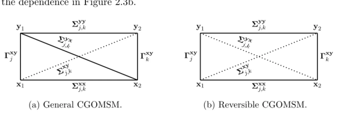
In practice, sometimes, Gaussian distribution may be not always suitable, and a flexible shape of fj,k(y1, y2) can be defined by two marginal distributions and a dependence item known as copula [29], [98], [100], [124]. So the form of fj,k(y1, y2)
writes according to this construction as
fj,k(y1, y2) = f (l) j,k(y1) f (r) k,j(y2) cj,k ( Fj,k(l)(y1) , Fk,j(r)(y2) ) , (1.17) in which fj,k(l)(y1) = f(l)(y1|rn= j, rn+1= k), fk,j(r)(y2) = f(r)(y2|rn+1 = k, rn= j)
are the two marginal densities, with (l), (r) specify the left or right margin respec-tively. The dependent structure cj,k(·, ·) is the so called “copula”, and Fj,k(l)(y1) denotes the associated Cumulative Distribution Function (CDF) of fj,k(l)(y1), and
Fk,j(r)(y2), the associated CDF of fk,j(r)(y2). More details of the copula in fj,k(y1, y2)
of PMC will be discussed later embedded in the Markov switching model which we are going to deal with in Chapter 3.
Of course, for any sub-case of PMC that has special dependence structure as described in previous Section, the restoration of the general PMC are suitable.
1.2.2 Unsupervised restoration
When applying the PMC to a real system, we have no idea what the parameters of a suitable PMC are. In this case, we often turn to the well known Expectation-Maximization (EM) principle for solution.
EM is an iterative method for searching maximum likelihood (ML) estimates of parameters in statistical models, when parts of the variables are missing (latent). The definition of EM principle was explained in [33], [97], but there are earlier works on this iterative method for exponential families [129], [128], [127], published as pointed out in [33]. The convergence of EM in [33] is revised by [135] later.
Back to the PMC that we are dealing with, (rN
1 , yN1
)
is considered as the com-plete data for likelihood calculation, while rN
1 is latent, so the unsupervised Bayesian
restoration based on ML can be handled with EM as already dealt in [82], [121] ex-tended from the solution of HMC discussed in [123], [25]. It is necessary to mention that EM algorithm works well when the system is stationary. Otherwise, the unsu-pervised restoration would loss its efficiency, since it can only recover the stationary PMC which models the system.
1.2.2.1 EM for Gaussian stationary case
As proposed in [82], the EM method estimates the parameters of stationary Gaus-sian PMC by maximizing the likelihood function of incomplete data YN
1 iteratively
according to
Θh(i+1)= arg max
Θh EΘh(i) [ ln pΘh ( HN 1 ) yN1 ] , (1.18) with Θh = ( pj,k, M y2 1 j,k, Γ y2 1 j,k )
, 1≤ j, k ≤ K and the index i denotes the EM iteration.
(M-Step) iteratively run as follows:
1) E-step:
E-step calculates the expectation of the likelihood with current parameters Θh(i) (estimated from last M-step) which is actually simplified to get the update of ψn(j, k) in (1.8). The computation is just the same as the optimal smoothing
of this discrete state-space PMC which has been specified from equations (1.7) to (1.14).
2) M-step:
Then, the M-step searches to maximize (1.18) by taking derivative with respect to each parameter, which gives the following update equations for all the parameters:
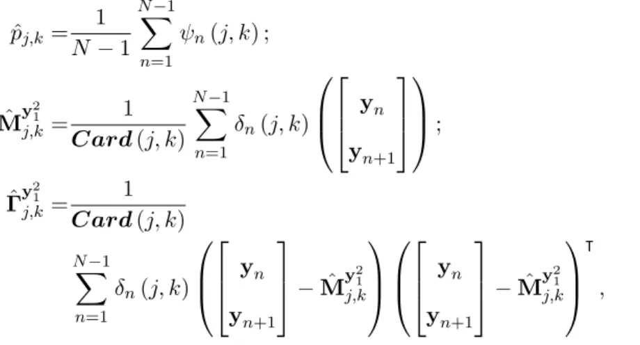
ˆ pj,k= 1 N− 1 N∑−1 n=1 ψn(j, k) ; ˆ My21 j,k= N∑−1 n=1 ψn(j, k) yn yn+1 N∑−1 n=1 ψn(j, k) ; ˆ Γy 2 1 j,k= N∑−1 n=1 ψn(j, k) yn yn+1 − ˆMy 2 1 j,k yn yn+1 − ˆMy 2 1 j,k ⊺ N∑−1 n=1 ψn(j, k) . (1.19)
To initialize the iterations, one simple way is to use K-means clustering method to find the initial switches RN
Θh(0) by empirical estimations: ˆ pj,k = Card (j, k) N − 1 ; ˆ My21 j,k = 1 Card (j, k) N∑−1 n=1 δn(j, k) yn yn+1 ; ˆ Γy 2 1 j,k = 1 Card (j, k) N∑−1 n=1 δn(j, k) yn yn+1 − ˆMy21 j,k yn yn+1 − ˆMy21 j,k ⊺ . (1.20)
in which δn(j, k) denotes the function 1 (rn= j, rn+1 = k), and Card (j, k) =
∑N−1
n=1 δn(j, k). There are also some other initialization methods which could be
applied as discussed and compared in [15].
Finally, EM is stopped after the change of the likelihood between two iterations is considered small enough (one can set a threshold to specify the convergence).
1.2.2.2 ICE for stationary case
When it comes to non-Gaussian case, direct derivative of parameters from the form of ML may be complex or not possible. As an alternative method, “iterative conditional estimation” (ICE) was proposed by [113] for solving the fundamental limitation of EM. It uses also the complete data HN
1 , but the computation of the
likelihood is not necessary. The efficiency and convergence of ICE have been verified with application in statistical image segmentation by [83], [111], [19] and [31].
ICE assumes that there exists an estimator for HN
1 denoted by ˆΘ h( HN 1 ) = ˆ Θh(RN 1 , YN1 )
with hidden data RN
1 that one wants to recover. The
natu-ral best estimator, which considers the minimum mean square error denoted by EΘh [ ˆ Θh(HN 1 ) yN1 ]
is a conditional expectation on Θh. While Θh is unknown, we can have iterative method to approach it
Θh(i+1)=EΘh(i) [ ˆ Θh(HN 1 ) yN1 ] . (1.21)
We see that, when ˆΘh is chosen to be an ML estimator, equation (1.21) becomes Θh(i+1)=EΘh(i) [ arg max Θh ln pΘh ( HN 1 ) yN1 ] , (1.22)
which is identical to EM if the expectation and the log-likelihood maximization can be exchanged, and this occurs when the distribution of complete data belongs to an exponential family. Therefore, EM algorithm can be taken as a particular case of ICE for this kind of canonical parameterization structures. More discussion about the equivalence of ICE and EM can be found in [32].
The advantage of ICE is that, if we can compute the conditional distribution of (
RN
1 |yN1
)
at step i but not the expectation in (1.21) analytically, we can simulate the realization rN 1 of RN1 according to p ( RN 1 yN1 )
, with the current parameter Θh(i) (it is called the Random Imputation Principle (RIP) in [27]), and then θi+1
can be approximated empirically, thanks to the law of large numbers as
Θh(i+1)= 1 M [ ˆ Θh(rN 1 ) 1+ ˆΘ h( rN 1 ) 2+· · · + ˆΘ h( rN 1 ) M ] , (1.23) where (rN 1 ) 1,· · · , ( rN 1 ) M areM realizations of RN1 .
Let us pay attention that, there is another similar simulation based alternative method for EM, which is called stochastic EM (SEM) [99], [85], [95], [27]. SEM takes realization (stochastic) step after E-step only once, and M-step which defining Θh(i+1)is given by solve the ML function with the realized complete data. We can see that, SEM is also a special case of ICE when M = 1 and ML is chosen to be the ˆΘh.
1.2.2.3 Principles for infering hidden states There are several criterions to infer the hidden RN
1 from the filtering probabilities
p (rn|yn1) and smoothing ones p
( rn yN1
)
. The MPM (Maximum Posterior Mode) criterion, which maximizes the posteriors is commonly used according to the com-putation of
ˆ
rn= arg max j
with j ∈ Ω for n from {1, · · · , N}. And another Bayesian criterion often used is the MAP (Maximum A Posteriori estimation) defined as a regularization of ML estimation by the prior of p(yN
1 ) that ˆ rN 1 = arg max rn∈Ω p(rN 1 , yN1 ) . (1.25)
In this dissertation, we always use MPM to obtain the restoration of RN
1 due to its
simplicity.
We address here an experiment to show the performance of unsupervised restora-tion methods on HMC-DN as a groundwork, since it is a partial structure of the switching Markov models we deal with later.
As defined in HMC-DN, RN
1 is Markov, and we set each Rn adopts simply two
possible values, which means that Ω ={1, 2}. The probabilities of RN
1 , which has
already appeared in (1.15) are defined by p1,2= p2,1 = 0.05 and p1,1= p2,2 = 0.45.
The dependence of p(yN
1 rN1
)
is set to be Gaussian with the auto-regressive relation
Yn+1=Fyy(Rn+1 n ) Yn+Byy(Rn+1 n ) Vn+1, (1.26)
in which Vn+1 is a standard normal white noise written as Vn+1 ∼ N (0, 1), and initially, the Y1 ∼ N (0, 1) also. The parameters Fyy
( Rn+1 n ) and Byy(Rn+1 n ) are assigned as Fyy(Rn= 0, Rn+1 = 0) = Fyy(Rn= 1, Rn+1= 0) = 0.4, Fyy(R n= 0, Rn+1= 1) = Fyy(Rn= 1, Rn+1 = 1) = 0.9 and Byy(Rn, Rn+1) = √
1− Fyy(Rn, Rn+1)2. Under this setting, we have the conditional means of
(
yn, yn+1|rn, rn+1
)
all 0, variance all 1, and the covariance cov(yn, yn+1|rn, rn+1
) = Fyy(r
n, rn+1). 2000 samples are simulated according to the model setting, then,
the supervised filtering, smoothing, and unsupervised smoothing through EM and ICE are applied on the observations for restoration. In particular, the ICE applied here adopts the classic empirical estimation of the moments as ˆΘh, based on hidden
state realizations rN
1 , and M set to one in (1.23), which runs
ˆ pj,k = 1 N− 1 N∑−1 n=1 ψn(j, k) ; ˆ My21 j,k = 1 Card (j, k) N∑−1 n=1 δn(j, k) yn yn+1 ; ˆ Γy 2 1 j,k = 1 Card (j, k) N∑−1 n=1 δn(j, k) yn yn+1 − ˆMy21 j,k yn yn+1 − ˆMy21 j,k ⊺ , (1.27)
where δn(j, k) and Card (j, k) are defined the same as in (1.20).
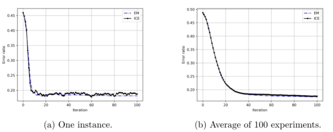
The average result of 100 Monte-Carlo experiments are reported in Table 1.1 As EM and ICE make use of the entire YN
1 , we only report their smoothing result
in the Table. The error ratio tendencies of EM and ICE of both one instance and average of 100 independent experiments are displayed in figure 1.2. We find that with estimator based on realization, ICE is more fluctuating than EM, but the two algorithms perform nearly the same under the setting of this experiment. The fluctuation may be smoothen with the increasing value of M which is only set to 1 in this example.
Table 1.1: Restoration error ratio of all methods (average of 100 independent ex-periments) .
Optimal filtering Optimal smoothing EM ICE
Error Ratio 0.196 0.173 0.189 0.180
1.3
PMC with continuous state-space
The continuous state-space PMC has the hidden state takes its value in a continuous real space. To distinguish it from the discrete state-space PMC, we take XN
1 =
(X1, X2,· · · , XN) instead of RN1 to denote the values of hidden state, where each
Xn takes its value inRs, and “s” being the dimension of X n.
(a) One instance. (b) Average of 100 experiments. Figure 1.2: Error ratio tendency with iterations.
particular Gaussian linear case, which is called “Linear Gaussian Pairwise Markov Model” [116] or “Gaussian Pairwise Markov Model” (GPMM) [1], written as
Xn+1 Yn+1 = F xx n+1 F xy n+1 Fyxn+1 F yy n+1 | {z } Fn+1 Xn Yn + B xx n+1 B xy n+1 Byxn+1 B yy n+1 | {z } Bn+1 Un+1 Vn+1 , (1.28)
in whichFn+1andBn+1are parameters of the regime. Wn+1=
[
U⊺n+1, V⊺n+1]⊺are noises which follow independently the standard normal distribution, and are inde-pendent of X1, Y1. Under Gaussian assumption that X1, Y1 and W1are all
Gaus-sian, the pair (XN
1 , YN1
)
is then a Gaussian process. Consequently, p (xn+1|yn1),
p (xn|yn1), p
( xn yN1
)
are all Gaussian.
The continuous state-space Gaussian linear HMC known as Hidden Gaussian Markov Model (HGMM) [4], [9], [77] is often written in the form
Xn+1= An+1Xn+ Bn+1Un+1;
Yn+1= Cn+1Xn+1+ Dn+1Vn+1,
(1.29)
with matrices An+1, Bn+1, Cn+1, Dn+1 defining the linear functions. Un+1, Vn+1 are standard normal white noises which are independent from each other and inde-pendent from X1and Y1. However, as HMC is a sub-model of PMC, spontaneously, HGMM is a sub-model of GPMM. Just with some parameters set to be 0, HGMM
can be rewritten as Xn+1 Yn+1 = F xx n+1 0 Fyx n+1 0 | {z } Fn+1 Xn Yn + B xx n+1 0 Byx n+1 B yy n+1 | {z } Bn+1 Un+1 Vn+1 , (1.30) where Fxxn+1 = An+1, Fyxn+1= Cn+1An+1,Bxxn+1 = Bn+1,Byxn+1 = Cn+1Bn+1, and Byy n+1= Dn+1. As in PMC, the hidden X N
1 in GPMM can be Markov or not [84].
1.3.1 Restoration of continuous state-space PMC
The optimal restoration for the continuous state-space PMC in general way can be derived by the following steps.
One step ahead prediction:
p (xn+1|yn1) =
∫
p (xn+1|xn, yn) p (xn|yn1) dxn, (1.31)
so the forward filtering is
p(xn+1 yn+11 ) = p ( xn+1, yn+1|yn1 ) p(yn+1|yn 1 ) = ∫ p(xn+1, yn+1|xn, yn ) p (xn|yn1) dxn ∫ p(yn+1|xn, yn ) p (xn|yn1) dxn . (1.32)
Benefit from the pairwise structure, we have
p(xn xn+1, yn+11
)
= p(xn xn+1, yN1
)
, (1.33)
and the backward smoothing can be reached by
p(xn yN1 ) = ∫ p(xn, xn+1 yn+11 ) p(xn+1 yn+11 ) p(xn+1 yN1 ) dxn+1 = ∫ p (x n|yn1) p ( xn+1, yn+1|xn, yn1 ) p(yn+1|yn)p(xn+1 yn+1 1 ) p(xn+1 yN 1 ) dxn+1 = p (xn|yn1) ∫ p(x n+1, yn+1|xn, yn1 ) p(xn+1 yN1 ) p(xn+1, yn+1|yn 1 ) dxn+1 , (1.34)
with p(xn+1, yn+1|yn1)= ∫ p (xn|yn1) p ( xn+1, yn+1|xn, yn ) dxn. (1.35)
Then (1.31)-(1.34) are computable in Gaussian case.
The unsupervised restoration based on EM for GPMM has been developed by [5] and the robustness strengthened by [101] through QR decompositions. Moreover, a partial supervised solution is given by [102]. As we will depict the extension model of GPMM with switches in next chapter, GPMM will become its sub-case with zero switch. For not duplicating the state of method, the unsupervised restoration of GPMM can be referred in next Section removing the switch symbols.
1.4
Conclusion
This chapter presents the principle of Pairwise Markov Chains (PMCs) and their restoration algorithms, whatever supervised or unsupervised based on Expectation-Maximization (EM) and Iterative Conditional Estimation (ICE) principles for pa-rameter estimation. The PMC is a generalization of the classic Hidden Markov Chain (HMC). Definition, property and advantage of PMC are described in de-tails in the beginning of this chapter. Two cases of hidden states (discrete finite and continuous) in PMC are specified then, with the derivation of both supervised and unsupervised restorations. In addition, an example of unsupervised restoration of the discrete finite state-space PMC is reported to show the performance of all restoration methods on the commonly used Gaussian case.
PMC is the basic of the switching Markov model we handle in this thesis. Ac-tually, the special switching Markov model we are going to deal with, is a Triplet Markov Chain (TMC) [117] developed from the GPMM (Gaussian continuous state-space PMC) with essential consideration of switching regime. In practice, this “switching” regime makes the Markov chain owns the ability to describe the dra-matic change of the auto-regression and better suits for approaching the non-linear systems. This chapter paves the way for finding the solution of the main subject
which we are facing to and the methods described will be the reference of the new methods we developed for switching Markov models in following chapters.
Optimal and approximated
restorations in Gaussian linear
Markov switching models
As described in previous Chapter, the simplest model for the distribution of (XN1 , YN1 ) which allows fast Bayesian linear processing, is the classic HGMM de-fined by Gaussian distribution p (x1) of X1, the Markov transitions p (xn+1|xn) and
simple dependence p (yn|xn). The HGMM has been later extended to GPMM
de-fined by Gaussian distribution p (x1, y1) of (X1, Y1) and the pairwise Markov
tran-sitions p(xn+1, yn+1|xn, yn
)
. Optimal filtering and smoothing remains workable in GPMM, while comparing to HGMM, it incorporates more complex dependence between the stochastic variables.
Let us now extend the previous models by introducing a hidden process to model the “switches” (also called “jumps”). We consider XN
1 ={X1, X2, . . . , XN},
RN
1 = {R1, R2, . . . , RN}, and YN1 = {Y1, Y2, . . . , YN}, each Xn, Rn, Yn takes
its value in Rs, Ω = {1, 2, . . . , K}, and Rq respectively. YN
1 is observed, and the
problem is to estimate the hidden realizations of XN
1 from only YN1 . Introducing
discrete switches RN
1 in the plain models mentioned before is of interest for at least
two aspects. Firstly, this can model stochastic regime changes. It is to say that it allows random changes in the parameters which define the plain HGMM and GPMM. Secondly, when we consider a Markov triplet TN
1 = (XN1 , RN1 , YN1 ) such
that (XN
1 , YN1 ) is a GPMM conditionally on RN1 , the distribution of (XN1 , YN1 )
be-comes a Gaussian mixture distribution, which is likely to approximate non-Gaussian non-linear systems. Such situation has been successfully considered in [62], where
it shows that stationary or asymptomatically stationary Markov system can be ap-proximated by a Gaussian switching system once a method to simulate realizations of the system is available.
Introducing discrete switches RN
1 in the classic HGMM leads to the following
Conditionally Gaussian Linear State-space Model (CGLSSM) [26]:
RN
1 is Markov,
Xn+1= An+1(Rn+1)Xn+ Bn+1(Rn+1)Un+1,
Yn+1= Cn+1(Rn+1)Xn+1+ Dn+1(Rn+1)Vn+1.
(2.1)
An+1(Rn+1), Bn+1(Rn+1), Cn+1(Rn+1), Dn+1(Rn+1) are matrices conditionally on
Rnof dimension s× s, s × s, q × s and q × q respectively. Un+1, Vn+1 are random
variables distributed according to standard Normal distribution. The CGLSSM is also known as “Linear system with jump parameters” [133]; “Switching Linear Dy-namic Systems” [77], [125]; “Jump Markov Linear Systems” [7]; “Switching Linear State-space Models” [6]; and “Conditional Linear Gaussian Models” [93] applied in tracking, speech feature mapping and biomedical engineering, etc.
While RN
1 is hidden, in CGLSSM, computing conditional mean estimates of
hidden states is infeasible as it involves a cost that grows exponentially with the number of observations [115]. The restoration is often approached by Markov Chain Monte-Carlo (MCMC) methods [42], [43]. When it comes to the unsupervised case, recent works on the parameter estimation of CGLSSM or the more general Jump Markov System (JMS), combine EM with Sequential Monte-Carlo (SMC) methods to do the parameter estimation [54], [108]. As MCMC methods can approximate properly the target distribution with large sample numbers, the restoration per-formance can be quite satisfactory. However, the computational consumption of MCMC based methods increases with sample numbers when high accuracy is re-quired and can meet degeneracy problems [71], [64].
We consider the recent model extended from CGLSSM, called Conditionally Gaussian Pairwise Markov Switching Model (CGPMSM) [1], which introduces the switches RN
esti-mation method only from the observed YN
1 for stationary CGPMSM, and perform
unsupervised restoration without making use of the MCMC methods. The remain-ing of this chapter is organized as follows. In Section 2.1, we recall the definition of the special JMLS family called CGPMSM which we are interested in. Next, we derive the optimal filtering and smoothing of the “Conditionally Gaussian Ob-served Markov Switching Model” (CGOMSM), which is a sub-model of CGPMSM. Then, for the restoration of general stationary CGPMSM, which will be discussed in following Sections, we detail its parameterizations. Two experimental series on simulated data are conducted in this Section to verify the supervised filtering and smoothing for CGOMSM, and their ability to restore the close CGPMSM as sub-optimal solution. Section 2.2 extends the EM algorithm for parameter estimation in GPMM to Switching EM which works on parameter estimation on CGPMSM with known switches. Then, a parameter estimation method for CGPMSM with unknown switches called Double EM is proposed, which applies twice the EM prin-ciple incorporating the Switching EM. Meanwhile, the shortcoming of the proposed Double EM is also pointed out. Section 2.3 proposes two restoration approaches in CGPMSM, one is with partial mild modification of parameters and the other is based on EM principle. Then, several unsupervised strategies are produced by fus-ing the Double EM parameter estimation and restoration approaches. Two Series of experiments focus on different observation means and varying noise levels are conducted to test the proposed Double EM method and study the performance of all proposed unsupervised restoration methods with comparison to several existing supervised restoration methods under the influence of these two factors. Finally, the work of this Chapter is concluded in Section 2.4.
2.1
Filtering and smoothing
2.1.1 Definition of CGPMSM and CGOMSM
The CGPMSM is a switching Gaussian linear dynamic stochastic system defined by: TN 1 = (XN1 , RN1 , YN1 ) is Markov with p (rn+1|xn, rn, yn) = p (rn+1|rn) , (2.2) Xn+1− M x n+1(Rn+1) Yn+1− Myn+1(Rn+1) | {z } Zn+1−Mzn+1 = F xx n+1(Rn+1n ) F xy n+1(Rn+1n ) Fyx n+1(Rn+1n ) F yy n+1(Rn+1n ) | {z } Fn+1(Rn+1n ) Xn− M x n(Rn) Yn− Myn(Rn) | {z } Zn−Mzn + B xx n+1(Rn+1n ) B xy n+1(Rn+1n ) Byx n+1(Rn+1n ) B yy n+1(Rn+1n ) | {z } Bn+1(Rn+1n ) Un+1 Vn+1 | {z } Wn+1 . (2.3) X1, Y1, R1 are given following Gaussian distribution p (x1, y1|r1) and p (r1)
respectively. The hidden switches RN
1 is a Markov chain, which comes from
p (rn+1|xn, rn, yn) = p (rn+1|rn). UN1 and VN1 note the mutually independent
centered Gaussian noise with unit variance-covariance matrix which are also as-sumed independent from RN
1 . The system parametersFn+1(rn+1n ) andBn+1(rn+1n )
depend on the switches rn+1
n = (rn, rn+1)1, so the couple (XN1 , YN1 ) is Markovian
and Gaussian conditionally on RN
1 . Mxn(rn) and Myn(rn) are the means of Xn
and Yn conditionally on rn, we denote Mzn(rn) = [Mnx(rn), Myn(rn)]⊺. The original
model defined by [1] does not consider Mxn(rn) and Myn(rn), or we can say they are
set to be both zero. (2.3) can be concisely written as
Zn+1− Mzn+1(Rn+1) =Fn+1(Rn+1n ) (Zn− Mzn(Rn)) +Bn+1(Rn+1n )Wn+1. (2.4)
Like HGMM can be taken as a special case under GPMM. Under the general family of CGPMSM, the classic CGLSSM without the consideration of means can
be represented by setting several zeros and simplifying the correspondence on switch to the present state of Rn+1 in the (2.3).
Xn+1 Yn+1 | {z } Zn+1 = F xx n+1(Rn+1) 0 Fyx n+1(Rn+1) 0 | {z } Fn+1(Rn+1) Xn Yn | {z } Zn + B xx n+1(Rn+1) 0 Byx n+1(Rn+1) Byyn+1(Rn+1) | {z } Bn+1(Rn+1) Un+1 Vn+1 | {z } Wn+1 . (2.5) Compare to the classic CGLSSM (2.1), we have the congruent relationship:
Fxx n+1(Rn+1) = An+1(Rn+1); Fyx n+1(Rn+1) = Cn+1(Rn+1)An+1(Rn+1); Bxx n+1(Rn+1) = Bn+1(Rn+1); Byx n+1(Rn+1) = Cn+1(Rn+1)Bn+1(Rn+1); Byyn+1(Rn+1) = Dn+1(Rn+1). (2.6) Conditionally on RN
1 , XN1 is linear Gaussian and Markovian, and the distribution
of YN
1 conditionally to XN1 is simple in CGLSSM. Thus given RN1 = rN1 , the
couple (XN
1 , YN1 ) degenerates as a HGMM, in which the classical optimal Kalman
filter and smoother can be applied. But in case that RN
1 is unknown, although
CGLSSM appears as “natural” switching Gaussian system, neither optimal filtering nor smoothing can be derived.
Of course, the general CGPMSM extended from GPMM also meets this tough problem. But let us pay attention to the pairwise structure of CGPMSM. Actually, the observations and hidden states play symmetrical roles, we can take arbitrarily any of these two as the other’s noisy version. If we inverse the roles of XN
1 and YN1
in CGLSSM, both p(rn xN1
)
and p(yn rn, xN1
)
become computable. Based on this idea, the sub-family of CGPMSM named “Conditionally Gaussian Observed Markov Switching Model” (CGOMSM) has also been proposed in [1], [2]. The CGOMSM is with a fixed Fyxn+1(Rn+1n ) = 0 in CGPMSM verifying that: