HAL Id: hal-01360166
https://hal.archives-ouvertes.fr/hal-01360166
Submitted on 20 Sep 2016
HAL is a multi-disciplinary open access
archive for the deposit and dissemination of
sci-entific research documents, whether they are
pub-lished or not. The documents may come from
teaching and research institutions in France or
abroad, or from public or private research centers.
L’archive ouverte pluridisciplinaire HAL, est
destinée au dépôt et à la diffusion de documents
scientifiques de niveau recherche, publiés ou non,
émanant des établissements d’enseignement et de
recherche français ou étrangers, des laboratoires
publics ou privés.
Semantic Segmentation of Earth Observation Data
Using Multimodal and Multi-scale Deep Networks
Nicolas Audebert, Bertrand Le Saux, Sébastien Lefèvre
To cite this version:
Nicolas Audebert, Bertrand Le Saux, Sébastien Lefèvre. Semantic Segmentation of Earth
Observa-tion Data Using Multimodal and Multi-scale Deep Networks. Asian Conference on Computer Vision
(ACCV16), Nov 2016, Taipei, Taiwan. �10.1007/978-3-319-54181-5_12�. �hal-01360166�
Data Using Multimodal and Multi-scale Deep
Networks
Nicolas Audebert1,2, Bertrand Le Saux1, S´ebastien Lef`evre2
1
ONERA, The French Aerospace Lab, F91761 Palaiseau, France -{nicolas.audebert,bertrand.le saux}@onera.fr
2Univ. BretagneSud, UMR 6074, IRISA, F56000 Vannes, France
Abstract. This work investigates the use of deep fully convolutional neural networks (DFCNN) for pixel-wise scene labeling of Earth Obser-vation images. Especially, we train a variant of the SegNet architecture on remote sensing data over an urban area and study different strategies for performing accurate semantic segmentation. Our contributions are the following: 1) we transfer efficiently a DFCNN from generic everyday images to remote sensing images; 2) we introduce a multi-kernel convo-lutional layer for fast aggregation of predictions at multiple scales; 3) we perform data fusion from heterogeneous sensors (optical and laser) using residual correction. Our framework improves state-of-the-art accuracy on the ISPRS Vaihingen 2D Semantic Labeling dataset.
1
Introduction
Over the past few years, deep learning has become ubiquitous for computer vi-sion tasks. Convolutional Neural Networks (CNN) took over the field and are now the state-of-the-art for object classification and detection. Recently, deep networks extended their abilities to semantic segmentation, thanks to recent works designing deep networks for dense (pixel-wise) prediction, generally built around the fully convolutional principle stated by Long et al. [1]. These archi-tectures have gained a lot of interest during the last years thanks to their ability to address semantic segmentation. Indeed, fully convolutional architectures are now considered as the state-of-the-art on most renowned benchmarks such as PASCAL VOC2012 [2] and Microsoft COCO [3]. However, those datasets focus on everyday scenes and assume a human-level point of view. In this work, we aim to process remote sensing (RS) data and more precisely Earth Observation (EO) data. EO requires to extract thematic information (e.g. land cover us-age, biomass repartition, etc.) using data acquired from various airborne and/or satellite sensors (e.g. optical cameras, LiDAR). It often relies on a mapping step, that aims to automatically produce a semantic map containing various regions of interest, based on some raw data. A popular application is land cover mapping where each pixel is assigned to a thematic class, according to the type of land
cover (vegetation, road, . . . ) or object (car, building, . . . ) observed at the pixel coordinates. As volume of EO data continuously grows (reaching the Zettabyte scale), deep networks can be trained to understand those images. However, there are several strong differences between everyday pictures and EO imagery. First, EO assumes a bird’s view acquisition, thus the perspective is significantly altered w.r.t. usual computer vision datasets. Objects lie within a flat 2D plane, which makes the angle of view consistent but reduces the number of depth-related hints, such as projected shadows. Second, every pixel in RS images has a seman-tic meaning. This differs from most images in the PASCAL VOC2012 dataset, that are mainly comprised of a meaningless background with a few foreground objects of interest. Such a distinction is not as clear in EO data, where im-ages may contain both semantically meaningful “stuff” (large homogeneous non quantifiable surfaces such as water bodies, roads, corn fields, . . . ) and “objects” (cars, houses, . . . ) that have different properties.
First experiments using deep learning introduced CNN for classification of EO data with a patch based approach [4]. Images were segmented using a seg-mentation algorithm (e.g. with superpixels) and each region was classified using a CNN. However, the unsupervised segmentation proved to be a difficult bot-tleneck to overcome as higher accuracy requires strong oversegmentation. This was improved thanks to CNN using dense feature maps [5]. Fully supervised learning of both segmentation and classification is a promising alternative that could drastically improve the performance of the deep models. Fully convolu-tional networks [1] and derived models can help solve this problem. Adapting these architectures to multimodal EO data is the main objective of this work.
In this work, we show how to perform competitive semantic segmentation of EO data. We consider a standard dataset delivered by the ISPRS [6] and rely on deep fully convolutional networks, designed for dense pixel-wise prediction. Moreover, we build on this baseline approach and present a simple trick to smooth the predictions using a multi-kernel convolutional layer that operates several parallel convolutions with different kernel sizes to aggregate predictions at multiple scale. This module does not need to be retrained from scratch and smoothes the predictions by averaging over an ensemble of models considering multiple scales, and therefore multiple spatial contexts. Finally, we present a data fusion method able to integrate auxiliary data into the model and to merge predictions using all available data. Using a dual-stream architecture, we first naively average the predictions from complementary data. Then, we introduce a residual correction network that is able to learn how to fuse the prediction maps by adding a corrective term to the average prediction.
2
Related Work
2.1 Semantic Segmentation
In computer vision, semantic segmentation consists in assigning a semantic label (i.e. a class) to each coherent region of an image. This can be achieved using pixel-wise dense prediction models that are able to classify each pixel of the
image. Recently, deep learning models for semantic segmentation have started to appear. Many recent works in computer vision are actually tackling semantic segmentation with a significant success. Nearly all state-of-the-art architectures follow principles stated in [1], where semantic segmentation using Fully Con-volutional Networks (FCN) has been shown to achieve impressive results on PASCAL VOC2012. The main idea consists in modifying traditional classifica-tion CNN so that the output is not a probability vector but rather a probability map. Generally, a standard CNN is used as an encoder that will extract fea-tures, followed by a decoder that will upsample feature maps to the original spatial resolution of the input image. A heat map is then obtained for each class. Following the path opened by FCN, several architectures have proven to be very effective on both PASCAL VOC2012 and Microsoft COCO. Progresses have been obtained by increasing the field-of-view of the encoder and removing pooling layers to avoid bottlenecks (DeepLab [7] and dilated convolutions [8]). Structured prediction has been investigated with integrated structured models such as Conditional Random Fields (CRF) within the deep network (CRFas-RNN [9,10]). Better architectures also provided new insights (e.g. ResNet [11] based architectures [12], recurrent neural networks [13]). Leveraging analogies with convolutional autoencoders (and similarly to Stacked What-Where Au-toencoders [14]), DeconvNet [15] and SegNet [16] have investigated symmetrical encoder-decoder architectures.
2.2 Scene Understanding in Earth Observation Imagery
Deep learning on EO images is a very active research field. Since the first works on road detection [17], CNN have been successfully used for classification and dense labeling of EO data. CNN-based deep features have been shown to out-perform significantly traditional methods based on hand-crafted features and Support Vector Machines for land cover classification [18]. Besides, a framework using superpixels and deep features for semantic segmentation outperformed traditional methods [4] and obtained a very high accuracy in the Data Fusion Contest 2015 [19]. A generic deep learning framework for processing remote sensing data using CNN established that deep networks improve significantly the commonly used SVM baseline [20]. [21] also performed classification of EO data using ensemble of multiscale CNN, which has been improved with the in-troduction of FCN [22]. Indeed, fully convolutional architectures are promising as they can learn how to classify the pixels (“what”) but also predict spatial structures (“where”). Therefore, on EO images, such models would be not only able to detect different types of land cover in a patch, but also to predict the shapes of the buildings, the curves of the roads, . . .
3
Proposed Method
3.1 Data Preprocessing
High resolution EO images are often too large to be processed in only one pass through a CNN. For example, the average dimensions of an ISPRS tile from
Vaihingen dataset is 2493× 2063 pixels, whereas most CNN are tailored for
a resolution of 256× 256 pixels. Given current GPU memory limitations, we
split our EO images in smaller patches with a simple sliding window. It is then possible to process arbitrary large images in a linear time. In the case where consecutive patches overlap at testing time (if the stride is smaller than the patch size), we average the multiple predictions to obtain the final classification for overlapping pixels. This smoothes the predictions along the borders of each patch and removes the discontinuities that can appear.
We recall that our aim is to transpose well-known architectures from tra-ditional computer vision to EO. We are thus using neural networks initially designed for RGB data. Therefore, the processed images will have to respect such a 3-channel format. The ISPRS dataset contains IRRG images of Vaihin-gen. The 3 channels (i.e. near-infrared, red and green) will thus be processed as an RGB image. Indeed, all three color channels have been acquired by the same sensor and are the consequence of the same physical phenomenon. These channels have homogeneous dynamics and meaning for our remote sensing ap-plication. The dataset also includes additional data acquired from an aerial laser sensor and consisting of a Digital Surface Model (DSM). In addition, we also use the Normalized Digital Surface Model (NDSM) from [23]. Finally, we com-pute the Normalized Difference Vegetation Index (NDVI) from the near-infrared and red channels. NDVI is a good indicator for vegetation and is computed as follows:
N DV I = IR− R
IR + R . (1)
Let us recall that we are working in a 3-channel framework. Thus we build for each IRRG image another companion composite image using the DSM, NDSM and NDVI information. Of course, such information does not correspond to color channels and cannot be stacked as an RGB color image without caution. Nev-ertheless, this composite image contains relevant information that can help dis-criminating between several classes. In particular, the DSM includes the height information which is of first importance to distinguish a roof from a road section, or a bush from a tree. Therefore, we will explore how to process these heteroge-neous channels and to combine them to improve the model prediction by fusing the predictions of two networks sharing the same topology.
3.2 Network architecture
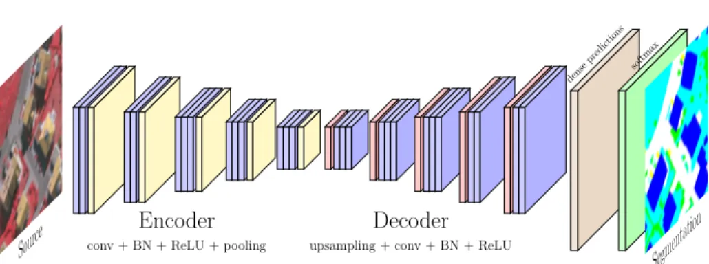
SegNet There are many available architectures for semantic segmentation. We
choose here the SegNet architecture [16] (cf. Fig. 1), since it provides a good balance between accuracy and computational cost. SegNet’s symmetrical archi-tecture and its use of the pooling/unpooling combination is very effective for precise relocalisation of features, which is intuitively crucial for EO data. In addition to SegNet, we have performed preliminary experiments with FCN [1] and DeepLab [7]. Results reported no significant improvement (or even no im-provement at all). Thus the need to switch to more computationally expensive
Source
dense predictions
softmax
Encoder
conv + BN + ReLU + poolingDecoder
upsampling + conv + BN + ReLUSegmen
tation
Fig. 1: Illustration of the SegNet architecture applied to EO data.
architectures was not demonstrated. Note that our contributions could easily be adapted to other architectures and are not specific to SegNet.
SegNet has an encoder-decoder architecture based on the convolutional layers of VGG-16 from the Visual Geometry Group [24,25]. The encoder is a succession of convolutional layers followed by batch normalization [26] and rectified linear units. Blocks of convolution are followed by a pooling layer of stride 2. The decoder has the same number of convolutions and the same number of blocks. In place of pooling, the decoder performs upsampling using unpooling layers. This layer operates by relocating at the maximum index computed by the associated pooling layer. For example, the first pooling layer computes the mask of the maximum activations (the “argmax”) and passes it to the last unpooling layer, that will upsample the feature map to a full resolution by placing the activations on the mask indices and zeroes everywhere else. The sparse feature maps are then densified by the consecutive convolutional layers. The encoding weights are initialized using the corresponding layers from VGG-16 and the decoding weights are initialized randomly using the strategy from [27]. We report no gain with alternative transfer functions such as ELU [28] or PReLU [27] and do not alter further the SegNet architecture. Let N be the number of pixels in a patch and k the number of classes, for a specified pixel i, let yi denote its label
and (zi
1, . . . , zik) the prediction vector; we minimize the normalized sum of the
multinomial logistic loss of the softmax outputs over the whole patch:
loss = 1 N N X i=1 k X j=1 yijlog exp(zi j) k P l=1 exp(zi l) . (2)
As previously demonstrated in [29], visual filters learnt on generic datasets such as ImageNet can be effectively transferred on EO data. However, we suggest that remote sensing images have a common underlying spatial structure linked to the orthogonal line of view from the sky. Therefore, it is interesting to allow the filters to be optimized according to these specificities in order to leverage the
= same weights Encoder Encoder deconv5 deconv4 deconv3 deconv2 deconv1 (3x3) deconv5 deconv4 deconv3 deconv2 deconv1 (5x5) Encoder deconv5 deconv4 deconv3 deconv2 deconv1 (7x7) Prediction small context Prediction large context
+
Prediction medium context
Multi-kernel layer
Multi-scale prediction
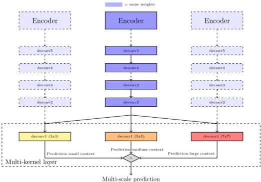
Fig. 2: Our multi-kernel convolutional layer operates at 3 multiple scales, which is equivalent to averaging an ensemble of 3 models sharing weights.
common properties of all EO images, rather than waste parameters on useless filters. To assess this hypothesis, we experiment different learning rates for the encoder (lre) and the decoder (lrd). Four strategies have been experimented:
– same learning rate for both: lrd= lre, lre/lrd= 1,
– slightly higher learning rate for the decoder: lrd= 2× lre, lre/lrd= 0.5,
– strongly higher learning rate for the decoder: lrd= 10× lre, lre/lrd= 0.1,
– no backpropagation at all for the encoder: lre= 0, lre/lrd= 0.
As a baseline, we also try to randomly initialize the weights of both the encoder and the decoder to train a new SegNet from scratch using the same learning rates for both parts.
Multi-kernel Convolutional Layer Finally, we explore how to take spatial
context into account. Let us recall that spatial information is crucial when deal-ing with EO data. Multi-scale processdeal-ing has been proven effective for classifi-cation, notably in the Inception network [30], for semantic segmentation [8] and on remote sensing imagery [21]. We design here an alternative decoder whose last layer extracts information simultaneously at several spatial resolutions and
aggregates the predictions. Instead of using only one kernel size of 3× 3, our
of size 3× 3, 5 × 5 and 7 × 7 with appropriate padding to keep the image dimen-sions. These different kernel sizes make possible to aggregate predictions using different receptive cell sizes. This can be seen as performing ensemble learning where the models have the same topologies and weights, excepted for the last layer, as illustrated by Fig. 2. Ensemble learning with CNN has been proven to be effective in various situations, including super-resolution [31] where mul-tiple CNN are used before the final deconvolution. By doing so, we are able to aggregate predictions at different scales, thus smoothing the predictions by com-bining different fields of view and taking into account different sizes of spatial
context. If Xp denotes the input activations of the multi-kernel convolutional
layer for the pthfeature map, Zs
p the activations after the convolution at the sth
scale (s∈ {1, . . . , S} with S = 3 here), Z0
q the final outputs and Wp,qs the qth
convolutional kernel for the input map p at scale s, we have: Z0 q = 1 S S X s=1 Zs p= 1 S S X s=1 X p Ws p,qXp . (3)
Let S denote the number of parallel convolutions (here, S = 3). For a given pixel at index i, if zks,i is the activation for class k and scale s, the logistic loss after the softmax in our multi-kernel variant is:
loss = N X i=1 k X j=1 yi jlog exp(1 S S P s=1 zs,ij ) k P l=1 exp(1 S S P s=1 zs,il ) . (4)
We can train the network using the whole multi-kernel convolutional layer at once using the standard backpropagation scheme. Alternatively, we can also train only one convolution at a time, meaning that our network can be trained at first with only one scale. Then, to extend our multi-kernel layer, we can simply drop the last layer and fine-tune a new convolutional layer with another kernel size and then add the weights to a new parallel branch. This leads to a higher flexibility compared to training all scales at once, and can be used to quickly include multi-scale predictions in other fully convolutional architectures only by fine-tuning.
This multi-kernel convolutional layer shares several concepts with the com-petitive multi-scale convolution [32] and the Inception module [30]. However, in our work, the parallel convolutions are used only in the last layer to perform model averaging over several scales, reducing the number of parameters to be optimized compared to performing multi-scale in every layer. Moreover, this en-sures more flexibility, since the number of parallel convolutions can be simply extended by fine-tuning with a new kernel size. Compared to the multi-scale context aggregation from Yu and Koltun [8], our multi-kernel does not reduce dimensions and operates convolutions in parallel. Fast ensemble learning is then performed with a very low computational overhead. As opposed to Zhao et al. [21], we do not need to extract the patches using a pyramid, nor do we need
SegNet IRRG Encoder SegNet DSM/NDSM/NDVI Encoder deconv5 + BN + ReLU deconv4 + BN + ReLU deconv3 + BN + ReLU deconv2 + BN + ReLU deconv1 + BN + ReLU Prediction deconv5 + BN + ReLU deconv4 + BN + ReLU deconv3 + BN + ReLU deconv2 + BN + ReLU deconv1 + BN + ReLU Prediction + Combined predictions
(a) Averaging strategy.
SegNet IRRG Encoder SegNet DSM/NDSM/NDVI Encoder deconv5 + BN + ReLU deconv4 + BN + ReLU deconv3 + BN + ReLU deconv2 + BN + ReLU deconv1 + BN + ReLU Prediction deconv5 + BN + ReLU deconv4 + BN + ReLU deconv3 + BN + ReLU deconv2 + BN + ReLU deconv1 + BN + ReLU Prediction concat fusion network deconv + BN + ReLU (learning rate * 10) Combined predictions
(b) Fusion network strategy.
Fig. 3: Fusion strategies of our dual-stream SegNet architecture.
to choose the scales beforehand, as we can extend the network according to the dataset.
3.3 Heterogeneous Data Fusion with Residual Correction
Traditional 3-channel color images are only one possible type of remote sensing data. Multispectral sensors typically provide 4 to 12 bands, while hyperspectral images are made of a few hundreds of spectral bands. Besides, other data types such as DSM or radar imagery may be available. As stated in Section 3.1, IRRG data from the ISPRS dataset is completed by DSM, NDSM and NDVI. So we will assess if it is possible to: 1) build a second SegNet that can perform semantic segmentation using a second set of raw features, 2) combine the two networks to perform data fusion and improve the accuracy.
The naive data fusion would be to concatenate all 6 channels (IR/R/G and DSM/NDSM/NDVI) and feed a SegNet-like architecture with it. However, we were not able to improve the performance in regard to a simple IRRG architec-ture. Inspired by the multimodal fusion introduced in [33] for joint audio-video representation learning and the RGB-D data fusion in [34], we try a prediction-oriented fusion by merging the output activations maps. We consider here two strategies: 1) simple averaging after the softmax (Fig. 3a), 2) neural network merge (Fig. 3b). The latter uses a corrector network that can learn from both sets of activations to correct small deficiencies in the prediction and hopefully globally improve the prediction accuracy.
ac ti vat ion m ap s SegNet IRRG IRRG prediction SegNet composite Composite prediction F u si on co n vo lu ti on 1 F u si on co n vo lu ti on 2 F u si on co n vo lu ti on 3 correction + ×0.5 ×0.5 Corrected combined prediction
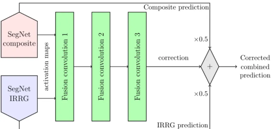
Fig. 4: Fusion network for correcting the predictions using information from two complementary SegNet using heterogeneous data.
Our original fusion network consisted in three convolutional layers which input was intermediate feature maps from the original network. More precisely, in the idea of fine-tuning by dropping the last fully connected layer before the softmax, we remove the last convolutional layer of each network and replace them by the fusion network convolutional layer, taking the concatenated intermediate feature maps in input. This allows the fusion network to have more information about raw activations, rather than just stacking the layers after the preprocessed predictions. Indeed, because of the one-hot encoding of the ground truth labels, the last layer activations tend to be sparse, therefore losing information about activations unrelated to the highest predicted class. However, this architecture does not improve significantly the accuracy compared to a simple averaging.
Building on the idea of residual deep learning [11], we propose a fusion net-work based on residual correction. Instead of dropping entirely the last convolu-tional layers from the two SegNets, we keep them to compute the average scores. Then, we use the intermediate feature maps as inputs to a 3-convolution layers “correction” network, as illustrated in Fig. 4. Using residual learning makes sense in this case, as the average score is already a good estimation of the reality. To improve the results, we aim to use the complementary channels to correct small errors in the prediction maps. In this context, residual learning can be seen as
learning a corrective term for our predictive model. Let Mrdenote the input of
the rthstream (r
∈ {1, . . . , R} with R = 2 here), Pr the output probability
ten-sor and Zrthe intermediate feature map used for the correction. The corrected
prediction is: P0(M 1, . . . , MR) = P (M1, . . . , MR) + correction(Z1, . . . , ZR) (5) where P (M1, . . . , MR) = 1 R R X r=1 Pr(Mr) . (6)
Table 1: Results on the validation set with different initialization policies.
Initialization Random VGG-16 Learning rate ratio lre
lrd 1 1 0.5 0.1 0
Accuracy 87.0% 87.2% 87.8% 86.9% 86.5%
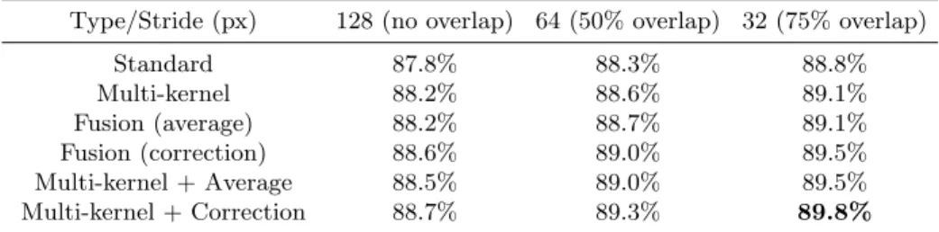
Table 2: Results on the validation set.
Type/Stride (px) 128 (no overlap) 64 (50% overlap) 32 (75% overlap) Standard 87.8% 88.3% 88.8% Multi-kernel 88.2% 88.6% 89.1% Fusion (average) 88.2% 88.7% 89.1% Fusion (correction) 88.6% 89.0% 89.5% Multi-kernel + Average 88.5% 89.0% 89.5% Multi-kernel + Correction 88.7% 89.3% 89.8%
Using residual learning should bringkcorrectionk kP k. This means that
it should be easier for the network to learn not to add noise to predictions where
its confidence is high (kcorrectionk ' 0) and only modify unsure predictions.
The residual correction network can be trained by fine-tuning as usual with a logistic loss after a softmax layer.
4
Experiments
4.1 Experimental Setup
To compare our method with the current state-of-the-art, we train a model using the full dataset (training and validation sets) with the same training strategy. This is the model that we tested against other methods using the ISPRS evalu-ation benchmark1.
4.2 Results
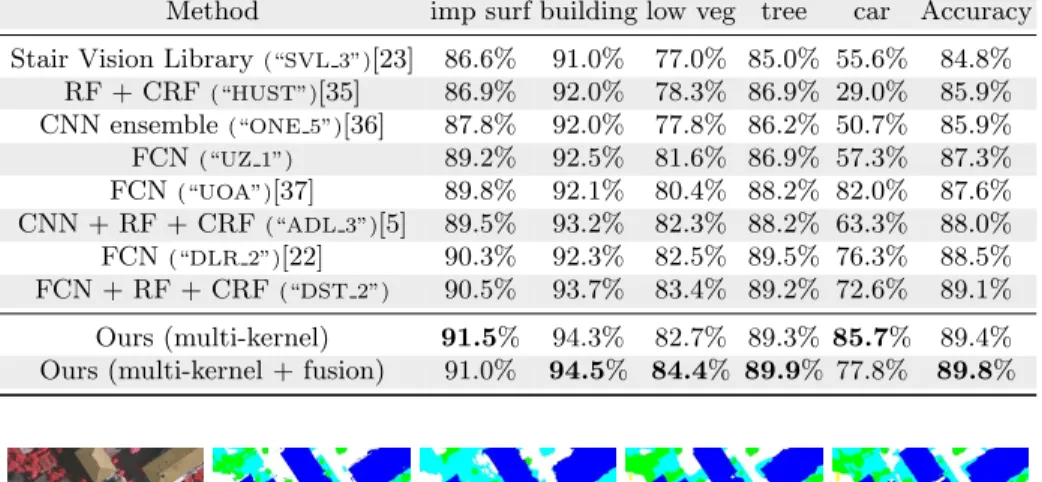
Our best model achieves state-of-the art results on the ISPRS Vaihingen dataset (cf. Table 3)2. Fig. 5 illustrates a qualitative comparison between SegNet using
our multi-kernel convolutional layer and other baseline strategies on an extract of the Vaihingen testing set. The provided metrics are the global pixel-wise accuracy and the F1 score on each class:
1 In this benchmark, the evaluation is not performed by us or any other competing
team, but directly by the benchmark organizers.
Table 3: ISPRS 2D Semantic Labeling Challenge Vaihingen results.
Method imp surf building low veg tree car Accuracy Stair Vision Library(“SVL 3”)[23] 86.6% 91.0% 77.0% 85.0% 55.6% 84.8%
RF + CRF(“HUST”)[35] 86.9% 92.0% 78.3% 86.9% 29.0% 85.9% CNN ensemble(“ONE 5”)[36] 87.8% 92.0% 77.8% 86.2% 50.7% 85.9% FCN(“UZ 1”) 89.2% 92.5% 81.6% 86.9% 57.3% 87.3% FCN(“UOA”)[37] 89.8% 92.1% 80.4% 88.2% 82.0% 87.6% CNN + RF + CRF(“ADL 3”)[5] 89.5% 93.2% 82.3% 88.2% 63.3% 88.0% FCN(“DLR 2”)[22] 90.3% 92.3% 82.5% 89.5% 76.3% 88.5% FCN + RF + CRF(“DST 2”) 90.5% 93.7% 83.4% 89.2% 72.6% 89.1% Ours (multi-kernel) 91.5% 94.3% 82.7% 89.3% 85.7% 89.4% Ours (multi-kernel + fusion) 91.0% 94.5% 84.4% 89.9% 77.8% 89.8%
IRRG data “SVL”[23] RF + CRF[35] “DLR” (FCN)[22]
Ours (SegNet)
Fig. 5: Comparison of the generated segmentations using several methods of the ISPRS Vaihingen benchmark (patch extracted from the testing set).
(white: roads,blue: buildings, cyan: low vegetation,green: trees,yellow: cars)
F 1i = 2 precisioni× recalli precisioni+ recalli and recalli= tpi Ci , precisioni= tpi Pi , (7)
where tpi the number of true positives for class i, Ci the number of pixels
belonging to class i, and Pi the number of pixels attributed to class i by the
model. These metrics are computed using an alternative ground truth in which the borders have been eroded by a 3px radius circle.
Previous to our submission, the best results on the benchmark were ob-tained by combining FCN and hand-crafted features, whereas our method does not require any prior. The previous best method using only a FCN (“DLR 1”) reached 88.4%, our method improving this result by 1.4%. Earlier methods using CNN for classification obtained 85.9% (“ONE 5”[36]) and 86.1% (“ADL 1”[5]). It should be noted that we outperform all these methods, including those that use hand-crafted features and structured models such as Conditional Random Fields, although we do not use these techniques.
IRRG data Composite data IRRG prediction IRRG prediction (multi) Composite prediction Composite prediction (multi) Ground truth
Fig. 6: Effects of the multi-kernel convolutional layer on selected patches.
4.3 Analysis
Sliding Window Overlap Allowing an overlap when sliding the window across
the tile slows significantly the segmentation process but improves accuracy, as shown in Table 2. Indeed, if we divide the stride by 2, the number of patches is multiplied by 4. However, averaging several predictions on the same region helps to correct small errors, especially around the borders of each patch, which are difficult to predict due to a lack of context. We find that a stride of 32px (75% overlap) is fast enough for most purposes and achieves a significant boost in accuracy (+1% compared to no overlap). Processing a tile takes 4 minutes on a Tesla K20c with a 32px stride and less than 20 seconds with a 128px stride. The inference time is doubled using the dual-stream fusion network.
Transfer Learning As shown in Table 1, the model achieves highest accuracy
on the validation set using a low learning rate on the encoder. This supports previous evidences hinting that fine-tuning generic filters on a specialized task performs better than training new filters form scratch. However, we suggest that a too low learning rate on the original filters impede the network from reaching an optimal bank of filters if enough data is available. Indeed, in our experiments, a very low learning rate for the encoder (0.1) achieves a lower accuracy than a moderate drop (0.5). We argue that given the size and the nature (EO data) of our dataset, it is beneficial to let the filters from VGG-16 vary as this allows the network to achieve better specialization. However, a too large learning rate brings also the risk of overfitting, as showed by our experiment. Therefore, we argue that setting a lower learning rate for the encoder part of fully convolutional architectures might act as regularizer and prevent some of the overfitting that would appear otherwise. This is similar to previous results in remote sensing [20], but also coherent with more generic observations [38].
Multi-kernel Convolutional Layer The multi-kernel convolutional layer brings
an additional boost of 0.4% to the accuracy. As illustrated in Fig. 6, it smooths the prediction by removing small artifacts isolated in large homogeneous regions. It also helps to alleviate errors by averaging predictions over several models.
IRRG data Composite data IRRG prediction Composite prediction Fusion (average) Fusion (network) Ground truth
IRRG data Composite data IRRG prediction Composite prediction Fusion (average) Fusion (network) Ground truth
Fig. 7: Effects of our fusion strategies on selected patches.
This approach improves previous results on the ISPRS Vaihingen 2D labeling
challenge, reaching 89.4%3(cf. Table 3). Improvements are significant for most
classes, as this multi-kernel method obtains the best F1 score for “impervious surfaces” (+1.0%), “buildings” (+0.8%) and “cars” (+3.7%) classes. Moreover, this method is competitive on the “low vegetation” and “tree” classes. Although the cars represent only 1.2% of the whole Vaihingen dataset and therefore does not impact strongly the global accuracy, we believe this improvement to be significant, as our model is successful both on “stuff” and on objects.
Data Fusion and Residual Correction Naive prediction fusion by
averag-ing the maps boosts the accuracy by 0.3-0.4%. This is cumulative with the gain from the multi-kernel convolutions, which hints that the two methods are com-plementary. This was expected, as the latter leverages multi-scale predictions whereas the data fusion uses additional information to refine the predictions. As illustrated in Fig. 7, the fusion manages to correct errors in one model by using information from the other source. The residual correction network gen-erates more visually appealing predictions, as it learns which network to fa-vor for each class. For example, the IRRG data is nearly always right when predicting car pixels, therefore the correction network often keeps those. How-ever the composite data has the advantage of the DSM to help distinguish-ing between low vegetation and trees. Thus, the correction network gives more weight to the predictions of the “composite SegNet” for these classes. Interest-ingly, if mavg, mcorr, savg and scorr denote the respective mean and standard
deviation of the activations after averaging and after correction, we see that
mavg' 1.0, mcorr' 0 and savg' 5, scorr' 2 . We conclude that the network
actually learnt how to apply small corrections to achieve a higher accuracy, which is in phase with both our expectations and theoretical developments [11].
3 “ONE 6”: https://www.itc.nl/external/ISPRS_WGIII4/ISPRSIII_4_Test_
This approach improves our results on the ISPRS Vaihingen 2D Labeling Challenge even further, reaching 89.8%4(cf. Table 3). F1 scores are significantly
improved on buildings and vegetation, thanks to the discriminative power of the DSM and NDVI. However, even though the F1 score on cars is competitive, it is lower than expected. We explain this by the poor accuracy of the composite SegNet on cars, that degrades the average prediction and is only partly corrected by the network. We wish to investigate this issue further in the future.
5
Conclusion and Future Work
In this work, we investigated the use of DFCN for dense scene labeling of EO images. Especially, we showed that encoder-decoder architectures, notably Seg-Net, designed for semantic segmentation of traditional images and trained with weights from ImageNet, can easily be transposed to remote sensing data. This re-inforces the idea that deep features and visual filters from generic images can be built upon for remote sensing tasks. We introduced in the network a multi-kernel convolutional layer that performs convolutions with several filter sizes to aggre-gate multi-scale predictions. This improves accuracy by performing model aver-aging with different sizes of spatial context. We investigated prediction-oriented data fusion with a dual-stream architecture. We showed that a residual correc-tion network can successfully identify and correct small errors in the prediccorrec-tion obtained by the naive averaging of predictions coming from heterogeneous in-puts. To demonstrate the relevance of those methods, we validated our methods on the ISPRS 2D Vaihingen semantic labeling challenge, on which we improved the state-of-the-art by 1%.
In the future, we would like to investigate if residual correction can improve performance for networks with different topologies. Moreover, we hope to study how to perform data-oriented fusion, sooner in the network, to reduce the compu-tational overhead of using several long parallel streams. Finally, we believe that there is additional progress to be made by integrating the multi-scale nature of the data early in the network design.
Acknowledgement. The Vaihingen data set was provided by the German So-ciety for Photogrammetry, Remote Sensing and Geoinformation (DGPF) [39]: http://www.ifp.uni-stuttgart.de/dgpf/DKEP-Allg.html.
Nicolas Audebert’s work is supported by the Total-ONERA research project NAOMI. The authors acknowledge the support of the French Agence Nationale de la Recherche (ANR) under reference ANR-13-JS02-0005-01 (Asterix project).
References
1. Long, J., Shelhamer, E., Darrell, T.: Fully Convolutional Networks for Semantic Segmentation. In: Proceedings of the IEEE Conference on Computer Vision and Pattern Recognition. (2015) 3431–3440
4 “ONE 7”: https://www.itc.nl/external/ISPRS_WGIII4/ISPRSIII_4_Test_
2. Everingham, M., Eslami, S.M.A., Gool, L.V., Williams, C.K.I., Winn, J., Zisser-man, A.: The Pascal Visual Object Classes Challenge: A Retrospective. Interna-tional Journal of Computer Vision 111 (2014) 98–136
3. Lin, T.Y., Maire, M., Belongie, S., Hays, J., Perona, P., Ramanan, D., Doll´ar, P., Zitnick, C.L.: Microsoft COCO: Common Objects in Context. In Fleet, D., Pajdla, T., Schiele, B., Tuytelaars, T., eds.: Computer Vision – ECCV 2014. Number 8693 in Lecture Notes in Computer Science. Springer International Publishing (2014) 740–755 DOI: 10.1007/978-3-319-10602-1 48.
4. Lagrange, A., Le Saux, B., Beaupere, A., Boulch, A., Chan-Hon-Tong, A., Herbin, S., Randrianarivo, H., Ferecatu, M.: Benchmarking classification of earth-observation data: From learning explicit features to convolutional networks. In: IEEE International Geosciences and Remote Sensing Symposium (IGARSS). (2015) 4173–4176
5. Paisitkriangkrai, S., Sherrah, J., Janney, P., Van Den Hengel, A.: Effective semantic pixel labelling with convolutional networks and Conditional Random Fields. In: Proceedings of the IEEE Conference on Computer Vision and Pattern Recognition Workshops. (2015) 36–43
6. Rottensteiner, F., Sohn, G., Jung, J., Gerke, M., Baillard, C., Benitez, S., Bre-itkopf, U.: The ISPRS benchmark on urban object classification and 3d building reconstruction. ISPRS Ann. Photogramm. Remote Sens. Spat. Inf. Sci 1 (2012) 3 7. Chen, L.C., Papandreou, G., Kokkinos, I., Murphy, K., Yuille, A.: Semantic Im-age Segmentation with Deep Convolutional Nets and Fully Connected CRFs. In: Proceedings of the International Conference on Learning Representations. (2015) 8. Yu, F., Koltun, V.: Multi-Scale Context Aggregation by Dilated Convolutions. In:
Proceedings of the International Conference on Learning Representations. (2015) 9. Zheng, S., Jayasumana, S., Romera-Paredes, B., Vineet, V., Su, Z., Du, D., Huang,
C., Torr, P.H.S.: Conditional Random Fields as Recurrent Neural Networks. In: Proceedings of the IEEE International Conference on Computer Vision. (2015) 1529–1537
10. Arnab, A., Jayasumana, S., Zheng, S., Torr, P.: Higher Order Conditional Random Fields in Deep Neural Networks. arXiv:1511.08119 [cs] (2015) arXiv: 1511.08119. 11. He, K., Zhang, X., Ren, S., Sun, J.: Deep Residual Learning for Image
Recogni-tion. In: Proceedings of the IEEE Conference on Computer Vision and Pattern Recognition. (2016)
12. Wu, Z., Shen, C., Van Den Hengel, A.: High-performance Semantic Segmenta-tion Using Very Deep Fully ConvoluSegmenta-tional Networks. arXiv:1604.04339 [cs] (2016) arXiv: 1604.04339.
13. Yan, Z., Zhang, H., Jia, Y., Breuel, T., Yu, Y.: Combining the Best of Convolu-tional Layers and Recurrent Layers: A Hybrid Network for Semantic Segmentation. arXiv:1603.04871 [cs] (2016) arXiv: 1603.04871.
14. Zhao, J., Mathieu, M., Goroshin, R., LeCun, Y.: Stacked What-Where Auto-encoders. In: Proceedings of the International Conference on Learning Represen-tations. (2015)
15. Noh, H., Hong, S., Han, B.: Learning Deconvolution Network for Semantic Segmen-tation. In: Proceedings of the IEEE Conference on Computer Vision and Pattern Recognition. (2015) 1520–1528
16. Badrinarayanan, V., Kendall, A., Cipolla, R.: SegNet: A Deep Convolu-tional Encoder-Decoder Architecture for Image Segmentation. arXiv preprint arXiv:1511.00561 (2015)
17. Mnih, V., Hinton, G.E.: Learning to Detect Roads in High-Resolution Aerial Images. In Daniilidis, K., Maragos, P., Paragios, N., eds.: Computer Vision – ECCV 2010. Number 6316 in Lecture Notes in Computer Science. Springer Berlin Heidelberg (2010) 210–223
18. Penatti, O., Nogueira, K., Dos Santos, J.: Do deep features generalize from ev-eryday objects to remote sensing and aerial scenes domains? In: Proceedings of the IEEE Conference on Computer Vision and Pattern Recognition Workshops. (2015) 44–51
19. Campos-Taberner, M., Romero-Soriano, A., Gatta, C., Camps-Valls, G., Lagrange, A., Le Saux, B., Beaup`ere, A., Boulch, A., Chan-Hon-Tong, A., Herbin, S., Ran-drianarivo, H., Ferecatu, M., Shimoni, M., Moser, G., Tuia, D.: Processing of Extremely High-Resolution LiDAR and RGB Data: Outcome of the 2015 IEEE GRSS Data Fusion Contest Part A: 2-D Contest. IEEE Journal of Selected Topics in Applied Earth Observations and Remote Sensing PP (2016) 1–13
20. Nogueira, K., Penatti, O.A.B., Dos Santos, J.A.: Towards Better Exploit-ing Convolutional Neural Networks for Remote SensExploit-ing Scene Classification. arXiv:1602.01517 [cs] (2016) arXiv: 1602.01517.
21. Zhao, W., Du, S.: Learning multiscale and deep representations for classifying remotely sensed imagery. ISPRS Journal of Photogrammetry and Remote Sensing 113 (2016) 155–165
22. Marmanis, D., Wegner, J.D., Galliani, S., Schindler, K., Datcu, M., Stilla, U.: Semantic Segmentation of Aerial Images with an Ensemble of CNNs. ISPRS Annals of Photogrammetry, Remote Sensing and Spatial Information Sciences 3 (2016) 473–480
23. Gerke, M.: Use of the Stair Vision Library within the ISPRS 2d Semantic La-beling Benchmark (Vaihingen). Technical report, International Institute for Geo-Information Science and Earth Observation (2015)
24. Chatfield, K., Simonyan, K., Vedaldi, A., Zisserman, A.: Return of the Devil in the Details: Delving Deep into Convolutional Nets. In: Proceedings of the British Machine Vision Conference, British Machine Vision Association (2014) 6.1–6.12 25. Simonyan, K., Zisserman, A.: Very Deep Convolutional Networks for Large-Scale
Image Recognition. arXiv:1409.1556 [cs] (2014) arXiv: 1409.1556.
26. Ioffe, S., Szegedy, C.: Batch Normalization: Accelerating Deep Network Training by Reducing Internal Covariate Shift. In: Proceedings of the 32nd International Conference on Machine Learning. (2015) 448–456
27. He, K., Zhang, X., Ren, S., Sun, J.: Delving Deep into Rectifiers: Surpassing Human-Level Performance on ImageNet Classification. In: Proceedings of the IEEE International Conference on Computer Vision. (2015) 1026–1034
28. Clevert, D.A., Unterthiner, T., Hochreiter, S.: Fast and Accurate Deep Network Learning by Exponential Linear Units (ELUs). In: Proceedings of the International Conference on Learning Representations. (2015)
29. Marmanis, D., Datcu, M., Esch, T., Stilla, U.: Deep Learning Earth Observation Classification Using ImageNet Pretrained Networks. IEEE Geoscience and Remote Sensing Letters 13 (2016) 105–109
30. Szegedy, C., Liu, W., Jia, Y., Sermanet, P., Reed, S., Anguelov, D., Erhan, D., Vanhoucke, V., Rabinovich, A.: Going deeper with convolutions. In: Proceedings of the IEEE Conference on Computer Vision and Pattern Recognition. (2015) 1–9 31. Liao, R., Tao, X., Li, R., Ma, Z., Jia, J.: Video Super-Resolution via Deep Draft-Ensemble Learning. In: Proceedings of the IEEE International Conference on Computer Vision. (2015) 531–539
32. Liao, Z., Carneiro, G.: Competitive Multi-scale Convolution. arXiv:1511.05635 [cs] (2015) arXiv: 1511.05635.
33. Ngiam, J., Khosla, A., Kim, M., Nam, J., Lee, H., Ng, A.Y.: Multimodal deep learning. In: Proceedings of the 28th international conference on machine learning (ICML-11). (2011) 689–696
34. Eitel, A., Springenberg, J.T., Spinello, L., Riedmiller, M., Burgard, W.: Multi-modal deep learning for robust RGB-D object recognition. In: Proceedings of the International Conference on Intelligent Robots and Systems, IEEE (2015) 681–687 35. Quang, N.T., Thuy, N.T., Sang, D.V., Binh, H.T.T.: An Efficient Framework for Pixel-wise Building Segmentation from Aerial Images. In: Proceedings of the Sixth International Symposium on Information and Communication Technology, ACM (2015) 43
36. Boulch, A.: DAG of convolutional networks for semantic labeling. Technical report, Office national d’´etudes et de recherches a´erospatiales (2015)
37. Lin, G., Shen, C., Van Den Hengel, A., Reid, I.: Efficient piecewise training of deep structured models for semantic segmentation. In: Proceedings of the IEEE Conference on Computer Vision and Pattern Recognition. (2015)
38. Yosinski, J., Clune, J., Bengio, Y., Lipson, H.: How transferable are features in deep neural networks? In: Advances in Neural Information Processing Systems. (2014) 3320–3328
39. Cramer, M.: The DGPF test on digital aerial camera evaluation – overview and test design. Photogrammetrie – Fernerkundung – Geoinformation 2 (2010) 73–82