Université de Montréal
Understanding deep architectures and the effect of unsupervised pre-training
par Dumitru Erhan
Département d’informatique et de recherche opérationnelle Faculté des arts et des sciences
Thèse présentée à la Faculté des arts et des sciences en vue de l’obtention du grade de Philosophiæ Doctor (Ph.D.)
en Informatique
Octobre, 2010
c
Universit´e de Montr´eal Facult´e des arts et des sciences
Cette th`ese intitul´ee :
Understanding deep architectures and the effect of unsupervised pre-training
pr´esent´ee par : Dumitru Erhan
a ´et´e ´evalu´ee par un jury constitu´e des personnes suivantes : Alain Tapp , pr´esident-rapporteur
Yoshua Bengio , directeur de recherche Max Mignotte , membre du jury Andrew Y. Ng , examinateur externe
Pierre Duchesne , repr´esentant du doyen de la F.A.S.
Résumé
C
ette th`ese porte sur une classe d’algorithmes d’apprentissage appel´es architectures profondes. Il existe des r´esultats qui in-diquent que les repr´esentations peu profondes et locales ne sont pas suffisantes pour la mod´elisation des fonctions comportant plusieurs facteurs de variation. Nous sommes particuli`erement int´eress´es par ce genre de donn´ees car nous esp´erons qu’un agent intelligent sera en me-sure d’apprendre `a les mod´eliser automatiquement ; l’hypoth`ese est que les architectures profondes sont mieux adapt´ees pour les mod´eliser.Les travaux de Hinton et al. (2006) furent une v´eritable perc´ee, car l’id´ee d’utiliser un algorithme d’apprentissage non-supervis´e, les machines de Boltzmann restreintes, pour l’initialisation des poids d’un r´eseau de neurones supervis´e a ´et´e cruciale pour entraˆıner l’architecture profonde la plus populaire, soit les r´eseaux de neurones artificiels avec des poids totalement connect´es. Cette id´ee a ´et´e reprise et reproduite avec succ`es dans plusieurs contextes et avec une vari´et´e de mod`eles.
Dans le cadre de cette th`ese, nous consid´erons les architectures pro-fondes comme des biais inductifs. Ces biais sont repr´esent´es non seule-ment par les mod`eles eux-mˆemes, mais aussi par les m´ethodes d’en-traˆınement qui sont souvent utilis´es en conjonction avec ceux-ci. Nous d´esirons d´efinir les raisons pour lesquelles cette classe de fonctions g´e-n´eralise bien, les situations auxquelles ces fonctions pourront ˆetre ap-pliqu´ees, ainsi que les descriptions qualitatives de telles fonctions.
L’objectif de cette th`ese est d’obtenir une meilleure compr´ehension du succ`es des architectures profondes. Dans le premier article, nous testons la concordance entre nos intuitions—que les r´eseaux profonds sont n´ecessaires pour mieux apprendre avec des donn´ees comportant plusieurs facteurs de variation—et les r´esultats empiriques. Le second article est une ´etude approfondie de la question : pourquoi l’apprentis-sage non-supervis´e aide `a mieux g´en´eraliser dans un r´eseau profond ? Nous explorons et ´evaluons plusieurs hypoth`eses tentant d’´elucider le fonctionnement de ces mod`eles. Finalement, le troisi`eme article cherche `a d´efinir de fa¸con qualitative les fonctions mod´elis´ees par un r´eseau pro-fond. Ces visualisations facilitent l’interpr´etation des repr´esentations et invariances mod´elis´ees par une architecture profonde.
Mots-cl´es : apprentissage automatique, r´eseaux de neurones artifi-ciels, architectures profondes, apprentissage non-supervis´e, visualisa-tion.
Summary
T
his thesis studies a class of algorithms called deep architectures. We argue that models that are based on a shallow composition of local features are not appropriate for the set of real-world functions and datasets that are of interest to us, namely data with many fac-tors of variation. Modelling such functions and datasets is important if we are hoping to create an intelligent agent that can learn from com-plicated data. Deep architectures are hypothesized to be a step in the right direction, as they are compositions of nonlinearities and can learn compact distributed representations of data with many factors of variation.Training fully-connected artificial neural networks—the most com-mon form of a deep architecture—was not possible before Hinton et al. (2006) showed that one can use stacks of unsupervised Restricted Boltz-mann Machines to initialize or pre-train a supervised multi-layer net-work. This breakthrough has been influential, as the basic idea of using unsupervised learning to improve generalization in deep networks has been reproduced in a multitude of other settings and models.
In this thesis, we cast the deep learning ideas and techniques as defining a special kind of inductive bias. This bias is defined not only by the kind of functions that are eventually represented by such deep models, but also by the learning process that is commonly used for them. This work is a study of the reasons for why this class of functions generalizes well, the situations where they should work well, and the qualitative statements that one could make about such functions.
This thesis is thus an attempt to understand why deep architec-tures work. In the first of the articles presented we study the question of how well our intuitions about the need for deep models correspond to functions that they can actually model well. In the second article we perform an in-depth study of why unsupervised pre-training helps deep learning and explore a variety of hypotheses that give us an intuition for the dynamics of learning in such architectures. Finally, in the third article, we want to better understand what a deep architecture mod-els, qualitatively speaking. Our visualization approach enables us to understand the representations and invariances modelled and learned by deeper layers.
Keywords: machine learning, artificial neural networks, deep archi-tectures, unsupervised learning, visualization.
Contents
R´esum´e . . . v
Summary . . . vii
Contents . . . ix
List of Figures . . . xiii
List of Tables . . . xv Glossary . . . xvii Acknowledgements . . . xix 1 Introduction . . . 1 1.1 Artificial Intelligence . . . 3 1.2 Machine Learning . . . 4
1.3 The Generalization Problem . . . 7
1.3.1 Training and Empirical Risk Minimization . . . 8
1.3.2 Validation and Structural Risk Minimization . . 10
1.3.3 The Bayesian approach . . . 12
1.4 The Inevitability of Inductive Bias in Machine Learning 15 2 Previous work: from perceptrons to deep architectures 19 2.1 Perceptrons, neural networks and backpropagation . . . 19
2.2 Kernel machines . . . 24
2.3 Revisiting the generalization problem . . . 28
2.3.1 Local kernel machines . . . 29
2.3.2 Shallow architectures . . . 30
2.3.3 The need for an appropriate inductive bias . . . 32
2.4 Deep Belief Networks . . . 35
2.4.1 Restricted Boltzmann Machines . . . 36
2.4.2 Greedy Layer-wise training of DBNs . . . 38
2.5 Exploring the greedy unsupervised principle . . . 40
2.6.1 Deep Belief Networks . . . 42
2.6.2 Denoising Auto-encoders . . . 48
2.6.3 Energy-based frameworks . . . 49
2.6.4 Semi-supervised embedding for Natural Language Processing and kernel-based approaches . . . 51
2.7 Understanding the bias induced by unsupervised pre-training and deep architectures . . . 52
3 Presentation of the first article . . . 55
3.1 Article details . . . 55
3.2 Context . . . 55
3.3 Contributions . . . 56
3.4 Comments . . . 57
4 An empirical evaluation of deep architectures on prob-lems with many factors of variation . . . 59
4.1 Introduction . . . 59
4.1.1 Shallow and Deep Architectures . . . 60
4.1.2 Scaling to Harder Learning Problems . . . 61
4.2 Learning Algorithms with Deep Architectures . . . 62
4.2.1 Deep Belief Networks and Restricted Boltzmann Machines . . . 62
4.2.2 Stacked Autoassociators . . . 64
4.3 Benchmark Tasks . . . 65
4.3.1 Variations on Digit Recognition . . . 65
4.3.2 Discrimination between Tall and Wide Rectangles 67 4.3.3 Recognition of Convex Sets . . . 67
4.4 Experiments . . . 68
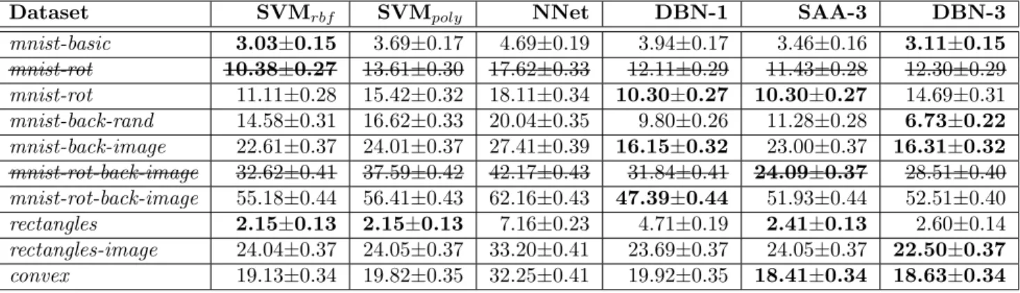
4.4.1 Benchmark Results . . . 70
4.4.2 Impact of Background Pixel Correlation . . . . 71
4.5 Conclusion and Future Work . . . 73
5 Presentation of the second article . . . 75
5.1 Article details . . . 75
5.2 Context . . . 75
5.3 Contributions . . . 76
5.4 Comments . . . 78
6 Why Does Unsupervised Pre-training Help Deep Learn-ing? . . . 81
6.1 Introduction . . . 81
xi
6.3 Unsupervised Pre-training Acts as a Regularizer . . . . 86
6.4 Previous Relevant Work . . . 88
6.4.1 Related Semi-Supervised Methods . . . 88
6.4.2 Early Stopping as a Form of Regularization . . 89
6.5 Experimental Setup and Methodology . . . 90
6.5.1 Models . . . 90
6.5.2 Deep Belief Networks . . . 91
6.5.3 Stacked Denoising Auto-Encoders . . . 92
6.5.4 Data Sets . . . 94
6.5.5 Setup . . . 94
6.6 The Effect of Unsupervised Pre-training . . . 96
6.6.1 Better Generalization . . . 96
6.6.2 Visualization of Features . . . 98
6.6.3 Visualization of Model Trajectories During Learn-ing . . . 99
6.6.4 Implications . . . 103
6.7 The Role of Unsupervised Pre-training . . . 103
6.7.1 Experiment 1: Does Pre-training Provide a Bet-ter Conditioning Process for Supervised Learning?104 6.7.2 Experiment 2: The Effect of Pre-training on Train-ing Error . . . 106
6.7.3 Experiment 3: The Influence of the Layer Size . 107 6.7.4 Experiment 4: Challenging the Optimization Hy-pothesis . . . 108
6.7.5 Experiment 5: Comparing pre-training to L1 and L2 regularization . . . 110
6.7.6 Summary of Findings: Experiments 1-5 . . . 110
6.8 The Online Learning Setting . . . 110
6.8.1 Experiment 6: Effect of Pre-training with Very Large Data Sets . . . 111
6.8.2 Experiment 7: The Effect of Example Ordering 113 6.8.3 Experiment 8: Pre-training only k layers . . . . 115
6.9 Discussion and Conclusions . . . 116
7 Presentation of the third article . . . 123
7.1 Article details . . . 123
7.2 Context . . . 123
7.3 Contributions . . . 124
7.4 Comments . . . 125
8 Understanding Representations in Deep Architectures 127 8.1 Introduction . . . 127
8.2 Previous work . . . 129
8.2.1 Linear combination of previous units . . . 129
8.2.2 Output unit sampling . . . 130
8.2.3 Optimal stimulus analysis for quadratic forms . 130 8.3 The models . . . 131
8.4 How to obtain filter-like representations for deep units 133 8.4.1 Sampling from a unit of a Deep Belief Network 133 8.4.2 Maximizing the activation . . . 133
8.4.3 Connections between methods . . . 135
8.4.4 First investigations into visualizing upper layer units . . . 136
8.5 Uncovering Invariance Manifolds . . . 142
8.5.1 Invariance Manifolds . . . 144
8.5.2 Results . . . 146
8.5.3 Measuring invariance . . . 148
8.6 Conclusions and Future Work . . . 149
9 Conclusion . . . 153
9.1 Main findings . . . 154
9.2 Speculative remarks . . . 155
List of Figures
1.1 Illustration of 4 different learning problems. . . 6
1.2 Illustration of 32-example dataset and a polynomial fit. 7 1.3 Dependence of polynomial fit on the hyper-parametres 11 2.1 The perceptron model. . . 20
2.2 Two learning problems, one solvable by the Perceptron and one that cannot be solved using a linear model. . . 20
2.3 Examples of activation functions . . . 21
2.4 A single-hidden-layer neural network . . . 22
2.5 A 2D binary classification problem . . . 25
2.6 Examples of shallow architectures . . . 31
2.7 A Restricted Boltzmann Machine . . . 36
2.8 Greedy layer-wise training of a Deep Belief Network . . 39
2.9 Greedy layer-wise training of a Stacked Auto-Associator 41 4.6 Samples from convex . . . 68
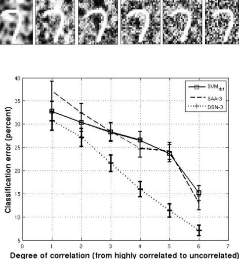
4.7 Samples with progressively less pixel correlation in the background. . . 72
4.8 Classification error on MNIST examples with progres-sively less pixel correlation in the background. . . 72
6.1 Effect of depth on performance for a model trained with-out unsupervised training and with unsupervised pre-training . . . 97
6.2 Histograms of test errors obtained on MNIST with or without pre-training . . . 97
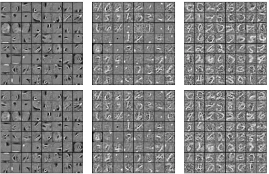
6.3 Visualization of filters learned by a DBN trained on In-finiteMNIST . . . 98
6.4 Visualization of filters learned by a network without pre-training, trained on InfiniteMNIST. . . 99
6.5 2D visualizations with tSNE of the functions represented by 50 networks with and 50 networks without pre-training101 6.6 2D visualization with ISOMAP of the functions repre-sented by 50 networks with and 50 networks without pre-training. . . 102
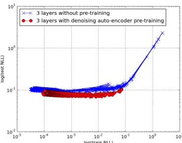
6.7 Training errors obtained on Shapeset when stepping in parameter space around a converged model in 7 random gradient directions. . . 103 6.8 Evolution without pre-training and with pre-training on
MNIST of the log of the test NLL plotted against the log of the train NLL as training proceeds . . . 106 6.9 Effect of layer size on the changes brought by
unsuper-vised pre-training . . . 108 6.10 For MNIST, a plot of the log(train NLL) vs. log(test NLL)
at each epoch of training. The top layer is constrained to 20 units. . . 109 6.11 Comparison between 1 and 3-layer networks trained on
InfiniteMNIST. Online classification error, computed as an average over a block of last 100,000 errors. . . 112 6.12 Error of 1-layer network with RBM pre-training and
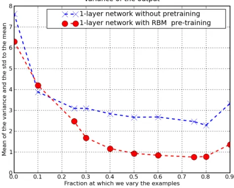
without, on the 10 million examples used for training it . . . 113 6.13 Variance of the output of a trained network with 1 layer.
The variance is computed as a function of the point at which we vary the training samples. . . 114 6.14 Testing the influence of selectively pre-training certain
layers on the train and test errors . . . 116 8.1 Activation maximization applied on MNIST . . . 138 8.2 Activation Maximization (AM) applied on Natural
Im-age Patches and Caltech Silhouettes . . . 141 8.3 Visualization of 6 units from the second hidden layer of
a DBN trained on MNIST and natural image patches. . 142 8.4 Visualization of 36 units from the second hidden layer of
a DBN trained on MNIST and 144 units from the second hidden layer of a DBN trained on natural image patches 143 8.5 Illustration of the invariance manifold tracing technique
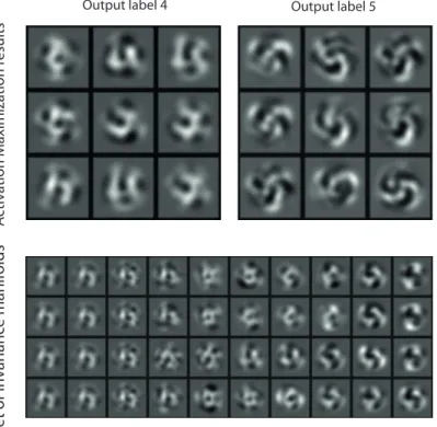
in 3D. . . 145 8.6 Output filter minima for the output units corresponding
to digits 4 and 5, as well as a set of invariance manifolds for each . . . 147 8.7 Measuring the invariance of the units from different layers.148
List of Tables
4.1 Results on the benchmark for problems with factors of variation . . . 71 6.1 Effect of various initialization strategies on 1 and 2-layer
Glossary
aa Auto-Associatoram Activation Maximization ann Artificial Neural Network cd Contrastive Divergence ce Cross-Entropy
crbm Conditional Restricted Boltzmann Machine dbm Deep Belief Network
dbm Deep Boltzmann Machine ebm Energy-Based Model
erm Empirical Risk Minimization
fpcd Fast Persistent Contrastive Divergence gp Gaussian Processes
hmm Hidden Markov Models
ica Independent Components Analysis kl Kullback-Leibler (divergence) lle Locally-Linear Embedding map Maximum a-posteriori mcmc Markov Chain Monte Carlo mdl Minimum Description Length ml Maximum Likelihood
mlp Multi-Layer Perceptron mrf Markov Random Field mse Mean Squared Error
nll Negative Log-Likelihood nlp Natural Language Processing nn Neural Network
pca Principal Components Analysis pcd Persistent Contrastive Divergence pdf Probability Distribution Function pl Pseudo-Likelihood
psd Predictive Sparse Decomposition rbf Radial Basis Function
rbm Restricted Boltzmann Machine saa Stacked Auto-Associator sae Stacked Auto-Encoder
sdae Stacked Denoising Auto-Encoder sesm Symmetric Encoding Sparse Machine sfa Slow Feature Analysis
sne Stochastic Neighbourhood Embedding srm Structural Risk Minimization
ssl Semi-Supervised Learning sv Support Vector
svm Support Vector Machine vc Vapnik-Chervonenkis
Acknowledgements
First and foremost, I extend my gratitude to Yoshua Bengio, the fearless leader of the LISA lab and my advisor who, at the onset of my PhD in 2006 warned me that he was embarking the whole lab on a long-term project—the study of deep architectures—which may fail (it did not). I thank him for his frankness, for his tireless and passionate attitude towards research, for the great advice, for making it possible to participate in this long-term project, and for being an inspiration throughout the MSc and PhD years at Universit´e de Montr´eal.
Aaron Courville deserves special recognition for being an amaz-ing person to work with. His pursuit of perfection—of results, of our writing, of our arguments—has considerably improved this thesis and the work contained within. I wish to thank the LISA lab members for being such a great gang, for the many great discussions we have had together, and for being great co-authors. Hugo Larochelle, James Bergstra, Nicolas Le Roux, Pierre-Antoine Manzagol, Douglas Eck, Guillaume Desjardins, Olivier Delalleau, Joseph Turian, Pascal Lam-blin, Pascal Vincent—it has been a pleasure working and sharing the same lab with you.
I also wish to acknowledge Samy Bengio and the people at Google Research with whom I collaborated during the past two years for pro-viding me with a great opportunity to test some of my ideas in a large-scale industrial setting.
Nicolas Chapados is responsible for the LATEX template that makes
this document so much more readable. Pierre-Antoine Manzagol and James Bergstra have provided me with useful feedback and suffered through reading the drafts of this document. The committee members have made this thesis better in a variety of ways, many thanks to them as well.
Stella, thank you for having been the perfect “partner in crime” during this whole PhD experience and for having stuck with me, against the odds. Finally, this thesis would not exist without the indefatigable support of my parents, Nadejda and Ion, whose optimism has never faded and who always believed in me.
1
Introduction
T
he field of Artificial Intelligence (AI) is at the intersection of a broad spectrum of disciplines, ranging from theoretical com-puter science, to statistics, many branches of mathematics, compu-tational neuroscience, robotics, cognitive psychology, and linguistics, among others. Its aims are to better understand intelligence, espe-cially human, and to eventually create such intelligence. The reasons for wanting to create it are varied, but the hope is that through such creation one can better understand the world around us, make scientific progress and introduce ways to benefit society at large.Since research in AI is so broad in its potential scope, there is a great variety of questions that researchers in this field can tackle: whether they relate to parallels between human (or animal intelligence) and the kind of intelligence that one can create with a computer program, or to the theoretical properties and limitations of algorithms that are commonly used in the literature.
Machine Learning (ML) is a subfield of AI, whose main subject is the study of learning from data. Just as AI is at the intersection of several disciplines, so is Machine Learning: it is admittedly difficult to draw a sharp line that differentiates the two, however research in ML tends to concentrate on the more computational aspects of artificial in-telligence, especially as they relate to learning from data. Whereas, for instance, a good portion of AI research is devoted to studying agents situated in a world, classical ML is typically concentrated on the mod-elling aspects of the same problem.
Both AI and ML research is heavily influenced by our perception and understanding of human and animal intelligence. Early advances in neuroscience, especially the computational aspects of it, have shaped the kind of algorithms and models that constituted the beginnings of ML research. The reason for that is simple: brains are the what makes human intelligent and they provide an example that we can take in-spiration from. By investigating them, we can not only advance the state of our knowledge regarding human intelligence, but we can hope to create new, intelligent models of the world.
In this thesis, we explore a class of machine learning algorithms that are inspired by our understanding of the neural connectivity and
organization of the brain, called deep architectures∗. The main goal of
this thesis is to advance the understanding of this class of learning algo-rithms. Sometimes our work took inspiration from our understanding of the human brain to better understand these algorithms, and other times it made it possible to frame the effects of these algorithms in terms of standard machine learning concepts. Ultimately, the contri-bution of this thesis is to ask and provide answers to questions that further our understanding of a large class of state-of-the-art models in Machine Learning and to make sure that these answers enable re-searchers in the field to improve on this state-of-the-art.
This thesis is structured as follows:
Chapter 1: defining intelligence, artificial intelligence, machine learn-ing, and the fundamental problem of machine learning: the prob-lem of generalization.
Chapter 2 : exploring attempts at to solving this generalization prob-lem, all the while paying attention to advances in our understand-ing of the short-comunderstand-ings of such solutions. In the same chapter, we describe deep architectures, the new class of algorithms that appear to possess qualities that make it possible to overcome said short-comings.
Chapters 3 and 4 : inquiry into these deep architectures, their prop-erties and their limitations. We begin by presenting our work on investigating how susceptible deep architectures are to certain variations of interesting learning problems, fundamentally and empirically.
Chapters 5 and 6 : we pin down certain ingredients from deep ar-chitectures into well-known Machine Learning concepts, and for-mulate a coherent hypothesis that gives us an idea as to why deep architectures can better solve the generalization problem.
Chapters 7 and 8 : we undertake the mission of building (mathe-matical) tools for qualitatively understanding deep architecture models.
Chapter 9 : provides a synthesis and discussion of our hypotheses, results, and tools.
∗. Throughout this thesis, the definition of deep architectures includes the struc-ture of the model as well as the algorithms used to learn in them.
1.1 Artificial Intelligence 3
1.1
Artificial Intelligence
There are various types and definitions of intelligence and intelli-gent behaviour. The type of intelligence that we will be referring to in this thesis is the kind found in humans and most animals. It is the kind of intelligence that allows us to infer meaningful abstractions when faced with an environment, be it through the transformation of the activations of photo-receptive cells of the retina into mental im-ages or through the transformation of air vibrations into useful mental representations such as words. This is definitely not the only manifes-tation of intelligence, as, in this discussion, we do not cover issues such as action, survival or reproduction, but limit ourselves to the passive forms of intelligence.
AI in general, and Machine Learning specifically, is concerned, among other things, with emulating intelligence. It is not necessary to copy the exact biological or physical mechanisms of humans in order to recre-ate their capabilities; indeed, one can treat humans as black boxes and instead build machines that behave like humans (in the input-output sense), but that do not necessarily function like humans. As long as the machine can produce the same kind of intelligence that we observe in humans (or even better one), we should be reasonably satisfied∗.
However, it would be wasteful to disregard the knowledge that we can obtain by investigating the mechanisms occurring in the human brain. This is because not only are humans in the unique position of pondering over their own intelligence, they are also the owners of brains that have evolved to intelligence unmatched by other animals on Earth. Human brains are thus successful examples of self-introspective intelli-gence, and therefore analyzing the principles behind the human brain (its organization, connectivity, evolution throughout lifetime and so forth) could help us greatly in understanding the nature of intelligence. It is very likely that there exists a number of ways of creating a system or agent that is intelligent—yet the mere existence of the brain suggests a prior over these possibilities, each of them being, in a vague sense, a computational view or model of how to learn and manipulate representations of the world. This means that we are better off at
∗. A famous argument against this idea is the Chinese Room Experiment. Searle (1999) argues that if he could convincingly simulate the behaviour of a native Chi-nese speaker, by following input/output instructions, he could conceivably pass the Turing test without actually understanding Chinese. In the context of the discus-sion on creating intelligence, this thesis will take a computational view on the theory of mind, arguing that we can view the brain as a mechanism for creating and ma-nipulating representations. In this respect, the quest to emulate these mechanisms is not as short-sighted as it might seem.
trying to search for a good model of the world in the vicinity of the model specified by the brain, than by starting in a completely random place.
It is probably this kind of thinking that led the first researchers of AI to the creation of the Perceptron (Rosenblatt, 1958), one of the first mathematical idealizations of the biological neuron (an “artificial neuron”). This was possible because of the advances in neuroscience, which analyzed the behaviour of biological neurons in the presence of an action potential. Nonlinear differentiable activation functions and an efficient way of training networks of one or more layers of such artificial neurons gave rise to a whole subfield of AI/ML—Artificial Neural Networks (ANN).
ANNs are neither truthful representations of the biological and chemical processes that happen in the brain, nor are they replacements for the brain (yet). They do provide however an example of how re-searchers can get inspiration from the brain and advance the state of the art in AI. As described in Chapter 2, ANN research is experiencing a revival, thanks to the discovery of useful and efficient ways of train-ing many layers of neurons. The techniques for traintrain-ing many layers of neurons, as well as the underlying models, are what we shall usually refer to as deep architectures throughout this thesis.
This work expands on this research by investigating the reasons why such techniques work. We are motivated by the fact that despite the recent advances in multilayer ANNs and despite the impressive experimental results, we lack a thorough understanding of what makes them work. Thus, we are looking for insights into these models. It is worth noting that we are not aiming for a better understanding of the brain as such; though we do not exclude the possibility of finding interesting parallels with results obtained by cognitive psychologists or computational neuroscientists, the research that is described in this thesis aims rather at a better understanding of the algorithms and models that we currently use.
1.2
Machine Learning
It is hard to imagine an intelligent system or agent that is not ca-pable of learning from its own experience. Therefore, we do not simply want a system that is able to come up with meaningful abstractions and representations of the world, given an environment. We want a system that is able to learn to come up with such abstractions and manipulate them, given a series of environments and time.
1.2 Machine Learning 5
We formalize certain basic notions of Machine Learning in the fol-lowing, so as to make the further discussions more precise. As men-tioned in the above, Machine Learning posits as a problem the creation of agents, systems, or algorithms that learn, either from data or from their environment. Data can in principle be anything that we can quantify in some way, but we shall usually deal with a set of vectors x called X , coming from an RDspace. A model of the data is a function
f , parametrized by a set of parameters θ, which maps elements of X to some space RT. We shall denote the output of f on X as the set
O = f(X ), with o ∈ O, while Y denotes the set associated with X , corresponding to the “true” (or optimal) model of the data. The task is then to find a procedure that would modify θ in such a way that o = f (x) would be as similar as possible to y, given x, with an empha-sis on generalizing to unseen vectors x in RD that are likely to come
from the same distribution as the elements of X . In other words, we are interested in finding that “true” model of the data, though this is an oversimplification (for presentation purposes), as in reality we operate on probability distributions and there does not necessarily exist a one-to-one mapping from X to Y; rather, we are interested in finding or approximating the joint distribution Px∈X ,y∈Y(x, y), with an emphasis
on obtaining the conditional P (y|x).
A learning algorithm specifies the sequence of steps that modifies the parameters of f in order to attain some objective L. Usually, L is some cost that penalizes the dissimilarity between o and y for some x. The learning algorithm is used to solve a specific instance of a learning problem. Depending on the type of y, we shall generally distinguish between the following types of problems:
classification : Y has finite cardinality. If the cardinality of Y = 2, we call this a binary classification problem. If the cardinality of Y > 2, we call it a multiclass classification problem. The unique members of Y are called labels and are given to the algorithm prior to learning.
regression : Y is an infinite and possibly unbounded subset of RT.
The values ofY are called targets and are given to the algorithm prior to learning.
clustering : Y is either a set of vectors from RD (which can be a
subset of X ) or a set of indices, neither given to the algorithm before or during training. The cardinality of Y is smaller than the cardinality of X .
embedding / projection : Y is a set of vectors in RT (where T can
to the algorithm prior to or during learning. The cardinality of Y is equal to the cardinality of X .
These four problems are illustrated in Figure 1.1. Note that we gloss over many variations in between these problems (and wholly different problems, such as reinforcement learning), since the examples shown in Figure 1.1 are the ones of particular interest for this thesis. Also note that classification and regression are examples of supervised learning problems, while clustering and embedding / projection are examples of unsupervised learning problems, the difference being the presence or the absence of Y during learning. Finally, this thesis will find special interest in problems that are at the intersection of supervised and unsu-pervised learning: these are called semi-suunsu-pervised learning problems.
� Figure 1.1. Illus-tration of 4 different learning problems. From left to right: a binary classification problem, a regression problem, clustering with cluster centers being part of the domain of X and an embedding /
projection problem
As described in the above, a learning algorithm is a functional that takes as inputsX , Y, L and a set of parameters θ and returns a modified set of these parameters θ∗, or, equivalently, a function f
θ∗ which can
then be applied to new input instances. This process is called training. Note that in case of clustering and embedding / projection, Y are not actually given to the learning algorithm. In those cases, the learning problem is to find a good way of representing X , rather than a way of approximating the relationship betweenX and Y. There is a variety of reasons for wanting a better representation, but the simplest one is that a good representation could, in principle, reveal interesting structure in X (as shown in Figure 1.1, where the projections of X separate better the examples from the two classes). Another reason for wanting a good representation is by viewing the problem of modelling X as that of density estimation, i.e., constructing a probability distribution function from the input instances given to us via X .
Finally, some notational aspects: the column vector corresponding to the D-dimensional input with index i in the dataset is xi. Its j th
component: xi
1.3 The Generalization Problem 7
predicted by some model is ˆyi. A column weight vector is θ and its jth
component is wj. A weight matrix is W and the element on the ith
row and jth column is Wij.
1.3
The Generalization Problem
Consider a simple example (in Figure 1.2), which is a 1-dimensional 32-example dataset (blue crosses), generated by yi = sin(xi)+N (0, 0.25) where N (0, 0.25) is a univariate Normal noise with mean zero and stan-dard deviation of 0.25. The learning algorithm does not see the gener-ating function, but just the (xi, yi) pairs. This is a supervised learning problem, where the algorithm has to perform regression. The subset of the input setX × Y that we shall use for getting θ∗ is called a training
set, denoted by Dtrain. In our 32-example case, this is represented by
half of the examples (randomly chosen).
� Figure 1.2. Illustration of a 1-dimensional 32-example dataset (blue crosses), generated by yi= sin(xi) + N (0, 0.25) where N (0, 0.25) is a
univariate Normal with mean zero and standard deviation of 0.25,
x∈ [−3; 3], and i = 1, . . . , 32. The green curve corresponds to a polynomial of degree 5, found by minimizing the Mean Squared Error (MSE).
This serves as the prototypical scenario for the discussion on the fact that solving the learning algorithm—finding a function or its pa-rameters that minimizes L given the training data—is not an easy en-deavour. First, there is an infinite number of functions that can provide
an error-free mapping from the given inputs to the given outputs∗. We
are thus presented with a few important questions: how can one even enumerate or search through these functions? Does it matter which function we ultimately choose? And if yes, is there a criterion that we can use to choose from these functions?
1.3.1
Training and Empirical Risk Minimization
In the most general case possible, without making any further as-sumptions, we cannot search through all the possible function mappings in finite time. So we need to restrict ourselves to a class of functions which we can either enumerate or search through easily. In this partic-ular case, we could restrict ourselves to the model class of polynomials, meaning that we will seek functions of the type
fk(x, θ) = θ0+ k
�
j=1
θjxj
where xj is x to the jth power and where we will denote θ = θ
0, . . . , θk.
In general, models of the data can either be parametric or non-parametric. A parametric model class has a fixed capacity for any size of the training set, whereas a nonparametric model’s capacity generally grows with the size of the training set. The capacity of a model class is roughly the cardinality of the set of functions represented by it. This is just one of the few definitions for this concept; intuitively, it states that if a model class has greater capacity it can model more (and more complex) functions, since there are, in principle, more functions to choose or search from. The polynomial model that we investigate corresponds to a parametric model of the data. This is because, in our example, a polynomial of degree k is a class of functions, as it represents all functions which have the form of a polynomial of degree k, meaning the weight vectors of all polynomials of degree k; the number of such functions† is fixed during training and does not grow with the size of the data.
Assuming that we can efficiently find the polynomial of degree k that “fits” the data best, then the problem should be easily solved. Unfortunately, there are certain steps in this procedure which need to
∗. Moreover, it is not at all clear that we want an error-free mapping, since we, as designers of the learning problem generated the data with noise. However, the learning algorithm does not have, generally speaking, access to such information
†. The number of such functions is infinite, but we can make statements that polynomials of degree k are a subset of polynomials of degree k + 1 and hence the former class of functions has fewer functions.
1.3 The Generalization Problem 9
be further refined and which play a major role in the kind of model we will get at the end. First, we need to define what we mean by “fit”: how do we measure whether a certain function fits the data? We can take a Mean-Squared Error (MSE) approach and define the degree of fit between the predictions ˆyi = f
k(xi, θ) of this function and the outputs
as E(k, θ, Dtrain) = N�train i=1 � ˆ yi− yi�2
where xi is the ith 1-dimensional input example, yi is the
correspond-ing output, k is the degree of the polynomial, and θ the parameter vector corresponding to the specific polynomial that we are analyzing. E(k, θ, Dtrain) is what we called a loss functional in Section 1.2.
The principle of defining a function class and choosing a function from this set, which minimizes a given training error is called Empiri-cal Risk Minimization (ERM) (Vapnik and Chervonenkis, 1971). What one typically wants to minimize is the true risk, meaning the loss func-tional evaluated over the entire distribution p(x, y), but generally we cannot do that and have to make do with the finite training set that is at our disposal.
The choice of Mean-Squared Error might seem arbitrary and this is true in the absence of other information. It turns out that it is a natural option when solving a regression problem. Assume we have a loss L(y, f (x)) and a distribution p(x, y) over which we want to compute this loss. The expected loss is then
Ex,y[L] =
� �
L(y, f (x))p(x, y)dxdy
If the chosen loss is (y− f(x))2, then we can differentiate E
x,y[L] with
respect to f (x). When setting to zero, the function f (x) that minimizes this expected loss becomes Ey[y|x], which is the conditional expectation
of y given x, also called the regression function.
In our particular case, for a given k, the fact that fk(x, θ) is a
linear function in θ and that MSE is a quadratic function of θ implies that we can efficiently find the θ that minimizes E(k, θ, Dtrain) (this is
equivalent to performing least-squares regression with a simple linear model). The solution to this optimization problem is unique, given k and Dtrain; let us denote it by θ∗. Figure 1.4(a) shows E(k, θ∗, Dtrain),
the training error, for each k. As one would expect, the larger k is, the better the fit and when k ≥ Ntrain − 1, the MSE will necessarily be
1.3.2
Validation and Structural Risk Minimization
One of the standard procedures for verifying the quality of a model validation: it is the computation of a loss functionalLvalid (which couldbe different from L) on some (statistically independent from Dtrain)
subset of X × Y called the validation set Dvalid. Validation is needed
for choosing between the hyperparameters of a learning algorithm— those parameters which are not directly optimized during training, but which still influence the quality of the parameters θ∗ that are found by applying the Empirical Risk Minimization principle. A model class indexed by some hyperparameters λ is a subset of functions from X to Y whose parameters are θλ. The tuple (λ, θλ∗) that minimizes Lvalid is
the one we should choose as our model.
In our example, the only hyper-parameter is k. cannot guide our-selves by E(k, θ∗, Dtrain) for choosing an optimal k. The validation
principle requires us to split the data available into a training set, which we did by defining Dtrain as a random half of the data, and a
validation set Dvalid, the other random half in our example. Then, one
uses the validation loss functional on Dvalid to make decisions about
hyper-parameters. In our example, the validation loss functional that we will define is going to be MSE again.
In Figure 1.4(a) we see a curve that is common in many machine learning experiments: there seems to be a k∗ (at around k = 5) for
which the error on the validation set (the validation error ) is lowest. Any model with k < k∗ seems to underfit the data, meaning that it
does not have enough capacity (large enough number of functions from which to choose), whereas any model with k > k∗ seems to overfit the data, meaning it likely has too much capacity.
To get an unbiased estimate of the performance of the model rep-resented by k = k∗, we would need to test the best model on a test set Dtest (independent of Dtrain and Dvalid) using some loss functional,
which is normally Lvalid. This unbiased estimate of the performance of
the model is also called the generalization error and choosing a model class which allows to us efficiently obtain the lowest generalization er-ror for a given learning problem is the central problem in Machine Learning.
While the method by which we chose k—the one that minimizes the validation error—is popular and intuitively sound, it is certainly not the only way in which we could proceed. For example, the principle of “Occam’s Razor”, which says that one should choose the simplest model that explains the data Blumer et al. (1987), has also been inves-tigated. More generally, the procedure for giving preference to certain configurations of the parameters at the expense of others is called
reg-1.3 The Generalization Problem 11
ularization. Both parametric and nonparametric model classes can be regularized : this means that one can impose constraints on the type and richness of functions that can be used or learned, i.e. we can con-strain the capacity of the model class. Regularization typically acts as a trade-off mechanism between fitting the training data and having a good model for previously unseen examples.
Getting back to our example, let us take the class of functions that is represented by the polynomials of degree k∗. A specific instance from this class is in Figure 1.2. One way of constraining the parameters of this function class is to minimize it by modifying the loss function such that E(k, λ, θ, Dtrain) = N�train i=1 � fk(xi, θ)− yi �2 + λ||θ||2
Minimizing this loss function is otherwise known as ridge regression (Ho-erl and Kennard, 1970).
The principle of adding a constraint to the process of Empirical Risk Minimization so as to favour certain functions in a given class is called Structural Risk Minimization (SRM) (Vapnik, 1982). Assuming one can measure the complexity of a given model or model class (norm of parameters, degree of polynomial, etc.), the SRM principle is a general way of choosing among models, by simply selecting the one whose sum of the empirical risk and complexity level is minimal. In this sense, SRM is a trade-off between the data fit and the complexity of a given model and is a principled way of performing regularization.
� Figure 1.3. MSE as a function of the degree of the polynomial and of λ, the regularization parameter (for k = 5, the degree that
minimizes the error on the validation set)
(a) Degree of the polynomial (b) λ, the regularization parameter
In our case, the λ||θ||2 regularizer introduces a penalty proportional
to the square of the magnitude of each weight, which in the particular case of polynomials, will encourage functions with small parameter val-ues, i.e., polynomials with small coefficients. Figure 1.4(b) shows the
value of the training and validation errors as a function of λ, the regu-larization value. Note that this is not, in the strictest sense, the appli-cation of the Structural Risk Minimization principle. SRM would make us choose λ to minimize E(k, λ, θ, Dtrain) + C(k, λ, θ), where C(k, λ, θ)
is a measure of complexity of the model specified by k, θ and λ (and not the value of k, θ and λ). It is unfortunately not obvious to define such a complexity measure; fortunately, simply evaluating E(k, λ, θ, Dvalid)
is a reasonable and very popular alternative. As with k, λ trades off simplicity with data fit and, as before, there seems to exist a value of λ that minimizes such a trade-off; like before, we can interpret any model with λ smaller or larger than this optimal value as underfitting or overfitting, respectively.
Even after performing regularized polynomial fitting on our data, the result in Figure 1.2 should tell us that our job of finding a class of functions that generalizes well is far from finished. While the polyno-mial of degree k∗ = 5 found with MSE is able to model the underlying function well within the data bounds, it is clearly mismatched with the target function, as it does not extrapolate well. This mismatch is a consequence of our choice to restrict ourselves to polynomials in our search: no polynomial will be really able to model a sinusoid, and we are bound to have numerical and stability issues if we have to re-sort to fitting polynomials of very high degree. This is an important lesson as it shows that even when a model is theoretically guaranteed to be able to represent any function∗, it might not be at all efficient
and one might run into the trouble of the target function simply being mismatched with the class of functions considered during learning.
1.3.3
The Bayesian approach
So far we have taken a function approximation approach to mod-elling: we have defined the result of learning a single θ∗, given to us by
a combination of a learning objective functional and a model selection scheme. This θ∗ represents the set of parameters or function that we
believe, based on measures such as the lowest validation error, would best generalize to unseen data.
The basic idea of the Bayesian approach is that within a given class of functions (specified, say, by a combination of hyper-parameters), several θ could seem as appropriate choices: when predicting the out-put for a previously unseen xnew, one has to somehow integrate or
average over all of these choices, weighing them in a principled
man-∗. It is easy to convince oneself that a polynomial can approximate any reason-ably smooth function of the input, given sufficient data and a large enough degree.
1.3 The Generalization Problem 13
ner. Formally, if f (x, θ) is how we parametrize our function class (e.g., polynomials of a certain degree), then we should be making decisions by
Eθ(y|xnew, Dtrain) =
�
f (xnew, θ)P (θ|Dtrain)dθ
where we weigh each prediction by P (θ|Dtrain), the posterior
distri-bution of the parameters given the training data. Unfortunately, this integral is intractable for a lot of functions that are of interest to us and most often one has to resort to approximations, such as in the procedure for computing, approximating or sampling from P (θ|Dtrain).
To obtain P (θ|Dtrain) one uses the Bayes theorem:
P (θ|Dtrain) = P (Dtrain|θ)P (θ)/P (Dtrain)
Central to the Bayesian approach is the notion of a prior over the pa-rameters: P (θ) encodes our prior belief in the distribution of θ without having seen any training data. P (Dtrain|θ) is the likelihood of the data
given a setting of the parameters: we shall see in the following that the analysis of this distribution is of interest to us.
One of the more useful approximations that one could make during the process of applying the principles of Bayesian inference is the MAP (Maximum A-Posteriori) approach, which is the principle of choosing the θ that maximizes the posterior
θM AP = arg max
θ P (θ|Dtrain) = arg maxθ P (Dtrain|θ)P (θ)
The intuition is that the mode of the posterior distribution is a good point estimate of the entire distribution. For certain simple distribu-tions (such as the multivariate Gaussian) the mode is indeed a repre-sentative point estimate∗.
Depending on the shape of the prior or the likelihood, computing θM AP can be difficult or intractable, because the posterior distribution
could be multi-modal. Often the solution is to use the principle of Max-imum Likelihood, which states that one should choose θ to maximize
θM L = arg max
θ P (Dtrain|θ)
which is the likelihood of the data given the parameters. There are connections between the ERM/SRM and ML/MAP principles, respec-tively. To reveal these connections within our polynomial modelling framework, we have to cast the problem in a probabilistic setting, since
∗. Naturally, the MAP estimate may be a poor approximation for a multi-modal posterior distribution.
no mathematical object that we looked at so far in our discussion on polynomial fitting defines a probability of any sorts. If we take our example of fitting a polynomial to the data, we can define a distribu-tion that represents the uncertainly that we have in our predicdistribu-tion for a given fk(x, θ):
p(y|x, θ) = N(y|fk(x, θ), σ2)
where fk(x, θ) is the polynomial as defined before and N (y|fk(x, θ), σ2)
is a Gaussian distribution centered at fk(x, θ) with a standard deviation
of σ.
Assuming that our data is i.i.d. and drawn from this distribution, for a given training set (xi, yi), where i = 1, . . . , N
train, the conditional
likelihood of the data given the parameters is
p(Dtrain|θ) = N�train
i=1
N (yi|fk(xi, θ), σ2)
Maximizing p(Dtrain|θ) implies taking the log, differentiating wrt. to θ
and setting to zero: one can then see that maximizing the likelihood is equivalent to minimizing the Mean Squared Error on the training set. Thus, when assuming an Gaussian model for our probabilistic predictions, the ML solution—call it θM L—is equivalent to the MSE
method we used when applying the ERM principle before.
Likewise, if we incorporate a prior P (θ) = N (0, λI) into our pre-dictions, then maximizing the posterior P (θ|Dtrain)∝ P (Dtrain|θ)P (θ)
with respect to θ means finding the θ that minimizes
N�train i=1 � fk(xi, θ)− yi �2 + λ||θ||2
Therefore, we see that the squared penalty we used to regularize when applying the SRM principle is equivalent to introducing an isotropic Gaussian prior on the weights (with a standard deviation that is equiv-alent to λ in our model) and finding the MAP solution—θM AP—to the
problem.
With either θM L or θM AP we can make predictions for previously
unseen inputs by simply evaluating p(y|x, θM L) or p(y|x, θM AP) for a
given x. A full Bayesian treatment, as mentioned in the above, requires us to not simply come up with a point estimate of θ, but marginalize over the entire posterior distribution when P (θ|Dtrain) when making
decisions. Thus, we would like to be able to calculate distributions of the form
p(y|x, Dtrain) =
�
1.4 The Inevitability of Inductive Bias in Machine Learning 15
For the distributions that we considered so far (uni and multi-variate Gaussians) this can be done analytically, since computing the integrals is a matter of convolving two Gaussians. Thus, p(y|x, Dtrain) is a
Gaus-sian itself, whose mean and standard deviation are functions of x, the unseen input.
Often, one can use complicated multi-modal prior distributions if one makes approximations, either in the inference or in the learning process, or both. However, taking the Bayesian approach to modelling and inferring point estimates or posterior parameter distributions is al-most always a trade-off between the mathematical convenience of hav-ing tractable distributions (i.e., over which one can tractably evaluate integrals or sums) and having powerful models of the data.
1.4
The Inevitability of Inductive Bias in
Machine Learning
What transpires from the discussion so far is that there is a mul-titude of choices that one makes before arriving at a model that is satisfactory:
– The class of functions to consider for modelling: polynomial, per-ceptrons, artificial neural networks, etc.
– The general principle for optimization or inference in this class of functions: maximum likelihood or ERM, MAP or SRM, fully Bayesian, etc.
– Model choice or selection procedure: the choice of the loss func-tional, including how to split the available data intro training, validation and test sets.
– Model constraints: how to regularize the model such that cer-tain parameter configurations are more preferred than others or, equivalently, which prior distribution to use in a Bayesian frame-work.
One might question whether automatic machine learning is possible without us making so many choices. It is instructive to think of the functions that we are searching through as hypotheses that explain our data. The choices that we make at each stage during learning either exclude certain hypotheses from our search altogether∗ or change the
likelihood with which our search procedure will consider them†.
∗. For instance, the choice of considering only polynomials of order k excludes all the other hypotheses
Every time we make a choice of this type, we are biasing the opti-mization or search through the hypothesis space. A fundamental result in Machine Learning is that bias-free learning is not possible (Mitchell, 1990), for there is always generally an infinite number of hypotheses that explain the data equally well. Equivalently, it is not possible to generalize without having an inductive bias, which allows us to define a preference for certain hypotheses vs. others; without an inductive bias, we will not be able to have a meaningful way of learning from data.
Another fundamental result in optimization and machine learn-ing, the No-Free Lunch theorem (Wolpert, 1996), states that for every learning algorithm (that generates hypotheses from data) there always exists a distribution of examples on which this model will do badly. In other words, no completely general-purpose learning algorithm can exist, therefore every learning algorithm must contain restrictions— implicit or explicit biases—on the class of functions that it can learn or represent.
Biases can come in different flavours, but generally we can dis-tinguish between representational and procedural biases (Gordon and Desjardins, 1995). A representational inductive bias is one that makes the hypothesis space incapable of modelling all possible hypotheses that are compatible with the training data, because of the limitations on the kind of hypotheses that can be constructed. A representational bias can be strong if the hypothesis space that corresponds to it is small; con-versely, the bias is weak if the hypothesis space is large (Utgoff, 1986). Analytically, one can measure the strength of a bias via the Vapnik-Chervonenkis (VC) dimension (Vapnik and Vapnik-Chervonenkis, 1971), which is an indirect measure of the capacity of the model∗. Finally, one can also measure the correctness (Utgoff, 1986) of a bias: namely, whether the hypothesis space defined by it contains the “correct” hypothesis or not.
A procedural bias makes the search or inference procedure itself bi-ased towards certain hypotheses. Maximum likelihood, Occam’s razor, MAP are all example of such procedural biases. Another popular way of encoding a preference for a given hypothesis is the principle of Min-imum Description Length (MDL) (Solomonoff, 1964; Rissanen, 1983), which specifies that preference should be given to hypotheses that al-lows for the best (or shortest) encoding of the data†. In one way or another, inductive biases are present in all machine learning algorithms for otherwise, as Mitchell (1990) put it “an unbiased learning system’s
∗. Defined by the cardinality of the set of hypotheses that this model can rep-resent or, more precisely, by the largest set of points that the model can shatter.
1.4 The Inevitability of Inductive Bias in Machine Learning 17
ability to classify new instances is no better than if it simply stored all the training instances and performed a lookup when asked to classify a subsequent instance”.
Since inductive bias is always present, we have a certain freedom to choose when designing the process of learning. Frequently, the choice is made towards a weak representational bias, therefore making sure that the hypothesis space considered is the most general possible class of functions over which we can define a preference; this is to ensure that our representational bias is correct, i.e., does not exclude the target hypothesis. But we should always be aware that our choice must be made such that interesting and complicated functions or hypotheses are actually learnable (in finite time), using standard algorithms applied on functionals that take this model class as inputs. This is true even in the context of models that are in principle able to model arbitrary input-output mappings∗: inductive bias is still an important tool, since not all
these models actually allow for interesting and complicated functions to be learned with finite amounts of data, or time, or simply a number of examples which is not exponential in the number of intrinsic variations in the data.
Modern Machine Learning problems have a few properties which make the process of training, or approximating the relationship be-tween X and Y and coming up with hypotheses that generalize well, quite difficult. Any technique for solving the generalization problem must scale well in the number of dimensions of the inputs x and the number of examples considered. Typical ML problems have complex input variations and noise, either in the labelling process or in the data itself, and simple approaches that rely on enumerating the data vari-ations could be extremely inefficient. The generalization problem is even more acute in such a setting, because, as we shall see in Chapter 2, some of the typical representational and procedural inductive biases and assumptions—related to the classes of functions, or the regularity in the input data—simply do not hold for realistic machine learning datasets and problems.
In this thesis, we study the deep architectures. Any instance of these models (and associated learning procedures) is a parametric model of the data, but we are free to choose the capacity of the model based on validation data; this makes the model family non-parametric as well. The combination of these properties is desirable, for it allows us to tune the size of the hypothesis space in a principled manner. One is also able to leverage unsupervised data during the training process, a step which
∗. These mappings typically have reasonable properties, such as functions with compact support and having certain continuity properties.
we show crucial in Chapter 6. Their hierarchical structure makes the models compact and highly nonlinear representations of the data and its variations and, empirically, they show great promise in a variety of application domains. Thus, deep architectures provide an interesting inductive bias and this thesis is an exploration of the consequences that this inductive bias has on the hypotheses that we can learn from data.
2
Previous work: from
perceptrons to deep
architectures
I
n this Chapter we review some important developments in Ma-chine Learning, with an emphasis on Artificial Neural Networks. By any measure, it is not meant to be a comprehensive overview of the history of the field, but rather a background on the work that shaped the ideas presented in the later parts; there is also more emphasis on the state of the art in the field.2.1
Perceptrons, neural networks and
backpropagation
As previously mentioned, one of the first brain-inspired AI mod-els was the Perceptron by Rosenblatt (1958), presented in Figure 2.1. Sidestepping the complications that arise with modelling real, biological neurons, where differential equations govern their behavior, perceptrons are artificial neurons whose behavior is a highly simplified version of the real neurons. The basic idea is that a neuron receives inputs from other neurons (the connections between them corresponding to den-drites in a biological neuron), sums these inputs and passes the sum through an activation function. The output of the activation function is then passed to the next neuron (corresponds to an axon). As shown in Figure 2.2 (left), the activation function of a perceptron is similar to the one used in biological neurons—a step function (also called the Heaviside function, see Figure 2.3). It corresponds to the neuron “fir-ing” (or being “on”) when the weighted input sums to a value above a threshold.
The perceptron algorithm came with a learning rule for modifying its weights to attain a classification objective. Importantly, under cer-tain conditions, this rule will converge to a set of weights that gives zero errors. One such condition is the linear separability of the input examples, as illustrated in Figure 2.2 (left): linear separability means that there exists a hyperplane in the D-dimensional space of x that can separate (error-free) the input examples. If such a hyperplane exists,
� Figure 2.1. The perceptron: a mathematical idealization of the biological neuron.
then the perceptron rule will converge to it; otherwise, there is no guar-antee of that happening. A finding with significant impact at that time was that for a variety of problems, linear separability does not apply. Minsky and Papert (1969) have demonstrated that perceptrons are not able to solve seemingly simple problems such as the XOR-problem∗,
which is not linearly separable (see Figure 2.2).
� Figure 2.2. Left: a binary classification problem where there exists a separating hyperplane. Right: the XOR problem, where no separating hyperplane exists and where the perceptron algorithm will not converge
This work was influential enough to slow down research into ANNs for a period of 15 years. Refinements and improvements to the basic linear threshold model were certainly being done, and Widrow and Lehr (1990) present a comprehensive examination of the history of single-layer networks in that period of time; however, a breakthrough was needed in order to overcome the issue of linear separability.
For this breakthrough to occur, two important things had to hap-pen:
– The realization that differentiable nonlinear activations allowed much easier numerical optimization.
– An efficient way of training of networks containing such elements.
∗. The inputs are all the possible combinations for two bits and the outputs are the respective application of the XOR function on these inputs
2.1 Perceptrons, neural networks and backpropagation 21
The backpropagation algorithm, discovered independently by several researchers in a span of 12 years (Werbos, 1974; Parker, 1985; LeCun, 1986; Rumelhart et al., 1986) provided just that. First, the Heaviside step function was replaced by a sigmoid as the activation function. The latter is a family of functions, having roughly an “S”-shape, closely related to the damped nonlinear response that a biological neuron has∗. Typical examples from this family are the logistic sigmoid
sigm(x) = 1
1 + exp(−x) and the hyperbolic tangent
tanh(x) = exp(x)− exp(−x) exp(x) + exp(−x) . Both are illustrated in Figure 2.3.
� Figure 2.3. Illus-tration of activation functions: the step function, the sigmoid, and the hyperbolic tangent
Replacing either of these formulas as the transfer function of a per-ceptron does not make a significant difference, since the resulting model is a logistic regression model, which suffers from the same issue of linear separability. The key insight is shown in Figure 2.4: one can now build layers of such units† and the more sigmoidal units we add to a layer,
∗. It can also be viewed it as a “soft” step function
†. One could have built multiple layers of perceptrons, too, in a similar fashion. However, the discontinuous and non-differentiable activation function did not lend itself easily to a learning algorithm such as backpropagation, presented below.
the more nonlinear the relationship between the input and the output becomes. This is because the output is now computed as a weighted sum of outputs of these units. Sigmoidal units are then called “hidden units” and the layers containing them are “hidden layers”.
� Figure 2.4. A single-hidden-layer neural network that takes a D dimensional vector as input, nonlinearly projects it to a N -dimensional hidden unit space and retrieves an output by a weighted
combination of the hidden units followed by the application of an output transfer function
Formally, a single-output, single-hidden-layer neural network, as represented in Figure 2.4 computes the following mathematical func-tion:
ˆ
y = f (v�sigm (W x)) (2.1) where W is the input-to-hidden weight matrix, v are the hidden-to-output weights∗, x is the input and f () is the output transfer function:
it transfers the output of the network into the domain that is problem-specific (the domain of y, the label/target corresponding to its estimate computed by the network, ˆy). This formalization can be easily extended to an arbitrary number of hidden units, hidden layers and outputs.
Why is a differentiable activation function important? The above-mentioned researchers had another key insight: the output of equation 2.1 is differentiable with respect to all of its parameters. Given a differ-entiable objective function, E(ˆy, y, x) that can compute some measure of error between the prediction of the network ˆy and the true y cor-responding to some x, we can now compute the gradient of the error with respect to the parameters of the network.
For each of the problems described in Section 1.2 one can find suit-able differentisuit-able objective functions, as there is a natural pairing
be-∗. Typically, a neural network implementation contains a bias vector/term as well, which can be seen as a weight that does not depend on the input
2.1 Perceptrons, neural networks and backpropagation 23
tween the output transfer function, the error used and the problem to be solved:
– In the case of regression, the squared error is the most popular choice: E(ˆy, y, x) = (ˆy− y)2 and the output transfer function is
simply the identity.
– With binary classification, the output transfer function is usually a logistic sigmoid and ˆy can be interpreted as the probability p(y = 1|x); the objective function is then the cross-entropy E(ˆy, y, x) = −y log ˆy− (1 − y) log(1 − ˆy), assuming y ∈ {0, 1}, which is simply − log p(y|x), i.e. the negative log-likelihood.
– For multiclass classification problems, the so-called softmax is the natural choice for the output transfer function as it projects the output of the network onto a set of probabilities that sum to one, corresponding to p(yk|x), where k is an index into the classes:
p(yk|x) = softmax(tk) =
exp(tk)
�
jexp(tj)
where t is a vector of outputs of the network. By transform-ing y into a one-hot vector∗ we can use the negative likelihood − log p(y|x), too.
– For finding an embedding of the input x one view the network as encoding the input into the output domain. The process of decoding will transform the output of the network into the same domain as x and use either the squared error or the cross-entropy to minimize the disparity between the original input and the de-coded one. The activations of the hidden layer could then act as the embedding of the data, meaning that they are a new (and hopefully better) representation for the input.
The gradient gives the direction of the steepest ascent in the error space. Therefore, by moving in the direction opposite of it, we can perform gradient descent and modify the parameters of the network so as to reach a (local) minimum in the error space. Computing the gradient efficiently was the other ingredient to the success of neural networks after Rumelhart et al. (1986)’s publication. The main idea is that that we can recursively compute the gradient with respect to the outputs of each unit, once the gradients for the layer above are known; hence the name backpropagation.
This recursive structure gives rise to an efficient algorithm for com-puting the required gradients since a complete backpropagation pass takes only O(k) (with k being the number of weights). This was a
∗. Corresponding to a vector that is all zero except at position k where k is the class number