Topologie digitale dans un espace localement fini
par
Jeremy GODIN
memoire presente au Departement de mathematiques
en vue de I'obtention du grade de maitre es sciences (M.Sc.)
FACULTE DES SCIENCES
UNIVERSITE DE SHERBROOKE
1*1
Library and Archives Canada Published Heritage Branch 395 Wellington Street Ottawa ON K1A 0N4 Canada Bibliotheque et Archives Canada Direction du Patrimoine de I'edition 395, rue Wellington OttawaONK1A0N4 CanadaYour file Votre reference ISBN: 978-0-494-53166-2 Our file Notre reference ISBN: 978-0-494-53166-2
NOTICE: AVIS:
The author has granted a
non-exclusive license allowing Library and Archives Canada to reproduce, publish, archive, preserve, conserve, communicate to the public by
telecommunication or on the Internet, loan, distribute and sell theses
worldwide, for commercial or non-commercial purposes, in microform, paper, electronic and/or any other formats.
L'auteur a accorde une licence non exclusive permettant a la Bibliotheque et Archives Canada de reproduire, publier, archiver, sauvegarder, conserver, transmettre au public par telecommunication ou par I'lnternet, prefer, distribuer et vendre des theses partout dans le monde, a des fins commerciales ou autres, sur support microforme, papier, electronique et/ou autres formats.
The author retains copyright ownership and moral rights in this thesis. Neither the thesis nor substantial extracts from it may be printed or otherwise reproduced without the author's permission.
L'auteur conserve la propriete du droit d'auteur et des droits moraux qui protege cette these. Ni la these ni des extraits substantiels de celle-ci ne doivent etre imprimes ou autrement
reproduits sans son autorisation.
In compliance with the Canadian Privacy Act some supporting forms may have been removed from this thesis.
Conformement a la loi canadienne sur la protection de la vie privee, quelques
formulaires secondaires ont ete enleves de cette these.
While these forms may be included in the document page count, their removal does not represent any loss of content from the thesis.
Bien que ces formulaires aient inclus dans la pagination, il n'y aura aucun contenu manquant.
1*1
Canada
Le 5 aout 2009
lejury a accepte le memoir e de M. Jeremy Godin dans sa version finale.
Membres dujury
M. Madjid Allili
Directeur
- Bishop's University
M. Tomasz Kaczynski
Codirecteur
Departement de mathematiques
Mme Virginie Charette
Membre
Departement de mathematiques
M. Jean-Marc Belley
President-rapporteur
Departement de mathematiques
SUMMARY
Dans ce memoire, nous presentons d'abord une introduction a la theorie classique de la topologie digitale en utilisant une approche de "graphe d'adjacence". Les concepts de cette theorie sont examines en detail et ensuite, rtous discutons des desavantages inherents a cette approche, dus essentiellement au manque de rigueur axiomatique dans son elaboration.
Par la suite, nous etudions une nouvelle approche a la theorie de topologie digitale telle que developpee par V. Kovalevsky. Cette theorie, basee sur une approche axiomatique, permet de contourner la plupart des problemes rencontres dans la theorie classique. Elle presente des axiomes pour bien definir une topologie digitale. Apres avoir presente les axiomes, nous construisons un contre exemple qui demontre une inconsistance dans l'approche de Kovalevsky. Afin de pallier a cette difficulte, un nouvel axiome est rajoute a cet efFet.
Au lieu de se consacrer a 1' etude des complexes cellulaires abstraits, nous faisons appel a la theorie des CW-complexes, telle que developpee par J.H.C Whitehead, et aux com-plexes cubiques, tels que formalises par T. Kaczynski et al. pour etablir des liens entre la toplogie digitale axiomatique et la topologie algebrique dont le formalisme puissant per-met d'elargir les champs d'application de la topologie digitale. Finalement des exemples concrets sont donnes pour demontrer l'utilite de cette theorie pour l'analyse d'images
ACKNOWLEDGEMENTS
First and foremost I would like to thank my advisers Madjid Allili and Tomasz Kaczynski for giving me the opportunity to study with them. Their guidance and patience over the past three years made this work possible. I would equally like to acknowledge the support given to me by my friends and colleagues over the past years, notably Stephen McManus, Jennifer Tremblay-Mercier, Marc Ethier, Bernard Wagneur, Audrey Samson, and many others I'm sure I omit. Finally, I would like to thank my family who I know I can always count on.
Jeremy Godin Sherbrooke, October 2008
TABLE OF CONTENTS
SUMMARY Hi
ACKNOWLEDGEMENTS v
TABLE OF CONTENTS vi
LISTE DES FIGURES viii
INTRODUCTION 1
CHAPTER 1 — Classical Digital Topology 4 1.1 Adjacency Relations and Connectedness 4
1.2 Digital Pictures 10
1.3 On Simple Closed Paths, Holes, Borders, and Cavities 13
1.4 Euler Characteristics and Continuous Analogs 28
2.1 Inconsistencies in the Classical Approach 34
2.2 The Axioms of Digital Topology 36
2.3 Relationship to Classical Topology 40
2.4 Properties of Axiomatic Locally Finite Spaces 42
CHAPTER 3 — Preliminaries 52 3.1 CW and Cubical Complexes 52
3.2 Cubical Complexes 56
3.3 Homology 57
3.3.1 Elementary Collapse . . 67
CHAPTER 4 — Applications of Axiomatic Digital Topology 70
4.1 Digital Images in AC complexes 70
4.1.1 Data Structures 71
4.2 Practical Algorithms for Axiomatic Digital Topology Using the Cell
Com-plex Structure 73 4.2.1 Boundary Tracing 74 4.2.2 Filling of Interiors 76 4.2.3 Component Labeling 80 4.2.4 Skeletons of a Set in 2D 82 CONCLUSION 85
LIST OF FIGURES
1.1 An Image Grid 5
1.2 Graph of a Digital Image 6
1.3 The 4-Neighborhood 7
1.4 The 8-Neighborhood 8
1.5 The 6-Neighborhood 8
1.6 The 18-Neighborhood 9
1.7 The 26-Neighborhood 9
1.8 An 8-connected set with four 4-components 10
1.9 An example of the Jordan Curve paradox 11
1.10 The (8,4) adjacencies 12
1.11 The (4,8) adjacencies . 13
1.12 An example of a closed 4-path 15
1.13 Holes in a digital picture ; 17
1.15 Comparing border points under different adjacency relations 19
1.16 An example of image reduction 20
1.17 The consistency of simple points under image complementing. 22
1.18 The edge of a digital picture. 23
1.19 How to label pixels of known border points 25
1.20 Illustrating the helical border tracking algorithm 27
1.21 Another example of helical border tracking 28
1.22 Incompleteness of the border tracking algorithm part 1 29
1.23 Incompleteness of the border tracking algorithm part 2 30
1.24 Illustration of an object of Euler characteristic 0 31
1.25 The continuous analog of a (4, 8) digital picture 32
1.26 The continuous analog of an (8,4) digital picture 33
2.1 Illustrating the paradoxes of border definitions 35
2.2 The difference between thick and thin frontiers 39
2.3 An AC complex 50
2.4 The smallest neighborhoods of elements 50
3.1 Attaching of a 1-cell to a disc 53
3.2 Improper attaching of a 1-cell to a. disc 54
4.2 The topological raster 72
4.3 Simple example to the TraceQ algorithm 75
4.4 Filling the interior of using a thin boundary 77
4.5 Coboundary Construction 78
INTRODUCTION
Digital topology is of great interest to computer science, particularly to the domain of imagery. The data structures of computer science are enumerable by definition. Thus, only discrete objects can be represented on computers. Since many problems in image analysis are related to topological notions such as connectivity and boundaries of subsets, it becomes necessary to find ways of implementing these basic topological concepts in the context of digitized images.
The main purpose of digital topology is the study of the topological properties of given image data. A number of important image processing operations such as image thinning, border following, contour filling, and object counting are based on topological concepts, such as the ones of connectedness of regions, boundaries, holes, etc. The term "digital" refers to the discrete nature of the elements that make up an image. Mathematicians have been aware of the importance of topology in discrete and finite spaces for a long time, and some early contributions have been made by Alexandroff [Ale37] and some other authors. However, these contributions were weakly represented in topological textbooks, and they were generally considered of little interest before the advent of computers and thus little work was done with them. As a result when computer scientists began working with images they were forced to develop their own theory to image analysis and did so without knowledge of the concepts of finite and discrete topology. Their approach was
based on adjacency rather then open sets, as in topology, and while being intuitive and well suited for human perception, it brought along certain paradoxes that have plagued the field since.
In Chapter 1 of this memoir we shall explore what we call the classical approach to digital topology, developed with direct computer implementation in mind. Digital images are represented using adjacency graphs that encode neighborhood relationships between pixels, while paying no attention to the edges and corners that make up these pixels. Topological concepts such as connectedness of regions, borders, etc. are defined from the concept of adjacency, instead of the axioms which mathematically define topology. Much of the theories and concepts of classical digital topology will be pulled from the works of A. Rosenfeld and T.Y. Kong, who have published multiple papers in this domain.
Of interest to this memoir and to my advisors, M. Allili and T. Kaczynski, is the rel-atively new approach to digital topology which attempts to represent digital images as abstract cellular complexes, a rather abstract concept. Chapter 2 explores the field of axiomatic digital topology, which has been developed recently by Vladimir Kovalevsky [Kov06j. Kovalevsky has published several articles motivating an intuitive axiomatic ap-proach to digital topology that leads to the introduction of cellular complexes as the only topologically consistent tools to represent digital images. We investigate the axioms of digital topology introduced by Kovalevsky and outline some problems and inconsisten-cies in the axioms for which a counter example is provided. We also suggest a modified version of the axioms that solves the inconsistencies.
The main goal of this chapter is to promote the advantages of axiomatic digital topology in place of the classical theory by exploring the mathematical consistency of the former over the latter. We also,examine in the subsequent chapters the ways in which the ax-iomatic approach can be used in conjunction with homology theory to provide alternative solutions to problems in imagery.
Chapter 3 is devoted to the introduction of certain theories that are useful in the under-standing of the axiomatic approach. We review CW-complexes, as developed by J.H.C. Whitehead. CW-complexes are a generalization of the simplicial and cubical complex representations, where cells of different dimensions and shapes are used to represent ge-ometric structures. The basic theory of homology is also introduced here. Homology is used to extract global topological information from a complex representation of an object using local calculations.
Chapter 4 is completely devoted to the applications of axiomatic digital topology. We survey a few algorithms concerned with border tracing, component labeling etc. and discuss the possibility of using homology as a tool to create alternative ways to analyze images.
CHAPTER 1
Classical Digital Topology
The classical approach to analyzing digital images uses a non-mathematical approach. The ideas are intuitive, but give no regard to classical topological ideas or axioms. How-ever, the approach has the advantage of being easy to understand and to implement. In this section we give an overview of the classical theory of digital topology with some illustrations and examples. For a more complete study we refer you the reader to [KR89].
1.1 Adjacency Relations and Connectedness
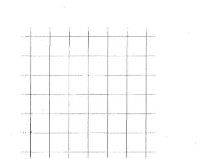
Definition 1.1. An n—grid array, is a framework of regularly spaced lines parallel to each of the coordinate axes, resulting in the division of Euclidean space into n-cubical sections.
Figure 1.1 shows a 6 x 6 zoom of a grid array in the plane. We use the arrays to represent the pixels (in two-dimensions) and voxels (in three-dimensions) that make up the images studied. In this work we shall consider binary arrays of values either 0 or 1. For purposes
Figure 1.1: A 6x6 segment of a standard grid array in 2-dimensions
of clarity, we adopt the convention that the value zero represents a white pixel while one will represent a black pixel. While it is possible to study gray-scale images using fuzzy
digital topology[KR89], any gray-scale image can be thresholded to give a binary image,
as such we limit ourselves to consider only binary images.
Each square of the grid array is assigned to represent a single pixel of a given image. Note that unlike a complex representation no care is taken here to represent the edges and vertices which make up a pixel, only the open squares are considered here. Since the grid array is of infinite size, (unbounded in all directions), we take on the convention that all squares not shown take the value zero and hence, represent white points.
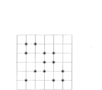
By convention when displaying images, instead of drawing in shaded an unshaded square, a time consuming task, a dual lattice representation of the grid array is created in which the lattice points represent the squares of the grid array and are colored accordingly. For clarity these lattices are joined by horizontal and vertical lines. These line perform no other function beyond esthetics. From now on we shall study images using their lattice representation, see Figure 1.2.
-© --© --© --© © © --© • -: * * ' : - •- • — • - • -© --© -•- •' --© -- • •- • - • -© --© --© - 1 1 © -• © © • © --© --© --© --© --© © --© --© ©
-Figure 1.2: A 6x6 pixel binary image where the black pixels are represented by the shaded
regions. The dotted grid is the array, note that the solid circles on the lattice points correspond to the black pixels of the image.
In order to study the lattice structures we must first implement the concept of a neigh-borhood.
Definition 1.2. An n-neighborhood of a lattice point, x, to be the n+1 lattice points geometrically closest to x under the Euclidean norm1, ||-||2.
There are many types of neighborhoods which can be defined. On the plane there are two neighborhoods that are commonly used, namely the A-neighborhood and the
8-neighborhood. These neighborhoods are defined by associating each lattice point a
co-ordinate in the two dimensional discrete plane N2. The standard convention is to write
Nm(p) when referring to the set consisting of the lattice point p and its m-neighbors.
Using this fact the ^.-neighborhood (Figure 1.3) of a lattice point x = (#i,X2) is the set of lattice points;
N4(x) - {(yi,y2)| \\(yi,y2) - (xux2)\\ < 1}.
1 Although here the Euclidean norm is used it is just as simple to use other norms more common to
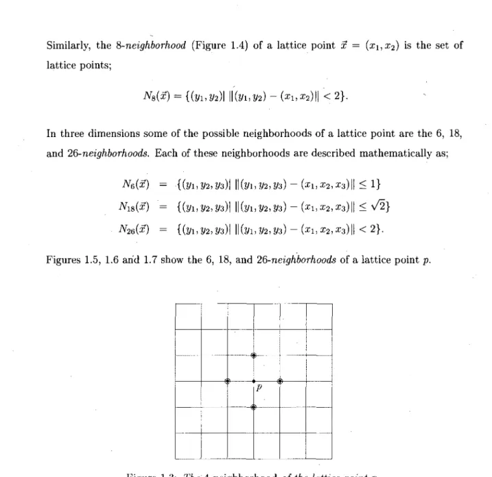
Similarly, the ^-neighborhood (Figure 1.4) of a lattice point x = (xi,x2) is the set of
lattice points;
Ns(x-) = {(yuy2)\ || (2/1^2) - (xi,x2)|| < 2}.
In three dimensions some of the possible neighborhoods of a lattice point are the 6, 18, and 26-neighborhoods. Each of these neighborhoods are described mathematically as;
Ne(x) = {(2/1,2/2,2/3)! IK2/1,2/2,2/3) - {xi,x2,x3)\\ < 1}
Ni8(x) = {(yi, 2/2,2/3)1 11(2/1,2/2,2/3) - (a;i,x2,a;3)|| < V2}
N26(x) = {(2/1,2/2,2/3)1 IK2/1,2/2,2/3) - (zi,x2,x3)\\ < 2}.
Figures 1.5, 1.6 arid 1.7 show the 6, 18, and 26-neighborhoods of a lattice point p.
V
Figure 1.3: The 4-neighborhood of the lattice point p.
Using the concept of neighborhoods we can define a relation between lattice points.
Definition 1.3. Two lattice points, x and y, are said to be n-adjacent to each other if and only if x is part of the n-neighborhood of y or y is part of the n-neighborhood of x.
.#>.-$ _*_
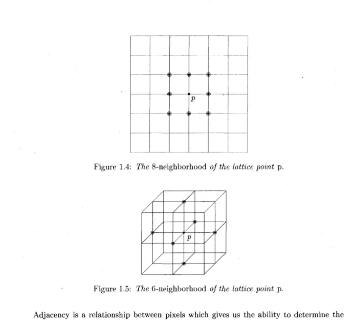
Figure 1.4: The 8-neighborhood of the lattice point p.
/
Zi-7
Figure 1.5: The 6-neighborhood of the lattice point p.
Adjacency is a relationship between pixels which gives us the ability to determine the structure of images. Knowing the concept of neighborhoods, and adjacency allows us to define a digital topology version of the topological concept of connectedness. From the concept of connectedness we will attempt to build a theory of "digital topology".
Definition 1.4. We define a sequence, P, of lattice points on an array, starting at a point p and ending at a separate point q, as an n-path iff each lattice point is n- adjacent to exactly two other lattice points in P with the exception of p, and q who are each n- adjacent to only one other lattice point in P. The case where p = q is defined as the
. / / /
y
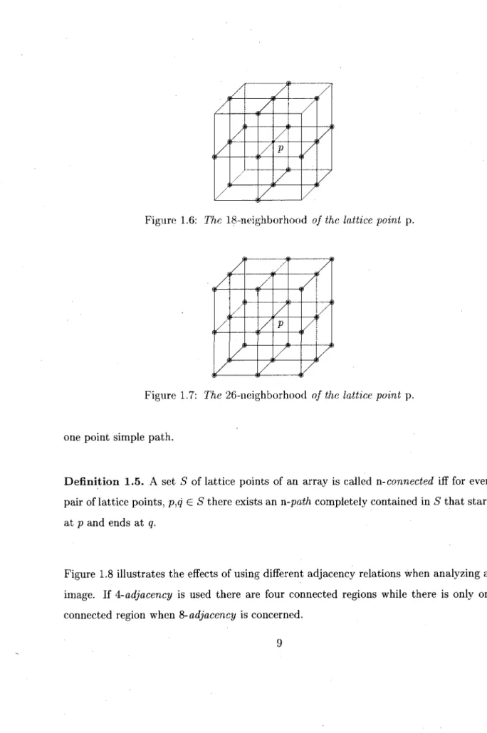
/ S— 1 i / ' V / / / /Figure 1.6: The 18-neighborhood of the lattice point p.
, / I / J / / p > / /- , / / / '
}
Figure 1.7: The 26-neighborhood of the lattice point p.
one point simple path.
Definition 1.5. A set 5 of lattice points of an array is called n-connected iff for every pair of lattice points, p,q G S there exists an n-path completely contained in S that starts at p and ends at q.
Figure 1.8 illustrates the effects of using different adjacency relations when analyzing an image. If ^adjacency is used there are four connected regions while there is only one connected region when 8-adjacency is concerned.
Hfc
$-•••&•
- 4
<*>--<$>
6
-4 fr
•4>~• $ - - $ <$>~
Figure 1.8: An 8-connected set with four ^components.
1.2 Digital Pictures
The most important concept in digital topology and the starting point for all research in the field are digital pictures (Definition 1.8). Digital pictures take the notions of digital topology, seen above, and combine them in a way that allows us to analyze digital images using classical topology. The first thing to keep in mind when wanting to analyze digital images is that they exist in a discrete space. Thus it is important that we construct digital images such that we are able to translate most of the concepts known in Euclidean spaces. The most fundamental concept in topology that one needs to translate to digital topology is the well-known Jordan Curve Theorem.
T h e o r e m 1.6. Any simple closed curve separates the plane into two domains, each having the curve as its boundary. One of these domains, called the interior, is bounded; the other, called the exterior, is unbounded [SS03]. •
The simplest example of a closed curve in a discrete space such as that of digital pictures would consist of four 8-adjacent points that are not 4-adjacent (Figure 1.9). If we were to
consider both the foreground and background with 4-connectivity, the black points would be totally disconnected but the plane would be separated into two domains. Alternatively, if we consider both the foreground and background using 8-connectedness the black points would be considered a simple closed curve, however the plane would not be separated into two separate domains. It would seem that we have no ideal way of analyzing this most simple of digital curves without running into some immediate problems. Hence, digital pictures were introduced to solve this fundamental problem by means of restructuring the way we look at a digital image.
— © ©—-—© o © — 0-<P 0-<P 4> 0 $ © ffi © ffi © $ $ (B © ©• © © © - 6 ©• 4 4>- -$-A .
Figure 1.9: The Jordan Curve Paradox for discrete spaces.
Definition 1.7. A digital picture space (DPS) is a triple (V,P,u), where V — 1? or
V = Z3 determines the dimension of the array, and (3 (UJ) is the set determining the
neighborhood relation of the black (white) foreground points usually [GDR04].
Definition 1.8. A digital picture is a quadruple / = (V,/3,u>,B) where (V,/3,UJ) is a
DPS and B is a finite set of black (or foreground) lattice points [GDR04].
The main feature of digital pictures is the association of "compatible" different adjacency relations to the foreground and background components of the image. This automatically
solves the Jordan Curve problem but brings about different ways of analyzing an image. Consider the image presented back in figure. 1.8. If we were to embed it in a (4,8) DPS we would see it as having four different foreground regions and one background region. However, if we were to use an (8,4) connectivity pair we would see one foreground regions and two isolated background regions. Therefore, it becomes important to describe the specifics of digital pictures. First of all a digital picture V = (V,(3,UJ, B), is considered
two-dimensional or three-dimensional depending on whether V — Z2 or V = Z3. The
adjacency of points in a digital picture depends on the choice of adjacency relations used, typically (/?, u) = (4,8) or (8,4) if V = Z2 and (/?, u) = (6, 26), (26,6), (6,18) or (18,6) if
V = Z3. Two black points are adjacent if they are /? adjacent, likewise two white points
are considered adjacent if they are u> adjacent, when considering a (f3,u>) digital picture. When determining the adjacency between black and white points, the two are said to be adjacent if they are u> adjacent. Figures. 1.10 & 1.11 illustrate the adjacencies of the two most typical two-dimensional digital pictures.
© e e e o
Figure 1.11: The adjacencies in a typical (4,8) digital picture. Note that the black point
set is the same as in Fig. 1.10.
1.3 On Simple Closed Paths, Holes, Borders, and
Cav-ities
As simple closed paths are important when analyzing digital pictures we take the time to summarize a few of their important properties. These properties will be useful when discussing border following algorithms later on. We begin by defining a few terms that will be used throughout this section.
Definition 1.9. Let A = (x0, • • • ,xn) be a set of black points satisfying the following
conditions;
1. n > 4;
2. xr = xs if and only if r = s;
3. xr € Ni(xs) if and only if r = s ± 1 or {r, s} — {0, n}.
Such an A will be known as a simple closed i-path.
condition 3 tells us that A never brushes past itself, and that A is indeed a closed 4-path where xo is a 4-neighbor of xn. Condition 1 is there to eliminate the pathological cases
where A is a singleton, 2 neighboring points or the 2 x 2 square.
Definition 1.10. Let x = (a,b) be any element of the complement of A, denoted A. Define the horizontal right half-line emanating from x as:
«x = {(a + A:, 6)|fc = 0 , 1 , 2 , . . . } .
Thus, Hx n A will be the elements of A along the right half line Hx whose terms are
a + ki + 1,... ,a + hi + ri;a + k2 + I,... ,a + k2 + r2\- •• such that 0 < k\ + 1 <
k\ + 7*1 < k2 + 1 < k2 + r2 .... This notation is used such that each ki is the starting
point of a run of elements in A on Hx of length rt. In figure 1.12 we have selected
a point x = (a, b) to the left of a closed curve. The right half line emanating from
x intersects the closed curve 4 times and as such the set A D Hx contains elements
{(a + h + 1, b), (a + k2 + 1,6), (a + k3 + 1, b), (a + k3 + 2,6), (a + fc3 + 3,6), (a + k4 + 1, &)}.
As such ki = 0, k2 — 2, fc3 = 4, k4 — 9; also, since there is only one "run" of length
greater then 1, r\ = r2 = r4 — 1 and r3 = 3.
If we investigate the behavior around a set of points {xu+x = (a + k + 1, 6),..., Xk+r —
(a + k + r, b)} (subscripts are modulo n + 1) of a run along Hx knowing that consecutive
elements are 4-neighbors allows us to say that the points Xk and xk+r cannot be located
on the bth row. Knowing this we can conclude that xk = (a + k + 1, b ± 1) and Xk+r =
(a+k + r, 6±1). We say that Hx touches A along the run {x^+i = (a+fc + 1,6), ...,Xk+r =
(a + k + r, b)} if both ±'s are positive, or negative, and that Hx crosses A along the run if
one is positive and the other negative. Keeping track of the number of times in which Hx
crosses A we can say that x is in the inside of A if we have an odd number or that x is
in the outside of A if we have an even number. Now that the notation has been clarified we quote the following propositions, which were initially described by A. Rosenfeld in
x
Wk • H W
n: •d
Figure 1.12: A possible simple closed 4-path in gray and purple with right horizontal
half-line Hx outlined in red. The elements of AC\HX are drawn in purple.
[Ros70].
Proposition 1.11. The inside and outside of any simple closed 4-path are both nonempty.
Proof. Gall A a set of black points satisfying definition 1.9. Because A is a subset of a
digital picture space, P of infinite size (in both the vertical and horizontal directions) we can always find an element x € P \ A which is further right than any element in A. Since x is to the right of any element in A, the right half line emanating from x will never contain an element of A, so by definition 1.9 x is outside A, hence the outside of
A is non-empty. To show that the inside of A is never empty take the set of uppermost
elements of A from them take the farthest right element. That is, Xh = (u, v) € A such that the corresponding elements (u + l,v),(u,v + l) are in P\A. The elements (u — l,v) and (u,v — 1), must be in A, since they are the only possibilities of xh-i, and Xh+i- By
condition 3, we know that (u — 1, v — 1) cannot belong to A, if it did it would mean that
Xh is allowed to neighbor more then two elements in A. Since A must be a closed path,
We conclude that (u — l,v — l) must belong to the inside of A and as such, the inside of
A is nonempty. •
Definition 1.12. Given two sets X and Y in a digital picture V — (V, ft, to, B) where X is a connected set, we say that X surrounds Y if each point of Y is contained in a finite component of V\X [KR89].
The concept of surrounds has several important properties in a digital picture V =
(V,(3,u>, B). It is easy to demonstrate that X surrounds Y is an antisymmetric (that is, aRb =S> bj$a if a ^ b for a given relation R), non-reflexive, transitive relation and thus, is
a partial order on the connected subsets of K[KR89].
T h e o r e m 1.13. In a connected digital picture, if a connected set of points X surrounds a connected set of points Y, then Y does not surround X.
Proof. Y is finite and connected, and since we work in a digital space, Y has a finite
number of finite components and one infinite connected component. To visualize intu-itively, one can draw a simple closed path,P, such that Y and the finite components of Y are located inside P , while the infinite component of Y is outside P. If we assume that
Y surrounds X, then X must be contained in a finite component of Y, call it A. Thus, X is inside P. Since X is inside P, and Y must be contained in a finite component of X, call it B, B must be adjacent to the infinite component of X. If B is adjacent to the
infinite component of X it is an infinite component, this contradicts the property that
X surrounds Y. •
Definition 1.14. In a digital picture V , a white component that is adjacent and sur-rounded by a black component C is called a hole in C if V is two dimensional and a
Q Q- ...©_ -Q <?~ -<P
• 4 $ - -A
<b- -$
0$• 0
-6 e- e- •<±> 6 - ~4>
Figure 1.13: A black component with two holes in an (8,4) "picture and one hole in a (4, 8) picture
Definition 1.15. In a digital picture V = (V,(3,u>,B) a black point p is said to be
isolated if there exist no black points in B that are adjacent to p [KR89].
Definition 1.16. Given a digital picture V — (V,P,u,B) with a connected black com-ponent C C B, any point p 6 C that is adjacent to a white point is called a border point (recall that in this case adjacent means w-adjacent). The collection of points p G C that are adjacent to white points is called the border of C in V . Given a white component
D € (V \B) the border of C with respect to D is the collection of all points in C that
are adjacent to D [KR89].
As a side note any black point which is neither a border point nor an isolated point is called an interior point. Figure 1.15 illustrates the three different types of black points.
... --W- -W-- -V _0_ _0_ -0- -0 $ - 0" 0
0-'0-:
0" ...4) ~0 $ ~0 0 0 0 0 0 0 0 0 0 0 6 e e e 0 0 0Figure 1.14: In a (4,8) digital picture, both p and q are isolated points while only p would
be isolated in an (8.4) picture
Simple Points, Thinning and Shrinking
Often some tasks in image processing are simplified when using fewer points. However, we must be careful to make sure that while reducing the image one does not make the mistake of changing it on a topological level. Thus, we must formulate rules that will allow us to remove or "delete" black points without changing what is important about the image on a topological level. In order to clarify the notation it is a good idea to define the following concepts.
Definition 1.17. Given a black point p from a digital picture V = (V,/3,UJ,B), we say that the point p is deleted from V when p is removed from the set B. In other words p is changed from a black point to a white point when it is deleted. In contrast, a white point q is said to be added to V if q is added to the set B.
f « <m 4 4 4 & 8} ® <$>• #• 4 4 <fe <k $ <fc <k (fe - * * — a ) BP m <® 4 <?> m + m # • • -# ® <*> m 4 * --§> -# 5) 4 <*> # 4 4 - • -*-- < • <$i- 4 Figure 1 encased only.
.15: Borders points of the (8,4) digital picture are indicated by the black points
in squares and circles, whereas the (4,8) border points are incased in squares
Definition 1.18. Given V = (V,/3,LO,B) and Vl = {V,0,u,B - D) two related digital
pictures, such that D C B. Then Vl is obtained from V by deleting the points in D. Conversely, V is obtained from Vl by adding the points in D [KR89].
There may be some confusion when talking about keeping an image unchanged in the topological sense when deleting or adding points, the following criterion clarifies this concept.
Criterion 1.19. Given V = (V,@,UJ,B) a two dimensional digital picture. Then the
deletion of any point p in the subset D of B preserves topology if and only if:
1. each black component of V contains exactly one black component of Vl,
2. each white component of Vl contains exactly one white component of V,
It is important to note that the above criterion ensures that the image remains unchanged at the topological level. However, it is not enough to ensure that the reduced image will hold all the important information found in the original. Although we are making sure that no holes are created or eliminated, criterion 1.19 is not complete. For example given a digital picture consisting of a simple black arc, as in Fig. 1.16, and proceeding to eliminate all black pixels such that criterion. 1.19 is satisfied we could possibly reduce the arc to a single point.
- o — < & •
(a) Before Shrinking (b) After Shrinking
Figure 1.16: A simple black arc in an (8,4) DPS can be reduced to the single point p
while maintaining the conditions of Criterion 1.19.
Any feature that is not preserved according to criterion 1.19 is said to be a non-topological requirement. Any algorithm which only considers the requirements of criterion 1.19 is known as a shrinking algorithm since if carried to the end the algorithm would shrink an image down to the smallest number of black points which would maintain the topological structure, (this was proved by Rosenfeld in [Ros70]). When the main goal is to keep non-topological requirements such as arc length, is accomplished by what are known as
thinning algorithms.
level. The requirement for a simple point is that it satisfies criterion 1.19 such that when a simple point p is deleted, the number of black and white components remains unchanged. Rosenfeld [[Ros70], section 3] presented a characterization of simple points which we now state.
Theorem 1.20. Let p be a non-isolated border point in an (8,4) or (4,8) digital picture. Let B be the set of black points of the digital picture and let B' = B — {p}. Then the following are equivalent:
1. p is a simple point.
2. p is adjacent to just one component of N(p) fl B'.
3. p is adjacent to just one component of N(p) — B.
Where N(p) represents the neighborhood of the point p.
As it may be unclear from the theorem, when we refer to the point p as adjacent to a component in an (m, n) picture, we mean m-adjacent to a black component and n-adjacent to a white component as outlined in the definition of adjacency. This theorem implicitly shows that only the immediate 3 x 3 neighborhood, N(p), of a point is required to determine whether a point p is simple or not. Another curiosity of this theorem is that a point p is a simple point of a digital picture (Z2,(3,OJ,B) if and only if it is a
simple point of the complement digital picture (Z2, j3, u>, (Z2 — B) U {p}). The latter can
be realized by swapping the black and white point sets of the former digital picture while keeping p a black point, as demonstrated in Fig. 1.17.
Edge Tracking Algorithms
Identifying the border of a digital picture is important in object detection and image thinning. The concept of a border here does not directly correspond to the border in
Figure 1.17: On the left the digital picture (Z2,8,4, B) with p as a simple point. While
on the right we have the complement digital picture (Z2,8,4, (Z2 — B) U {p}) where p is
still a simple point.
Euclidean space. We recall the classical definition of the boundary of a subset of a topological space.
Definition 1.21. The boundary of a subset A of the topological space T is the set,
cl(A) n (T — A), where cl(A) is the closure of A, and A is the complement. If T has a
metric the boundary of A is the set of all points at zero distance from both A and A [Lef49].
Since we have not defined any of the concepts such as closure, complement and metric in digital pictures, this definition lacks the description required here. If we were to try and force the use of this definition by embedding our digital picture into a Euclidean space we would not obtain our desired result either. The problem is that the topological boundary of a set S is of dimension one less then the set itself. Thus for a digital picture we would classically consider its edge as its boundary which is a problem since a digital picture is simply a collection of pixels all of which are of the same dimension. Figure 1.18 demonstrates the difference between an edge and the boundary which we want for a digital picture.
<k <k \s I a a> $ $
<$>
<$ $ m
<$ <$> $ ^~•4 -3H a ) ® ® ® ® ® ® ® ® $ <$> <$> ® $> $ $ <3> <¥> - *
Figure 1.18: Under (4,8) adjacency the boundary of the black point set S are the circled
and squared points, if we consider a (8,4) adjacency only the circled points make up the boundary. The edge of S is the green curve surrounding the set, which cannot be encoded by the lattice points.
In [Ros70] Rosenfeld declared a way of representing an edge using the pair of 4-adjacent pixels which shared it, obviously one of the pixels must belong to S while the other must belong to S. Thus, this notation allows for the use of an edge following algorithm. It is now possible to find the edge of a connected set S by using the "left hand on wall"technique, and S will be outlined in a counterclockwise manner. If the. set S is 4-connected then the algorithm begins with an edge e^ = (xk,yk), and without loss of generality we can say that Xk = 1 is to the left of yk = 0 thus we have the configuration , where a and b are the two pixels directly above. The process of "keeping one's left hand on wall" is accomplished by the proper choice of the the edge ek+i =
a 0 1. 1 b 0 1 %k+i xk a b Vk+i a b Vk
Columns a and b outline the possible values that the pixels directly above the edge can have, while the next two columns tell us which of the four pixels in the configuration
Xk = 1 and yk = 0 should be. Rosenfeld also proved in [Ros70] that by reiterating this
table until we arrive -back at the original edge efc gives us the complete set of edges to the set S. It is also possible to use the "left hand of wall" technique for an 8-connected set S if we use substitute with the following analogous table.
a 0 1 b 0 0 1 Xk+l Xk a b Vk+i a b Vk
Border Tracking Algorithms
It is also possible to create an algorithm that tracks the border of a connected set S instead of its edge. This has the advantage of taking fewer steps; for example when tracking the edges of an endpoint the 3 edges of the pixel must be visited, while in border tracking the end point is visited only once. On the other hand, as we shall see, border tracking algorithms are more complicated. Border tracking algorithms, like edge tracking, begin with the assumption that one border pixel has already been found. The algorithm itself then finds another border point by examining the neighborhood around the original pixel. The following section will describe a possible border tracking algorithm developed by Rosenfeld in [Ros70].
We begin with the initially known border pixel x0. To find the next border pixel x-y we
examine N^xo), for an element, 2/1 G Ni(xo) D S. Since x0 is a border point evidently
N4(XQ) n S will be non-empty. Number the pixels in N&(XQ) as j / i , . . . ,yg in a
counter-clockwise fashion, (figure 1.19). If none of 2/3,2/5,2/7 G {jto+i} belong to S then £0 is the
only border point.
— © © -© © e © $- 0-d>~ * -2/2 2/3 2/4 2/i X Q - $ 7 0 0 2/8 2/7 2/6 © © © © © © 6
Figure 1.19: An example of the labeling of pixels surrounding the known border point a;0
of a i-connected set S.
Now we can choose xi to be either one of two cases. If y2i G S then Xi = j/2i+i; or if
2/2i G S then £1 = y^i- Both cases ensure that x\ will have a white point in N^xi). It is important to note that there may be multiple choices for x\ depending on our choice of 2/i. Referring back to figure 1.19 if the algorithm started with 2/5, then x\ would have been chosen as 2/6 • Rosenfeld points out that using this algorithm will visit in the same order each element of S that the edge following algorithm from the previous section would. Using the similarity the following theorem becomes self evident.
T h e o r e m 1.22. Let XQ be any 4-border element of the finite, simply connected set S, and let the sequence Xi,x2 )... be defined from the above border following algorithm.
Then there exists a smallest positive integer m such that xm = XQ and x + m + 1; and
every border element of S occurs either once or twice in the set {xo, • •• , xm — 1} with
the latter holding if and only if the element has just two nonconsecutive 4-neighbors in
S.
Another type of border following algorithm discussed in [Ros70], uses a "helical scan" to find border elements. This is a simpler algorithm to the previous but has other drawbacks as we shall see. The algorithm proceeds as follows. Given any border element x0 and the
choice of whether to proceed vertically or horizontally to the next element X\, the choice of xi+i goes as follows:
1. if Xi e S turn right;
2. if Xi 6 S turn left;
3. If this is the third time in a row that the same direction has been taken, take the other.
Border elements can be read of the sequence of elements {x0, X\,..., xm} from the
algo-rithm. A border element Xi € S can be identified from the sequence if one of either xt-i
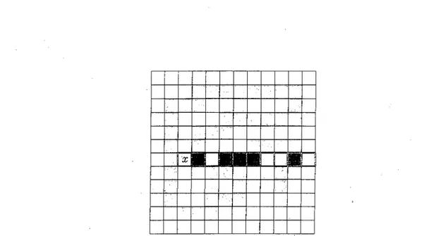
or xi+i in an element of S. Figure 1.20 illustrates the implementation of this algorithm
on a simple set.
The outcome of this procedure gives us a sequence of points, (XQ, 2/1, 2/2, 2/3, %o, £5, 2/6, 2/7,
x&, 2/9,2/10, £11, 2/12, 2/13, ^14, Z15, 2/16, 2/i7, 2/i8, ^15 after which it repeats itself). We use the
notation that an x represents a black point and a y represents a white point. Although trivial in this case, the border point can be extracted from the sequence anytime that an
x is adjacent to a y, and obviously here we end up with the border points (x0, x5, xs,
Xn, xu, and x15). This is not the most efficient algorithm for finding border points, and
....©... © ?> - < ? © © © © ©••• $• < * > • O $-h/i 2/14 ! / i i 2/17 -© $ <P - f <f> 0 2/13 - © Q>-1 3/Q>-12 © - © © © $ © (j) ?/io -© © © © e ©
Figure 1.20: An example of the implementation of the "helical" algorithm starting at the
point XQ and initially moving vertically upward.
There is also a problem in having the algorithm consistently identifying either a 4 or 8-connected component. In the simple case of a point set S made of 5 points that are 8 connected but not 4 connected, the algorithm does not stay on any single point as it should in a (4,8) picture, neither does it visit all points as it should in an (8,4) picture. Figure 1.22 illustrates this example but, instead of labeling the points arrows are used to follow the progress of the algorithm. Keep in mind that the algorithm ends when it reaches the initial point such that the next turn is a duplicate of the initial direction. Not only does the algorithm not visit every border point if initialized at the center point, but if any other initial border point is chosen the algorithm, will fail to identify all points of the connected component, no matter the initial direction chosen. Figure 1.23 shows the behavior of the algorithm if one of the corner border points is chosen as the starting point instead.
9
9-$ < 9-$ > • <t> & $ $. $ fc 6 <*>-2/5 ye 2/9 cp e <&• o -•j/io -e-•9 <5>-2/23 - $ r yn 2/22 J/14 <±> <*> 0 $ ^ 2 0 *fc 0-
J/19 0;- 0 'J/16 e « J/15 6 <*)Figure 1.21: The helical method on the same set as above but with a poor choice of initial
direction.
1.4 Euler Characteristics a n d Continuous Analogs
The Euler Characteristic of a polyhedral set,S, is a topological invariant in mathematics, and as such it would be nice to apply it to the construct of digital pictures. We begin by defining the Euler characteristic of a polyhedral set using a set of consistent axioms. By a polyhedral set we mean a set consisting of a finite union of points, closed straight lines, closed triangles, and closed tetrahedra.
Q © - - © © © © © © © © © © -<K- - A ~© -4) ©-- -dw--***- •--© © © ©-- • • • • * « - -*0-© &~ ••* :r0 -*•*--$*• »© © -- 4 * . -•*- - © © --© ©~ -*S> 0 -&- - * - ©--- e — ©• e © - - e © © ©~
Figure 1.22: On the left side the algorithm starts at x0 and initially moves vertically
the result is that the top right and bottom left points are not visited. On the right the algorithm again starts with x0 and initially moves horizontally and as a result the top left
and bottom right are not visited.
Definition 1.23. The Euler characteristic denoted x{S), of a polyhedral set S is an integer satisfying the following axioms,
1. X(0) = 0;
2. x(S) — 1 if S is non-empty and convex;
3. for all polyhedral X and Y, x{X U Y) = x{X) + x(Y) - x(X n Y).
Explicitly, x(S) is equal to the following alternating sum for an arbitrary triangulation of S:
(* of points) — (* of edges) + (# of triangles) - (# of tetrahedra) [KR89].
In fact if S is a planar (2D) polyhedral set then x{S) is simply equal to the number of connected components of 5 minus the number of holes in S. Take for example a 3 holed donut, it has 1 connected component, and 3 holes. Therefore, the Euler characteristic would be 1 — 3 = —2. In 3D, x(S) is equal to the number of components of S plus
H j * -< * H -$*-fx0 • * $ • • • • -*&--
-$*-I—4*r^
.TO » * -- A « -- - • $ - - e s> -»$- A A $-Figure 1.23: On the left side the algorithm starts at x0 and initially moves horizontally
the result is that the top left and bottom right points are not visited. On the right the algorithm again starts with .x'0 and initially moves vertically and as a result only the
border point x0 is visited. Due to symmetry the choice of any other corner as a starting
point will result in similar results.
the number of cavities of S minus the number of "tunnels" of 5. Figure 1.24 illustrates a cube missing to opposing faces, which would have 1 connected component, 0 cavities, and 1 tunnel. Hence, x(5) = 1 + 0 - 1 = 0.
The concept of Euler characteristics is well known in the field of algebraic topology. In order to apply it to the digital topology we introduce the idea of a "continuous analog" to a digital picture.
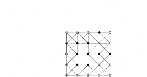
Definition 1.24. Let v be an (m, n) digital picture, where (m,n) — (4,8) or (8,4), we define the continuous analog of v , denoted C(v ), as follows. Let Co be the set of black points of v , let C\ be the union of all straight line segments whose endpoints are adjacent black points of v , and let C2 be the union of all unit squares and, if (m, n) = (8,4), all (1,1, \/2) triangles, whose sides are contained in C\. Then C{v ) = C0UC1 UC2 [KR89].
Figures 1.25 and 1.26 illustrate the continuous analogs of a digital picture in an (8,4) and a (4,8) framework. The continuous analog C{v ), has three important properties [KR89].
1. All lattice points in a connected set of C(v ) correspond to a black connected set of v .
Figure 1.24: A simple cube with two opposing faces missing, of Euler characteristic 0.
2. All lattice points in a connected set of the complement of C{v ) correspond to a white connected set of the complement of v .
3. A black component D of v should be adjacent to a white component E of v if and only if the boundaries of the components of C{v ) and its complement that contain
D and E meet.
From these properties it can be established that if v is a 2 dimensional digital picture then
X{v) = x{C{v))
— (#of components of C(v )) — (# of holes in C{v ))
= (* of black components of v ) — (# of holes in v ).
Aside from using the continuous analog, the Euler characteristic of a digital picture can be computed using methods more accommodating to computer algorithms. For two-dimensional (4,8) and (8,4) digital pictures, a formula was provided by Gray [Gra71] to compute the Euler characteristic of a continuous analog of a digital image using 2 by 2 blocks of lattice points:
© © © 0 0 0 © 0 0 © F • < • < • e © © s © © © • • • > • • 0 © • • • • • # © • © • © © © f • • © • © © • © © © • 0 ®, © © © 0 © 0 © ©
Figure 1.25: The continuous analog of a (4,8) digital picture.
4W = n(Q1)-n(Q3)-2n(QD)
4Z = n(Q1)-n{Q3) + 2n(QD).
The notation used applies to "unit cells" of the form a . Thus, n(Qi) denotes the
c d
number of unit cells with exactly i black points, while n(Qo) represents the number of units cells of the diagonal type, , or
A general way to derive a formula for computing Euler characteristics was outlined in [TKR92]. Beginning with any two or three-dimensional unit cell K, let K° be the set of vertices of K, Kl be the union of edges of K, and if K is three-dimensional, let K2 be
the union of the six faces of K. Then for all plane polyhedra, P we can define;
x{P\K) = x{.PnK)-x{PnK
l)l2-x{PnK°)H,
and in the three dimensional case we define;
© © © 0 0 0 © © © C i=; • (=. m e © 0 s © © T • • • * © © • • • A 0 © •=> • • • • ) 9 0 0 • 0 © 0 • © © 0 0 © © © © © ©
Figure 1.26: The continuous analog of an (8,4) digital picture. The black points are the
same as those in figure 1.25
From the Inclusion-Exclusion principle it is easy to show that, for any two, (three)-dimensional polyhedral set P, x{P) IS simply the sum of x(P; K) over all unit cells
CHAPTER 2
Axiomatic Digital Topology
In the previous chapter we discussed what is referred to as the graph based approach to digital topology. This highly intuitive approach led to many advancements in digital topology, (image subsets, boundaries, e t c . ) . Despite these advancements the approach has led to certain inconsistencies in the theory most notably with subset boundaries and the like. The idea of axiomatic digital topology was proposed by V. Kovalevsky [Kov88], in the late eighties. The approach suggests encoding images as complexes instead of as simple graphs. Although less intuitive, the complex approach, as we shall see, eliminates the paradoxes which arise using the graph approach.
2.1 Inconsistencies in the Classical Approach
In section 1.2 we discussed the problems with using the graph based approach and satis-fying the Jordan Curve Theorem. The problem was resolved using digital picture spaces where different adjacency relations where given to foreground and background pixels. This solution does not lead to valid topological structure of the digital space, as the
space structure must not depend on the definition of the variable subsets of the space [Kov92]. Furthermore, such a binary adjacency relation does not solve the problem in non-binary images.
There is another inconsistency which arises when considering the border of a subset of a digital image using the graph based approach. Since the only elements encoded into the graph are the pixels (the 3-D case poses a similar problem), a border must be defined using elements of the same dimension as the subset itself. As was seen in section 1.16 the border becomes a strip two pixels wide which, conflicts with the idea that the boundary should be a thin curve. Trying to shrink the border to only one pixel in width produces two different ideas of a border that of the inner and outer borders, Fig. 2.1. Another important property of the border to a set is that, the border of the set must equal the border of the set's complement, being forced to use borders as defined in the graph approach makes this property an impossibility.
H
(a) (b) (c) Figure 2.1: (a) A subset of a digital image, (b) Its inner border in green and outer
border in blue under (4,8) adjacency, (c) Its inner border in green and outer border in blue under (8,4) adjacency.
Figure 2.1 gives an inner and outer border both of which are only 1 pixel wide but it still has a non-zero area. There is an immediate problem since the inner and outer borders do not coincide. In addition, the (4,8) border has the disadvantage that it is not connected in either the inner or outer case (recall that we must consider 4 adjacency for objects here), whereas the (8,4) border is not simply connected (again this would be under 8 adjacency) in either case [Kov92j. These paradoxes lead to the conclusion that the current idea must be changed. In section 1.3 we saw the treatment of borders using "cracks", or 1 dimensional elements, and encoding each via the binary pair of pixels which where incident to each crack. The purpose in the next section will be to improve upon the idea of using elements of different dimension to analyze a digital image using finite topological spaces [Kov05].
2.2 The Axioms of Digital Topology
To begin defining axioms for a digital topology it is important to decide what basic properties are required as a structure for the topological space. From studying the graph based approach we have learned that analyzing the pixels alone leads to an inconsistent theory. A natural addition to the graph approach is to add elements other then pixels to the analysis. A complex is a mathematical structure which can be used to represent elements of differing geometric properties. This would allow the edges and corners of pixels to be analyzed. Before defining the complex structure we begin by building a proper topology on a digital image.
Definition 2.1 (Digital Space). A digital space is a set S together with a collection H(e) of subsets of S called neighborhoods of e, assigned to each element e g S . Such a space is denoted as (5, {N(e)}e<Es).
Definition 2.2. N(e) is the collection of elements called neighborhoods of e with the following properties:
1. V N Gtt(e), eeN.
2 . V e e S , S G N(e).
3. If Nj G N(e)Vj G J then;
4. UNi...Nk€ H(e) then;
fc
p|^GK(e).
Definition 2.3. A space (S, {N(e)}e6s) is called locally finite if and only if for all e € 5
there exists N G H(e) such that iV = card(iV) < oo.
Proposition 2.4. In a locally finite space, for all e G S there exists a unique smallest neighborhood SN(e) G H(e) that is such that SN(e) < TV for all N G N(e).
Proof. For all neighborhoods TVj of e G S that are finite we can define nj = Nj. Since {rij} C IN (the naturals) there exists n0 a minimum of {rij}. Let iV0 be a neighborhood
such that No = no. TO show that N0 is unique, we proceed by contradiction. Assume
that NQ and N({ are neighborhoods such that:
l.JV{,JV;6N(e);
By the properties of neighborhoods we know that NQ n NQ G H(e) and moreover that
(NQ fl Ng) < n0 which contradicts are assumption that no is minimal. Therefore we can
conclude that N0 exists and is unique.
•
Definition 2.5 (frontier). The border, also called the frontier, of a non-empty subset T of the space S, denoted FR(T, S), is the set of all elements e of S, such that the smallest neighborhood of e contains elements of both T and its complement S\T.
Definition 2.6 (incidence). If b G SN(a) or a G SN(6) we say that the elements a and b are incident to each other.
Definition 2.7 (incident path). Let T be a subset of the space S. A sequence (a\, a2, • • •, a^),
a* G T, i — 1, 2 , . . . , k; in which each two subsequent elements(ai_i, a,), are incident to each other, is called an incident path in T from Oi to afc.
Definition 2.8 (connectedness). Incident elements are directly connected. A subset T of the space S is connected if and only if for any two elements of T there exists an incident path containing these two elements, which completely lies in T.
Definition 2.9 (neighborhood relation). We define the binary neighborhood relation N on the space {S, K(e)eeS} as aNb ^ a e SN(6).
Definition 2.10 (opponents). A pair (a, b) of elements of the frontier FR(T,S) of a subset T C S are opponents of each other, if a belongs to SN(b), b belongs to SN(a), one of them belongs to T and the other to S — T.
Definition 2.11 (thin frontier). The frontier FR(T, 5) of a subset T of a space S is called thin if it contains no opponent pairs. Otherwise the frontier is called thick.
Example 2.12. Figure 2.2 is used to illustrate the difference between what will be referred to as thick and thin borders. On the left side of Fig. 2.2 we have an image
represented using the techniques found in Chapter 1, as such, the entire space S is simply the collection of all 2-faces or pixel faces while the set of gray 2-faces represent the image itself. Since the edges and vertices are not considered, the only way to define a border is to do so by stating the pair of pixels which properly encompass the set of gray points. As seen below the resulting border is a collection of opposing 2-face pairs which are represented as a line joining a black 2-face to its paired white 2-face. From def.2.11 we can see that Fig. 2.2a represents a thick frontier.
In contrast, Fig. 2.2b is the same basic image, but we have given each pixel neighborhoods that consist of more then just pixels. As such, the 2-faces are encoded along with their corresponding edges and vertices. Using such a structure the set of elements defining the image are the gray pixels, and the edges and vertices which are part of the boundary of any of said pixels. The resulting border simply becomes the black edges and vertices seen in Fig. 2.2b. By Def. 2.9 we see that there are no opponent pairs in the border of figure 2.2b, and it is a good example of a thin border.
si
Wh-O—U-J
1
(a) (b)
Definition 2.13. We call a locally finite space {S, tt(e)e6S}, an ALF space if it satisfies
the following 3 axioms.
1. Axiom Dl.
3 e £ S such that SN(e) > 1. In other words, {S, H(e)eeS} is not the discrete space.
2. Axiom D2.
The border FR(T, S) of any subset T c 5 i s thin.
3. Axiom D2>.
The border of FR(T, S) is the same as FR(T, S) i.e FR(FR(T, S), S)=FR(T, S).
2.3 Relationship to Classical Topology
We remind the reader of the classic axioms of topology. Given a topological space S there exists a collection of subsets of S, called open sets, satisfying the following axioms [Kov06]:
Axiom CI. The entire set S and the empty subset 0 are open. Axiom C2. The union of any number of open subsets is open.
Axiom C3. The intersection of a finite number of open subsets is open. Finally, a last axiom is sometimes imposed known as the separation axiom.
Axiom CA. The space has the separation property.
The separation property normally takes the form of one of the following three types.
Axiom TQ. For any distinct points x and y there is an open subset containing exactly one of the points.
Axiom T\. For any two distinct points x and y there is an open subset containing x but not y and another open subset, containing y but not x.
Axiom T2. For any two distinct points x and y there are two non-intersecting open
subsets one containing x the other y.
Due to the definition of neighborhoods, ALF spaces automatically satisfy the first three axioms of topology. We shall see later how to go about defining open sets in an ALF space. The separation axiom of topology is not immediately deduced from the construction of an ALF space. However we shall prove that an ALF space does satisfy the T0 separation
axiom.
Theorem 2.14. A locally finite space, {£, N(e)eeS} satisfies the thin frontier axiom if
and only if the neighborhood relation is antisymmetric that is, for all a,b £ S where
a ±b:
aNb^bXa. (2.1)
Proof. If the space satisfies the thin border property then by definition of border there
are no opponent pairs in the border of any subset, T, of S. Thus we can conclude that for each pair of elements a,b & S;
a e SN(6) =>• 6^SN(o).
As such the neighborhood relation is antisymmetric.
We shall prove the second part by contradiction. Assume the neighborhood relation is not antisymmetric and that there are no opponent pairs. Since the neighborhood relation is not antisymmetric, there must exist a pair of elements a,b G S such that a ^ b, aNb and bNa. In such a case, a is part of the frontier FR({a},5') since SN(a) contains an element in {a}, namely a itself, and an element not in {a}, b. By a similar argument, b is
also in the frontier FR({a}, S). Therefore, a and b are an opponent pair and the frontier
FR({a}, S) is not thin, which is a contradiction. •
In order to relate to classical topology it is convenient to define the concept of an open set in an ALF space.
Definition 2.15. A subset O C S is called open in S if it contains no elements of its frontier FR(0, S). A subset C C S is called closed in S if it contains all elements of FR(C,S).
Lemma 2.16. A subset T c S i s open in S according to Definition 2.15 iff it contains together with each element a € T also its smallest neighborhood SN(a) [Kov06].
Proof. If the subset T C S is open then it contains no elements of FR(T, S). Suppose
that a € T and there exists b e SN(a), such that b G S\T. Then by definition 2.5 a £ FR(T, S) which contradicts T open. Therefore in order that T be open, T must contain the smallest neighborhood of all its elements.
On the other hand suppose that T contains the smallest neighborhood of all its elements. Then for every a G T, SN(a) C T, and thus there can be no element b € S \T that is also in SN(a). Therefore no element of T can be in FR(T, S), thus T must be open. •
2.4 Properties of Axiomatic Locally Finite Spaces
This section outlines certain general properties of ALF spaces, which were defined above.
Definition 2.17. Consider the relation a ^ b and a € SN(fe) for a,b € S. This relation is called the border relation, denoted < and can be read as "6 borders a" or "a is bordered by 6" if a < 6.
Lemma 2.18. If S is an ALF space and the border relation < is transitive, then S contains elements, which are bordered by no other elements (maximum elements).
Proof. Now consider three elements a, b and c such that a < b and b < c. Since B is
assumed to be transitive, the conclusion a < c holds, and thus, c € SN(a) and SN(6) C SN(c) since c is any element of SN(6). Since a is bordered by b, o^SN(6), and we can conclude that SN(a) contains at least one more element then SN(6).
We now consider the following sequence of elements where each element bounds the one to the right of it:
... < a<b < c< d < e... , (2.2)
Without loss of generality, if we begin with the element b from the sequence we know from the definition of a locally finite space that the cardinality of SN(6) must be finite. We also know from above that in this sequence,
SN(6) >WHd.
We can continue moving towards the right in the sequence knowing that the cardinality of the smallest neighborhoods are strictly decreasing. Since S is a locally finite space we can be assured that the sequence must stop at a rightmost element whose smallest
neighborhood will contain a single element namely itself. •
We have proven the existence of maximal elements in ALF spaces. Another useful type of element to have when we will get to Chapter 3 are minimal element or those elements which border no other elements. However, unlike their maximal counterparts, the exis-tence of minimal elements is not guaranteed by the construction of locally finite digital