Analytical Properties of the Mean Field in Many Fermion Systems

(1)

Zeitsehrilt fiir PhysikA Z. Phys. A - Atomic Nuclei 333, 263-270 (1989)

Atomic Nuclei

9 Springer-Verlag 1989

Analytical Properties of the Mean Field

in Many Fermion Systems

J. Cugnon t, P. Gossiaux 1, and O. Harouna 2

1 Universit6 de Liege, Physique Nucltaire Th~orique, Institut de Physique au Sart Tilman, Liege, Belgium

2 Universit~ de Niamey, Service de Physique, Niamey, R~publique du Niger Received January 24, 1989; revised version April 12, 1989

The importance of the dispersion relation linking the real and the imaginary parts of the mean field in many fermion systems is pointed out. General models are built for the imaginary part. The properties of the real part close to the Fermi level are discussed in relation with these models. Its analytical behaviour is determined by the analytical behaviour of the imaginary part in the same domain, but the numerical values can be strongly influenced by the large energy behaviour of the same quantity. The sensitivity upon the behaviour in the intermediate domain is described semiquantitatively. The nuclear matter case is briefly discussed. The generality of our results is pointed out. PACS: 21.65

1. Introduction

The fact that the energy dependence of the mean field in a Fermi liquid could show some particular behaviour near the Fermi level has retained the attention for a long time [1-3]. Recently, the interest was re- vived by the observation underlined by several au- thors that the nuclear shell-model does indeed display a kind of plateau close to the Fermi level in contrast to a general decrease in the energy dependence [4-7]. For a long time, it has been recognized that the real part and the imaginary part of the nuclear mean field are linked through a dispersion relation [3, 8]. Re- cently, it was shown that our knowledge of the imaginary part at low energy is more or less sufficient to predict the gross properties of the real part near the Fermi level through the dispersion relation [6, 7, 9]. However, the precise relationship between the global properties of the two functions has not really been clarified. For instance, it is not known whether the size of the effective mass (roughly the derivative of the shell-model potential) depends upon the local behaviour of the imaginary part of the optical-model potential only, or whether it depends upon this quantity for remote values of the energy. We propose here to study this problem for the case of an infinite Fermi

liquid, for which the situation is simpler because of translational invariance. Our idea is to study model functions for the imaginary part, for which the dispersion integral can be done analytically. We will study models for which the dispersion integral converges as well as those for which subtracted relations have to be employed. Furthermore, we will consider very general forms of the imaginary part, some of them are quite unrealistic for nuclear matter. However, we think that our results may be of some help for other problems of physics, in which similar dispersion relations are employed.

2. Theoretical Background

The propagation of a particle of momentum k and energy E in a uniform Fermi system can be described by the Green function G(k, E) or by the mass operator

M(k, E), the two being related by [10]

[ h2k2 ]-1

G(k, E)= E 2m M(k, E) . (2.1)

The mass operator, which can be considered as the mean field experienced by the particle, contains a real and an imaginary parts [2]

(2)

264 J. Cugnon et al.: Analytical Properties of the Mean Field which are related by the dispersion relation

V ( k , E ) = - f(k)+ P- +~ __W(k'E') dE',

(2.3)

rc -oo E'--E

where

f(k)

is an undetermined function, and where P denotes the principal value integral. The integral represents the Hilbert transform of W considered as a function of E [11]. Relation (2.3) is totally general and derives from causality only. The function

W(k, E)

is positive definite. A related quantity is the (energy) effective mass rfi, defined as

rh = 1 + ~

V(k, E).

(2.4)

The quantities (2.2)-(2.4) have no direct physical meaning. F o r a fixed value of k, the physical counter- parts are obtained by replacing E by

e(k),

the physical single-particle energy, i.e. the value of E where the Green function (2.1) has a pole. Alternatively for a given value e of E, the physical quantities can be obtained by replacing k by

k(e),

the inverse of the function

e(k).

Let us denote them by

V(e), W(e)

and nq(e). Strictly speaking, the physical quantities

V(e)

and

W(e)

are linked by a dispersion relation similar to (2.3) if and only if

W(k, E)

are independent of k. In practice, the k-dependence is very smooth, except for special unrealistic models [12], and relation (2.3) can be used with physical quantities as a first approach in the case of nuclear matter. It is even currently used [6, 7, 9] in the case of finite nuclei. Furthermore, the

analytical

behaviour in e (which will be important for our discussion) is not modified by introducing physical quantities. Our results will be nevertheless exact for off-shell quantities

(k+k(e))

and for m a n y cases, where the energy (or an equivalent variable as it is the case for dispersion relations used in different contexts) is the only relevant variable [7, 13-15]. Therefore, in the following, we will disregard the k- variable and use E as the running variable. We will denote it as the energy, but it may correspond to other physical quantities. We will use the following notations:

V(E) = - - f + V> + V<,

(2.5)

where (for convenience, the zero of the energy scale is set on the value of the chemical potential)

P ~ W(E')

, ~ ,

(2.6)

and where V< denotes the integral form - oo to 0.

In many perturbation schemes for the function W, the lowest order contribution corresponds to V>, sometimes named the polarisation contribution. The next order contributes to V<, named the correlation contribution.

If E < 0 in (2.6), the principal part loses its meaning and the integral reduces to the so-called Stieltjes transform. F o r the mathematical aspects of these transforms, see [16].

3. Non-subtracted Dispersion Relations

3.1. Introduction

We want here to discuss the following question: how is the behaviour of the polarization contribution V> close to the Fermi energy influenced by the properties of

W(E)

close to E = 0 , close to E = oo and in the intermediate region? We assume that

W(E)~O

at E ~ 0% so that the dispersion relation (2.1) converges. This case may not be relevant to nuclear physics, although we do not know really the asymptotic behaviour of the imaginary part of the optical model potential. However, this m a y nevertheless be important for other physical situations (see our discussion below).

3.2. Properties of V>

We are first interested to took at the effect of the behaviour of W at small energy. F o r this, we may consider the following model (E > 0)

W(E) = W o (E/Eo)" e- Era,

(3.1)

for different values of n. As long as the behaviour close to E = 0 is considered, the nuclear matter case, which will retain our particular attention (see Sect. 5), corresponds to n = 2 . However, we want here to be very general and attempt to derive general conclusions for many fermion systems, some of which may qualitatively differ from nuclear matter, because of either a different dimensionality of the system or a different nature of the interaction. In the case of (3.1), V> can be calculated from (2.6). The Hilbert transform is given in Appendix A. Using (A.3), one has, close to E ~ O

+27+]-+ ...} (3.2)

for n = 0 , where _+ refers to E > or < 0 . Then n = 0 case may not be an academic one. In the antiproton- p r o t o n system, the imaginary part is large and contin-

(3)

J. Cugnon et al.: Analytical Properties of the Mean Field 265 \ \

i ~ 1 .f----~_ -

/.._/

v:O.3 v=0.5 -/.~

~=1.3

--

p.=t5

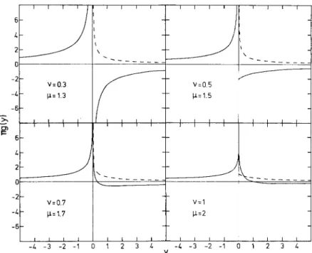
I I t I I I I J J I I I I V=I - - I X = 2 I I I I I I I y -A -6 V=O.7

p.=1.7 Fig. 1. Hilbert transform g(y) (full line), defined

as in (A.1), of the function x~-~(1 + x ) a - " (dotted line), for various values of the parameters v and #. See text for detail

uous through the threshold. As we show later on, this will reflect in a E In E term in the real part of the optical potential close to threshold. This might be related to the observed structure of the so-called p-parameter in the a n t i p r o t o n - p r o t o n scattering [-14].

One also has 1> - n Eo E2 4-... "(-+7-+'n ( + - ~ ) + ~ + " " ) ]

(3.3)

for n = 1, and v> =

W~

(n- 1)!+(n-2)!

(El) (E)n-1

... + \ ~ )

)]

for n > 2. The larger n, the smoother the function is a r o u n d E = 0.

As another model case, we chose

( E~ ~-1

(1

E\i-u

W(E): Wo \Eo]

+ ~ )

,

(3.5)

with E~ > 0 , # > v > 0 . Using (A.8) and the properties of the hypergeometrie functions, one can show that if v is not an integer, the following behaviour holds: if v < 1, V> will be divergent at E = 0 as y~- ~. If 1 < v < 2, V> will be finite and continuous at E = 0, with an infinite slope as y ~ 0 - , but not necessarily above.

3 i i V = l I 5 I I

F

J I I I I

Fig. 2. Same as Fig. 1

I I V=3 IX=/. j J I I (:~5) v=lO ~=11 ~ J Y I I I

If v > 2, V> is finite, continuous and linear at E = 0. F o r integer values of v, one can summarize the situation as follows. If v = 1, there is a logarithmic diver- gence at E = 0 . If v = 2 , the dominant terms are in y and y In y. F o r v > 3, the log term is in

y2

In y. These properties are illustrated by Figs. 1 and 2. As one can see from the comparison of the two cases (3.1) and (3.5) for v being an integer, the leading power

of

W(E)

will govern the analytic properties of V> close

to E = 0 .

N o w we inquire a b o u t the importance of the large E properties of

W(E).

F o r simplicity, we consider forms of

W(E)

which start a s E 2 or E. One possibility is provided by (3.1), for which one has expressions

(4)

266 J. C u g n o n et al.: Analytical Properties of the M e a n Field

(3.3) and (3.4) for the linear and the quadratic forms, respectively. Alternatively, we can consider

+E-7)

'

(3.6)

where ~ > 0. For n = 1, one obtains

t1>

WoE1

1 [ E ~- E0 ~ 1--r E~ § 1) (~-l) 2 (if(2+ 0 + ~ ; - - 1) E E 2 .], - { ~ - l l n ~ + { ( ~ + l ) ( ~ - l ) In ~--7+.. (3.7) where ~ is the Digamma function, while

Wo(Eq2 2 [

_{1+r EW}

( 0 ( 2 + 0 + ~ ) 2 2 ( ~ k ( 2 + 0 + 7 - 1) 2 2 (~ + 2) In + . . . (3.8)

stands for n = 2. It is evident, by comparing (3.7) and (3.8) with (3.3) and (3.4) respectively, that the fall-off of

W(E)

at infinity does influence the behaviour of V> at E,~0, although the

analytic

properties in that neighbourhood are still determined by the dominant power of E in

W(E)

close to E ~ 0.

An alternative way to investigate the importance of the fall-off at infinity is to look at the Hilbert transform of a function

W(E)

of the form

(Ez,

E~ > 0):

W(E)

= 0 for E < E2

= Wz

exp

[ -- (E -- E2)/E J

for E >

E z .

(3.9) F r o m (A.3) and the elementary properties of the Hil- bert transforms, one can write the Hilbert transform H(W, E) as

H(W,E)=WEexp[ E - E 2 ] E [ E z - E ~

rc E~ J 1\ E~ ] ' (3.10)

where E1 is the exponential integral. Close to E = 0 and for E 2 > E~, one can write

H(W, E ) - 14/2 E~ 1 - - E ~ E + . . . . (3.11) 7c E z

One can see that, in the limit

E2/E~--+

o% a perturbation in W will induce a small contribution to V> (E) close to E = 0 (even a smaller one to rfi), but one has to keep in mind that this contribution will no longer be negligible if E~,~ E2, even if E2 is very large.

The sensitivity of V> (E ~ 0) upon a modification of

W(E)

in the intermediate domain can best be stud- ied by considering the function

W ( E ) = 0 for E < E a , or

E2<E

( 0 < E I < E 2 )

= Wo c (p, 0.) ( E - E 1) p - 1 (E2 - E ) ~ - 1,

for E1 < E < E 2 (3.12)

where C(p, 0.) is a normalization constant

C(p,

o-) = [ ( E 2 -

El) p+a- 1B(p,

0.)] - 1, ( 3 . 1 3 ) which ensures

Ei

w ( E ) d e = Wo. Eo

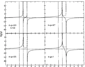
In expression (3.13), B denotes the Beta function. In- stead of analyzing the analytical properties of the Hil- bert transform (A.10), it is perhaps more convenient to look at the numerical illustration of Figs. 3 and 4, where various

p=0.

cases are shown. It is then clear that a discontinuity of the type ( x - a ) ~- 1 with 0 < 0.< 1/2 produces locally an infinite discontinuity with change of sign. If 1/2 < 0. < 1, the infinite discontinuity is logarithmic without change of sign. When

1

_< 0._< 2, the Hilbert transform is finite at y = a, with a form which becomes smoother and smoother as 0. increases, taking the y In y shape close to a and b as 0. reaches 2, in agreement with the similar case (3.7) that we discussed before. F o r 0->2, the Hilbert transform is finite at y = a and the derivative is linear. The Hilbert transform takes characteristic shapes for special values of 0.. The conclusion is that special analytical behaviours of

W(E)

have a direct and local consequence on the analytical properties of V> (E).

F r o m the above discussion and observation, we can make two statements:

(1)

the real nuclear mean field being likely a smooth function (except perhaps at E = 0 for components V> and V<), there should be no angular point in any representation of W(E);

(2)

the modification of

W(E)

at intermediate energy does influence the value and the behaviour of V> (E) around E = 0. It is however difficult to draw general quantitative conclusions. As an illustrative case, one m a y consider the circular (p = 0. = 3/2) and the para- bolic (p = 0. = 2) cases. Then the quantity V> (E) corresponding to (3.12) can be written (close to E = 0 ) as

(5)

J. Cugnon et al.: Analytical Properties of the Mean Field 267

6

-1 -2 -3 0 1 3 & 5 - 1 - 2 - 3 0 1 2 3 4 5 Y

Fig. 3. Hilbert transform g(y) (full line) of the function (dotted line)

C(p, o) ( x - 1 ) p- 1 ( 2 - x ) ~- 1, with C(p, ~) given by (3.13) for various values of the parameters v and /~. See text for detail. Note that g(y) = 0 for a = p =0.5 and 1 __<y__<2

1 i i -4 - 0 = p : 1 . 5 -E L i E g, E 4 [ -z - 0 = 0 = 2 -E J - ~ - ~ o Fig. 4. Same as Fig. 3

S F f f 0 = 9 = 3 I I I I I I I t j rl o = p = 1 0 l i l t Y and V~ ~ Wo ( E 2 - E1) 2 r E 1 / 1 E 2 + E 2 E ~ + E 2 [ l n E 2 2 - - E ~ (3.15) respectively. This is by no means negligible if E2

- E l > E l for instance.

3.3. Properties of V< and of V(E)

It has often been stated that the potential W(E) has a symmetrical shape in the nuclear case. As a matter of fact the behaviour close to E = 0 should be symmetric for phase space reasons [12, 171, except for very

pathological interactions. If W ( E ) = W ( - E ) , then V< (E) = -- V> ( - - E ) and therefore

v(E) = v> ( E ) - v> ( - E) (3.16)

which means that V(E) is an odd function of E. There- fore all the even powers of E in expressions for V> are preserved when going to V(E). F o r the terms con- taining a logarithm (which occurs regularly in the model cases above) of the type E" In E, only odd values of n will be retained. As a consequence, all possible logarithmic singularities in V> and V< are cancelling each other, leaving a much smoother E In E "singularity" in V(E).

4. Subtracted Dispersion Relations

If W(E) goes to zero as a constant (at the least) at infinity, one has to use subtracted dispersion relations of the type

A V> = V> ( E ) - V> (0) = E P ~ W(E')

o E ' ( E ' - E ) dE'. (4.1)

The results of Sect. 3 can readily be used to study the analytical behaviour of A V>. As a very simple example, let us assume that (0 < r < 1)

W(E) = Wo/~ (E/Eo) 2 (I + E / E , ) - ' + r (4.2) Then (3.6), (3.7) and (4.2) can be used to obtain

Wo El

AV> - E~

9 E - ( ~ + 0 ( 1 + 0 ) E I - E ~ . . . .

(4.3)

F o r a symmetrical function W(E) (from --oo to or), the quantity A V=A V> + A V<, will behave like (for E ~ 0 )

W o ~ e

A V~ 2 (4.4)

1~ E~ E 1 "

Another very commonly used example is provided by

E 2

W ( E ) = Wo E2 + E ~ ' (4.5)

for all values of E. The corresponding quantitiy A V reads

E 0 E

(6)

268

5. The Nuclear Matter Case

5.1. The Potential

The nuclear matter case would correspond to a func- tion W(E) which has to fulfill the following require- ments: ( 1 ) it is positive everywhere; ( 2 ) it behaves like E 2 close to E = 0. Nothing more can be said for sure at the present status of our knowledge. Very like- ly, W(E) does not go to zero at infinity, but the precise behaviour is not known. F o r the very crude hard sphere model of nuclear matter, it increases like E 1/2 when E--* oo. (The potentials which contain a strongly repulsive core seem to give [18] too large an imaginary part for intermediate energy, say between 40- 100 MeV.) On the other hand, there are arguments indicating that W(E) ~ a constant when E ~ - co. So, very likely, the function W(E) is not symmetrical. Therefore a plausible form is

W ( E ) = Wo(E/Eo) 2 (1 +E/Eo) -~ -r E > 0 (5.1)

= Wo(E/Eo) z (1 --E/E'~) -1-r E < 0 , (5.2)

with ~ and 4' lying between 0 and 1. Owing to (4.2) and (3.7), we obtain A V - W o E [[E 1 E'~\

0 , , + , , + , .

' 1 4 + 2

+ ( ~ - (~,( +4')+~- 1-1n IE'~I)

+ 4 + 1 ( 0 ( 2 + 4 ) + 7 - - 1 --In

lEvi))

E 2 / 4 + 1 4 ' + 1\ E2 ..

_(5.3)

The remarkable result here is the mutual cancellation of the E z in E terms contained in A V> and A V<. This results from the symmetrical behaviour of W(E) in E 2 close to E = 0 . In Fermi liquids, this behaviour, in turn, results from the phase space density of 2 particle-1 hole and 2 hole-1 particle states close to the Fermi level. This argument was already found by Migdal [19]. The E 3 in E singularity is thus typical of Fermi liquids and is to be compared with the T 3 In T singularity of the specific heat in liquid 3He [20] where, however, the imaginary potential arises from the coupling of the single-particle states with collective excitations, the paramagnons. Equa- tion (5.3) also displays the influence of the fall-off of

J. Cngnon et al.: Analytical Properties of the Mean Field W(E). In particular, it shows that a E 2 term arises

when W(E) is not completely symmetric at large

IEI.

5.2. The Effective Mass

By differentiating expression (5.3) and using (2.2), one can write the (energy) effective mass as

[E, El\ 2Wo (0 (1+ 4') -- 0 (1+ ~)

\

Once again, the influence of the large (positive and negative) energy behaviour of W(E) is evident in the leading term of th in the neighbourhood of E = 0. This can explain, and this is our most important conclusion, why different calculations although giving roughly the same imaginary potential at low energy can yield nevertheless different values for the effective mass [21-23].

Let us finally consider, for the sake of illustration, the case of the Paris potential, for which Wo/E~ 8.5 x 10- a MeV - 1. The calculated value of ff~(E = (3) is 1.7, according to [21]. If we assume expressions (5.1) and (5.2) we obtain from relation (5.3) E1/~

+ E'~/4 ~ 630 MeV, which looks as a reasonable value

for the " d e c a y constant" of the imaginary potential at large energy.

6. Importance of the Dimension

T h e E 2 behaviour of W(E) close to E = 0 arises from the three-dimensional character of the ordinary world. One may speculate on the possibility of other

j

Y

I I

-0.5 0 0.5

y

5. Hilbert transform g(y) of the function [ f x e -~ Fig.

(7)

J. C u g n o n et al.: Analytical Properties of the M e a n Field

dimensionality for fermion systems. In one dimension, the density of 2 p - I h states on the energy shell (real transitions) identically vanishes. F o r off-energy shell transitions,

W(E)

will behave like a constant. There- fore, the A V potential will contain a E In E singularity. F o r two dimensional systems

W(E)

behaves linearly. If this is true, the A V potential will contain a E 2 In E singularity.

Some of our considerations may be useful in other contexts. Just to give an example, dispersion relations of the types (2.3) or (4.1) come into play to describe the dispersive shifts of resonance states in reaction theory [24]. F o r s-wave states, the corresponding function

W(E)

starts like

E i/2

at threshold [25]. Ow- ing to (A.4)-(A.6), one sees that the corresponding function

V(E)

has a discontinuous derivative [26] at E = 0 (see (A.6)), as illustrated in Fig. 5.

7. C o n c l u s i o n

We have analyzed the dispersion relation connecting the real and imaginary parts of the mean field in a many-fermion system. We looked at several plausible models for the imaginary part and calculate accord- ingly the real part

V(E).

We illustrated the fact that the singularity of

V(E)

close to E = 0 is linked with the dominant power of

W(E)

close to E = 0. We stud- ied non-subtracted as well as subtracted dispersion relations. We tried to exhibit the effect of the large IE[ behaviour of the imaginary part and we showed that although it does not affect the

analytic

behaviour

of

V(E),

it can strongly modify the numerical value.

We particularly examined this point in relation with the effective mass and provide an explanation for the different values of the effective mass obtained by different calculations, although giving roughly the same mean field at the Fermi level. We also investigated semi-quantitatively the sensitivity of the real part of the mean field upon the value of the imaginary part in the intermediate energy domain. We made our considerations as general as possible in such a way that the conclusions can be applied outside the nuclear case which has attracted our attention.

A p p e n d i x : H i l b e r t T r a n s f o r m s

We here quote the Hilbert transform

H(W,y)=P ~ W(x) dx,

~ o x--y

(A.1)

269

of several functions

W(x)

which are of interest for our discussion. If

W(x)=x"e -ax,

(A.2)

one has 1 1)!

a-ry"-r],

H(W,Y)=;[--Y"e-"'EI(aY)+ ~=I(r--

y > 0 1 1- . ay = ~ - [ y e -

El(--ay)+ ~ (r-1)'a-'y"-r],

r = l y < 0, (A.3)

where E i and E~ are the exponential integral functions, with standard notation [27]. F o r v > 0 and

W(x)

= x ~ - i e - ax, (A.4)

H(W, y) = F ( 2 - v) y l -

VeaY

F(1 - - Y,

ay),

(A.5)

where

F(a, z)

is the incomplete G a m m a function. In particular, for v = 3/2, Y e" u]

H(W"y)=l--[(~--Ii/2rck\a]

- - ~ 2

e - " ' V Y ! 2 ~ d , y > 0 = 1

[ ~ a - ~ - - y e - " ' e r f c ( ~ - - a y ) ] ,

7~ y < 0. (A.6) F o r the function (a > 0, # > v > 0)

W (y) =- x v- i (x + a) 1 - u,

(A.7) one has H'W. " - r ( ~ - v) r(v)

t ,Y)- F~-~.=71

F ( / l - l , v ; / ~ ;

l+y/a)(-y) ~-~,

y < O

7rye- 1

F(li-- v--

1)

F(v)

- ( y + a ) U _ 1 c o t a n 0 z - - v ) n

(y + a) F(#- l )

-al-U+~F 2 - - / ~ , 1 ; 2 - - # + v ; , y > 0 , (A.8) where F is the Gauss hypergeometric function. We also consider (0 < a < b) the function

W ( x ) = 0 if x < a or

x>b,

(8)

270 J. Cugnon et al.: Analytical Properties of the Mean Field

with p a n d a > 0, for which one has

r(p) r(~) (b -- a) p + ~- 1

~/(W,y)=.r(p+a)

(b-y)

for

y < a

or

y>b,

= (y _ a)p- 1 (b - y y - 1 c o t a n (a ~)

r(p) r ( a -

1)

( b _ a ) p + ~ _ 2

~F(p + a -

1)

. F ( 2 - p - a ,

l ; 2 - a ; bb~Ya),

Finally, for the function

F (1, a, P + a; bb--~_ay),

a < y < b .

(A.10)

W(x) = x/(x z +

a2), (A. 11) one has (A.12)

10. Lifshitz, E., Pitaevskii, L.P.: Statistical physics, Part 2. Oxford, New York: Pergamon Press 1980

11. Courant, R., Hilbert, D.: Methods of mathematical physics. New York: Intersr 1953

12. Sartor, R., Mahaux, C.: Phys. Rev. C21, 1546 (1980)

13. Shirkov, D., et al.: Dispersion theories. Amsterdam: North-Hol- land 1969

14. Bugg, V.: Antiproton 86. Singapore: World Scientific 1987 15. Locher, M., Mizutani, T.: Phys. Rep. 46, 43 (1978)

16. Erd61yi, A., et al.: Tables of integral transforms. New York: Mac Graw-Hill 1954

17. Belyakov, V.: Sov. Phys. JETP 13, 850 (1961)

18. Lejeune, A., Grange, P., Martzolff, M., Cugnon, J.: Nucl. Phys. A453, 189 (1986)

19. Migdal, A.: Nucl. Phys. 30, 239 (1962)

20. Mota, A., Platzeek, R., Rapp, R., Wheatley, J.: Phys. Rev. 177, 266 (1969)

21. Grange, P., Cugnon, J., Lejeune, A.: Nucl. Phys. A473, 365 (1987) 22. Fantoni, S., Pandharipande, V.: Nucl. Phys. A427, 473 (1984) 23. Hasse, R., Schuck, P.: Nucl. Phys. A445, 205 (1985)

24. Jackson, D.: Nuclear reactions. London: Mc Thuen 1970 25. Lynn, J.: The theory of neutron resonance reactions. Oxford:

Clarendon 1968

26. Lane, A.: Phys. Lett. B50, 207 (1974)

27. Abramowitz, M., Stegun, I.: Handbook of mathematical functions. New York: Dover 1972

References

1. Brown, G.E., Gunn, J., Gould, P.: Nuel. Phys. 46, 598 (1963) 2. Jeukenne, J.-P., Lejeune, A., Mahaux, C.: Phys. Rep. 25C, 83

(1976)

3. Glyde, H., Hernadi, S.: Phys. Rev. B28, 3770 (1983) 4. Mahaux, C., Ng6, H.: Phys. Lett. 100B, 285 (1981) 5. Mahaux, C., Ng6, H.: Phys. Lett. 126B, 1 (1983)

6. Johnson, C., Horen, D.J., Mahaux, C.: Phys. Rev. C36, 2252 (1987)

7. Mahaux, C., Sartor, R.: Nucl. Phys. A468, 193 (1987)

8. Goldberger, M., Watson, K.: Collision theory. New York: John Wiley 1964

9. Lozano, M.: Phys. Rev. C36, 452 (1987)

J. Cugnon, P. Gossiaux Physique Nucl6aire Th6orique Institut de Physique

Universit6 de Liege Sart Tilman, B~timent B.5 B-4000 Li+ge 1 Belgium O. Harouna Service de Physique Universit6 de Niamey B.P. 10662 Niamey Republic of Niger