What is the actual conductor temperature on Power Lines

What Is the Actual Conductor Temperature on

Power Lines

Salima Balghouzal

, Jean-Louis Lilien

, Mustapha El Adnani

1, 2_{University of Liège, Department of Electricity,Electronics and Computer Sciences, Sart Tilman B28, Liège, Belgium} 1, 3_{University of Cadi Ayyad, National School ofApplied Sciences, Av Abdelkarim El Khattabi, Gueliz, Marrakech, Morocco}

1_{Balghouzal.s@gmail.com;} 2_{lilien@montefiore.ulg.ac.be;} 3_{eladnani@uca.ma}

Abstract- Power lines are thermally designed for decades using standards and sometimes advanced simulation tools. They are using conductor temperature as a key factor for clearance determination. But what is conductor temperature when we all know about temperature changes along the line, even inside one span, circumferential temperature gradient and radial gradient inside the conductor, especially with new type of high temperature conductor, none of existing methods are able to give a fully clear picture of temperature action on the multi-span line along its everyday behaviour. Actually sensors are coming on the market of dynamic line rating, using temperature sensors. These sensors themselves are introducing significant local effects. What is actual link between ampacity1 _{and a measurable conductor temperature (which one to consider?).}

This paper will focus on temperature recording owing to smart sensor which is giving access to behaviour of power line span. Laboratory testing heating up HTLS (high temperature low sag) conductor up to 200°C with a smart sensor installed on the conductor is detailed.

Keywords- Conductor Temperature; Conductor Thermal Behavior; Smart Grids; Sensors; Transmission Lines I. INTRODUCTION

The question behind this paper is the following: is it possible to measure appropriate conductor temperature to be considered for dynamic line rating, using in span sensor?

But what is appropriate temperature to consider? Power line conductor is heated (or refreshed) by: Joule effect (and other effects linked to electromagnetic fields), sunshine radiation (and albedo, including screening effects), radiation cooling given by Stefan-Boltzmann law, ambient temperature effect, convection due to wind speed and direction including effects of turbulence, spatial coherence, conductor movement due to vibrations, buffeting, evaporation effect linked to rain and humidity effects, local heat sink effects due to power line clamps, fittings, spacers, dampers, air craft warning markers and last but not least, sensors effect. Some effects are local, like clamps, spacers, slices, wire break, sensors, some are less local but not uniformly distributed along the spans, like wind speed coherence, screening effect (by trees, building), rain effect, sunshine effects (clouds!); some are rather uniform like ambient temperature…

The calories balance is giving temperature(s) which in general is varying with time, obviously. Temperatures are changing from the surface to the core of the conductor, and even changing circumferentially. Probably the best reference on the subject is by V.T. Morgan [1] and some international documents like [4, 8].

Certainly the conductor core and surface temperatures are also changing along the span…

Appropriate temperature is depending on the concern. If assets are concerned, a maximum temperature is fixed by ageing properties, including mechanical integrity. For example aluminum wires, if used as a mechanical support of the span (of course valid with AAAC2, valid but at a lesser level with ACSR conductor, not valid with ACSS or any HTLS conductor) would need to limit the loss of tensile strength around 10%, as a result of cumulative annealing (Fig. 1) during its planned lifetime. This may allow emergency operation lasting less than one hour (short-circuits and lightning cases (150°C) or short overloads (120°C)). This is actually based on 30-year lifetime but more and more power lines are used over 30 years up to 50 years or even more using appropriate maintenance [10]. The final output would give a maximum design temperature around 100°C for aluminum-alloy conductor [10, 14]. For ACSR conductor, steel does not anneal3 at working temperatures but bird caging of the aluminum (around 140°C) wires may occur.

Ampacity of a conductor is that maximum constant current which will meet the design, security and safety criteria of a particular line on which the conductor is used.

2

AAAC All aluminum alloy conductor; ACSR Al conductor steel reinforced; ACSS Al conductor steel supported. 3

Fig. 1 Typical annealing curves for aluminum wires, drawn from “rolled” rod, of a diameter typically used in transmission conductors [9]

Another example concerns the galvanized steel inside ACSR conductor which may be subject to loss of Zinc protection over 200°C, etc… Slices are working at lower temperature compared to the conductor as local section is increased. In case of partial damaging inside the slices due to corrosion, shunt may be applied over the slice, at very low cost, which suppresses the potential problem. The same applys for clamps which have a heat sink local effect if contact resistance has been avoided (if not, apply shunt method).

Depending on countries, actual design temperature is around 75°C to 90°C for both all-aluminum-alloy and aluminum-steel conductors, which is far below the potential annealing problem. Margin is available if clearances are not in trouble.

If rating is concerned, the temperature is a side variable which is linked to sag/tension (by the state change equation) and sag must be certified to maintain clearances [2, 5, and 6]. In such case the temperature concern is completely different. The needed temperature is a kind of “mean conductor temperature along the span” which is rather difficult to be caught in one place! Moreover, even if such value would be available, the relationship between such temperature and sag is far from obvious, if not based on actual observation. That is because the “state-change” equation [2, 7, and 17] validated at the design step is no more valid on the field after a few months, a fortiori after a few years. That is due to creep effect (which is taken into account most of time by an equivalent virtual temperature which is added to the real one) and many other effects like large wind gusts or heavy load (like snow) effects which may induce conductor plastic deformation or slipping in clamps, etc… Real time rating, if needed, may include rain consequences, effect which has been always neglected in the past when only design was concerned. Nevertheless, conductor temperature remains a variable of interest which is used in many places. This paper will remain focused on a kind of equivalent mean temperature along a span which could be part of asset evaluation.

How to measure appropriate conductor temperature? As explained earlier, this is close to be impossible, so that we will remain focused on the so-called mean temperature along the span. There are several ways to perform such a measurement. All methods have their own limits. Many are based on sensors directly fixed on the conductor. Models are then needed to extrapolate the required temperature from the measured temperature [15, 16]. We will evaluate in this paper the case of a 6 kg aluminum sensor installed directly on a conductor (Fig. 2) and will develop if it is possible for a proper model to extrapolate internal measurement of temperatures to evaluate conductor mean temperature far outside the sensor. And this will be done on a range from ambient temperature to 200°C.

Fig. 2 Installation of the smart grids sensor Ampacimon on a 150 kV line in the north of Belgium, near the sea

II. SMARTSENSORINSTALLATION

The smart sensor installed on the conductor itself is able to produce certified sag (without any data); indeed, Ampacimon is device that analyses conductor vibration and detects a span‟s fundamental frequencies. The fundamental frequencies form the exact signature of the span‟s sag. Greater sag means lower frequencies and vice versa. Exterior conditions (load, weather, topology, suspension movement, creep, presence of snow/ice, etc.) all affect sag and are therefore automatically incorporated into frequency readings [18].

So conductor temperature is certainly not the major concern for such sensor but this paper will try to solve the problem to put into evidence the difficulties to be solely linked to temperature.

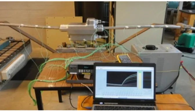
The same sensor has been installed in a lab on a 2 m long HTLS conductor (Fig. 3). Temperatures were measured outside (far from the sensor) and inside of the sensor (on the conductor surface), on the clamps between conductor and sensor, as well as on the wall surface of the sensor. (Abscissa zero being located on the conductor surface in the middle of sensor).

Fig. 3 General view of thermal test‟s setup

For the application, the clamp is different at the two ends of the sensor: one is made of elastomer material, the other is metallic (aluminium).

Special attention was dedicated to maintain the current flow constant, as conductor resistance was fluctuating with temperature.

III. TESTCAMPAIGN

Temperature, current flow and voltage were recorded every minute with a Fluke Hydra temperature logger. Sensor was installed between abscissa -18.5 cm and 18.5 cm.

A. Without Wind

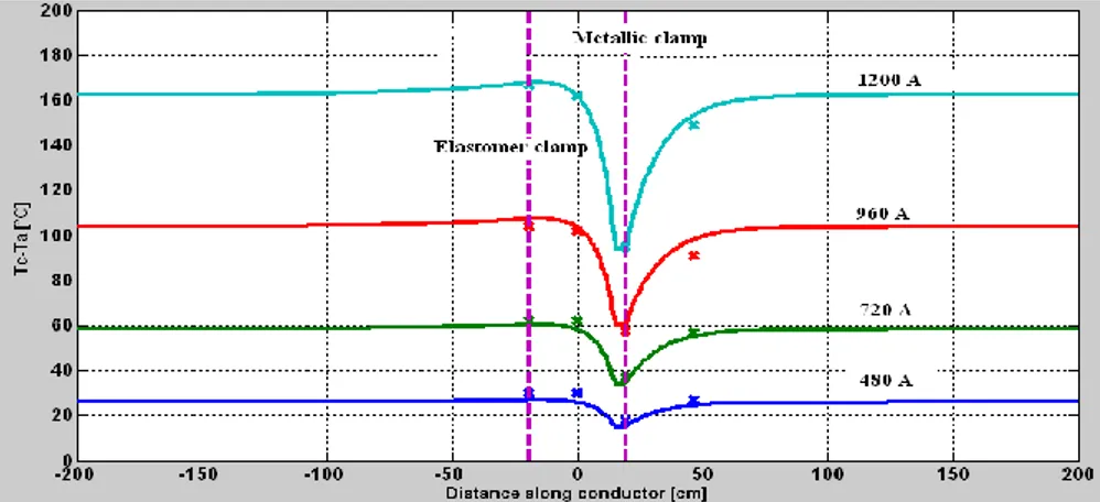
Table 1 and Figure 4 show the lab test results without the sensor installed.

It can be seen in Figure 4 that temperature obviously varies little along the conductor; for each current, the average measured conductor temperature (Tc-Ta) is compared with calculation (detailed later on) as shown in Table 1.

TABLE1THEMEASUREDANDCALCULATEDCONDUCTORTEMPERATURES(SEE§IV&V)OVERAMBIENTATEQUILIBRIUMATNO

WIND(AMBIENT20°C),NOSUN(NOSENSORINSTALLED)

Current flow(A) Measured (Tc –Ta) (°C) Calculated (Tc–Ta) (°C)

480 30.8 ± 1.7 28

600 45 ± 3 46.7

840 84 ± 4.7 84

960 111.5 ± 3.5 113

1200 162 ± 4 159

Fig. 4 Measured and calculated equilibrium temperatures increase (over ambient) on the HTLS conductor surface along the sample at no wind, no sun (No sensor installed) (Ambient near 20°C)

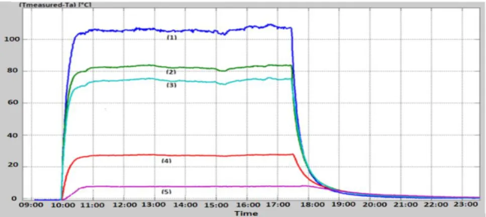
The Figure 5 shows the lab test with the sensor installed, at no wind and 1200 A applied during about 6 hours. Different transients can be seen in and out of the sensor.

Fig. 5 Transient time evolution (12 hours) of several temperatures increase (over ambient) at no wind no sun conditions (1200A)

Once the sensor is installed, many transients have been recorded at different locations. Each has its own time constant, as detailed in Table 2. Obviously conductor has now reach different temperatures depending on location, the sensor acting as a heat sink.

TABLE2RELATIVEINCREASEOFCONDUCTORTEMPERATURESOVERAMBIENTATEQUILIBRIUM(TIMECONSTANT)ATNOWIND

(AMBIENT20°C),NOSUN(SENSORINSTALLED)

Current flow (A)

Conductor at distance of 20cm from metallic clamp

Conductor

inside sensor Metallic clamp Elastomer clamp

480 27°C (20‟) 30°C (28‟) 18°C (50‟) 30°C (26„)

720 57°C (21‟) 62°C (30‟) 37°C (51‟) 62°C (28„)

960 91°C (17‟) 102°C (34‟) 58°C (40‟) 104°C (26„)

1200 149°C (18‟) 162°C (25‟) 95°C (37‟) 167°C (24„)

1: conductor temperature in contact with elastomer clamp, 2: conductor temperature in the middle of sensor, 3: conductor temperature out of sensor, 4: conductor temperature in contact with metallic clamp, 5: temperature of sensor‟s external surface. B. With Wind

The next Figures 6 and 7 show similar outputs as before, with the action of wind speed. The global data from those tests are summarised in the Table 3:

TABLE3CONDUCTORTEMPERATURESINCREASEOVERAMBIENT(TIMECONSTANT)ATPERPENDICULARWINDSPEEDMAX3M/S

ACTINGONTHESENSOR(AMBIENT20°C),NOSUN

Current flow(A) Conductor at a distance of 20cm from metallic clamp

Conductor

inside sensor Metallic clamp Elastomer clamp

720 40°C (14‟) 30°C (11‟) 10°C (16‟) 26°C (13„)

960 61°C (12‟) 51°C (10‟) 17°C (11‟) 45°C (10„)

1200 105°C (10‟) 83°C (9‟) 27°C (13‟) 74°C (9„)

Wind was created with a local electric fan and thus had a wind profile not constant but reproduced in the Figure 6.

Fig. 7 The same as Fig. 5 but with acting wind (3m/s), 1: conductor temperature out of sensor, 2: conductor temperature in the middle of sensor, 3: conductor temperature in contact with elastomer clamp, 4: conductor temperature in contact with metallic clamp, 5: temperature of sensor‟s external surface

It must be emphasized that the highest temperature is now observed on the conductor in the free span (far from the sensor). IV. THERMALMODEL

A sophisticated model would be of no hope in such problem. Indeed every detail of the sensor has its own influence and external wind, sun, rain, etc. would also affect the outputs. Only a global overview may be reached and may be of practical interest for engineers.

In general, a model is a representation of reality that retains its salient features. To estimate the mathematical model describing the longitudinal variation of conductor temperature with sensor installed, we first have to identify and analyse the system under study.

Given the high thermal heterogeneity of the system proved previously by the measurements, and its regular geometry, we can split the analysis into two kinds of zone (out of the sensor and inside the sensor) with particular boundary conditions in between. Each zone is characterized by its heat transfer mode. If far outside the sensor, only convection and radiation occur (no longitudinal conduction). Longitudinal conduction cannot be neglected close to boundary conditions (especially metallic clamp) as well as inside the sensor due to heat sink effect of the metallic mass and surface of the sensor itself which drains calories from the conductor to the sensor box to heat it up and evacuate them to the ambient (Fig. 8).

Fig. 8 The thermal model of axial temperature variation along the conductor with sensor installed

In general, any metal piece installed on the conductor has the potential to cause a heat sink; the added surface area of the sensor increases the convection and radiation losses, which tends to reduce the local temperature compared to undisturbed conductor.

For the model, clamps are area from where heat can be extracted if conductivity is large enough (which is not the case if the clamp is made of elastomer) and if the connected extra surface (the sensor) is significant compared to the conductor surface under the clamp.

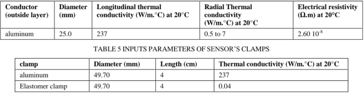
TABLE4SOMEOFTHEOUTSIDELAYERCONDUCTORPROPERTIES Conductor (outside layer) Diameter (mm) Longitudinal thermal conductivity (W/m.°C) at 20°C Radial Thermal conductivity (W/m.°C) at 20°C Electrical resistivity (Ω.m) at 20°C aluminum 25.0 237 0.5 to 7 2.60 10-8

TABLE5INPUTSPARAMETERSOFSENSOR‟SCLAMPS

clamp Diameter (mm) Length (cm) Thermal conductivity (W/m.°C) at 20°C

aluminum 49.70 4 237

Elastomer clamp 49.70 4 0.04

It is of prime importance to consider separately radial and longitudinal thermal conductivity. Inside a conductor (from the central part to the outside), the thermal conductivity is known by the literature [11, 12] to be quite low (about 1 W/m°C) compared to the aluminum property (237 W/m°C). That is due to the air encapsulated between the strands. Such data is the key factor to evaluate temperature gradient from the core to the surface but this is not considered here.

To evaluate longitudinal gradient (our concern), the calories will follow the individual strands of the conductor (towards the metallic clamp), thus using the full aluminum thermal conductivity. The sensor body will then dissipate a considerable amount of heat depending on its external surface open to the ambient. Similarly for transients, the mass of the sensor will also store calories and will completely modify local thermal time constant.

The sensor acts as a heat sink from few meters apart towards the sensor. All of these phenomenons will now be modeled and analyzed.

To make the thermal model as simple as possible, some assumptions have been made:

 Assumption 1: The conductor is thermally isolated from the sensor at contact with elastomeric clamp. No thermal flux could transit towards the sensor at that location. (Fig. 8)

 Assumption 2: The heat loss can be modeled linearly with a heat transfer coefficient “h” so that it can be written as: q = h. (T - Tref), Pc, r= π D q (1)

With q [W/m²] is heat flux, h [W/m² °C] is heat transfer coefficient, T [°C] is conductor temperature, and Tref [°C] is reference temperature (ambient or sensor), Pc, r [W/m] is convective (radiative) cooling, and D [m] is the conductor‟s outer diameter.

 Assumption 3: The sensor‟s external surface is isothermal; the flux is transmitted from the conductor to the sensor through the metallic clamp.

 Assumption 4: We assume that we have an axial symmetry; the transfer of heat from sensor‟s external surface is therefore only radially. The sensor‟s equivalent radius Rs is set equal to 95 mm in our test.

The thermal behaviour of the conductor in unsteady state is determined by the balance between heat gains and heat losses as exposed in the following Equation 2:

2 ( )? ( ) 2 2 long av j c r Q dT D D C P P P dt x         (2)

Where, Tav [°C] is the average conductor temperature, Pj [W/m] is joule heating, Pc [W/m] is convective cooling, Pr [W/m] is radiative cooling, [kg/m³] is the mass density, C [J/Kg. °C] is the specific heat capacity, and Qlong [W/m²] is the conductive longitudinal heat flux (qcin and qcout on Fig. 8)

Fourier‟s law (Eq. 3) defines the heat flux emitted by conduction into the conductor (longitudinal):

long T Q K x     (3)

With K [W/m °C] is conductor‟s thermal conductivity (See Table 4), and T

x 

 [°C/m] is the temperature gradient.

V. STEADYSTATEANALYSIS

In order to examine the conductor‟s thermal behaviour in steady state with sensor installed, under controlled environmental conditions, the heat balance (Eq. 2) was simplified by taking into account the previous assumptions. Therefore, the generalized balance equations (Eqs. 4, 6) for each block of conductor looks like:

For conductor outside of sensor (No Sun): 2 T 4 (T ) 0 ² ( )? 2 J a out out a P h T K D D x        (4)

Where Tout [°C] is conductor‟s temperature outside of sensor, ha [W/m² °C] is the heat transfer coefficient that combines convective and radiative heat losses.

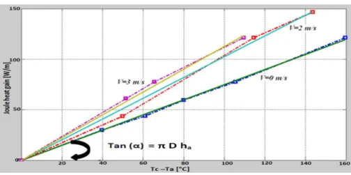
A first estimate of the analogic expression of ha [W/m² °C] can be derived from a month of measurements as follows (Fig. 9): 0.54 1 [0.3674 24.8 5.9( . ( ) ] a h D DV x D      (5)

Where V(x) [m/s] is the wind speed along conductor, ε is the conductor‟s emissivity;

Fig. 9 The fit of the heat transfer coefficient (π D ha) according to measurements

After determining the heat transfer coefficient ha for each wind speed through the measurements, a fit of type a+b VC is applied to describe the heat transfer coefficient with wind (Eq. 5).

The term of24.8 D (Eq. 5) is obtained by the linearization of Stephan Boltzmann equation used to compute the radiative cooling.

For conductor inside of sensor:

This is obviously sensor dependent; the sensor is defined here by two parameters, its global convective surface and its conductive length in contact with the conductor: Lcm (Fig. 8).

The metallic clamp is supposed cylindrical with an inner radius equal to conductor radius R, and external radius Rcm (Table 5). 2 ² 4 ( ) 0 ² ( ) 2 J b in in s P h T T T K D D x        (6)

Where Tin [°C] is conductor‟s temperature inside of sensor, Ts [°C] is temperature of sensor‟s external surface (isothermal area), and hb [W/m² °C] is the heat transfer coefficient due to convection.

Similar to the heat transfer coefficient ha, the heat transfer coefficient hb [W/m² °C] (Eq. 7) is modeled as follows (figure not drawn but similar in its shape as Fig. 9):

0.70 1 [0.6490 4.46( . ( ) ] b h DV x D    (7)

The radiative cooling inside the sensor is neglected (<10-5 W/m).

The global model

Hence the studied system (conductor + sensor) is described by two partial differential equations of second order (Eqs. 4, 6); their solutions are determined using the following boundary conditions (Eqs. 8, 9, and 10):

1: at metallic clamp: The metallic clamp may be considered as a cooling radial fin that increases the rate of heat transfer from the conductor, to the sensor‟s surface, towards the environment of temperature Ta. The extracted heat can be expressed as:

cm cm cm a

q h (T T ) (8)

Where:

 qcm [W/m²] is the heat transfer rate across metallic clamp, Tcm [°C] is conductor‟s temperature in contact with metallic clamp, hcm [W/m² °C] is the coefficient of radial heat conduction across the metallic clamp:

s s s cm 1 cm 1 cm 1 cm s 0 1 cm cm cm s cm 0 1 cm 1 cm 0 s 0 0 cm S S [h . K .c.I (c.R )].K (c.R) [K .c.K (c.R ) h . .K (c.R)].I (cR) S S K .c. S K .c.[K (c.R).I (c.R ) K (c.R ) I (c.R)] h . .K (c.R).[1 I (c.R)] S       With:

 Kcm [W/m °C] is metallic clamp‟s thermal conductivity (Table 5), 2 a cm cm

2.h c

L .K

 ,

 I0 (I1) and K0 (K1) are modified Bessel functions of order zero (of order one), of first and second kind, respectively,  Scm [m²] is the metallic clamp surface, Ss [m²] is sensor‟s surface.

 The heat transfer coefficient hs [W/m² °C], due to convection and radiation between sensor‟s external surface and ambient is modeled from a month of measurements (the same manner as ha) as follows:

1.11 s s s s s 1 h (2.05 40.83. .R 31.8071(R .V(x) ) 2 R     

Where V(x) [m/s] is the wind speed along the sensor, and Rs [m] is the equivalent sensor‟s radius, s is the sensor‟s emissivity.

2: at elastomer clamp: The conductor is thermally isolated (Assumption 1): ce

q 0 (9)

Where qce [W/m²] is the heat transfer rate across elastomer clamp

3: When x tends to infinity, conductor temperature is uniform. There is no lateral conduction flux and the equation (Eq 4) can be solved as follows:

2 a inf a a I S T T .D.h     (10)

Where ρa [Ω.m] is the resistivity of the conductor at 20°C, I [A] is the total current, and S [m²] the conductive cross-sectional area.

Once we have properly posed the problem, the available analytic solutions of the heat equations (Eqs. 4, 6), considering the boundary conditions (Eqs. 8, 9, 10), define the temperature profile along the conductor as detailed on Eqs. 11, 12 and 13 and as shown on following Figures 10 (without wind) and 11 (with wind).

Inside of sensor: J in s 1 2 b b b P x x T (x) T A .exp( ) A .exp( ) d d .D.h       (11) With s 1 b L A Y exp( ) 2d    s 2 b L A Y exp( ) 2d  

Outside of sensor (near elastomer clamp):

ce inf outL inf s a a T T x T (x) T exp( ) L d exp( ) 2.d     (12)

inf cm outR inf s a a T T x T (x) T exp( ) L d exp( ) 2.d      (13)

Where, Ls[m]is the length of sensor (about 35 cm); Tcm [°C] and Tce [°C] are respectively the temperature of conductor in contact with metallic clamp (elastomer clamp), And y, db, and da, are detailed as follows:

j cm b s s cm cm b b b b P h .D.h Y L K L K [exp( )( h ) exp( )( h )] d d d d        , b b K.D d 4.h  , a a K.D d 4.h 

Figs. 10 (without wind) and 11 (with wind) can be drawn using these equations. They give access to the temperature profile along the conductor with sensor installed.

Fig. 10 The temperature profile along conductor according to simplified thermal model, compared with measurements (cross x), sensor installed, no wind, no sun (Heat sink of 65°C, at metallic clamp with a current of 1200 A)

Fig. 11 The same as Fig. 10, with a max 3 m/s wind speed perpendicular to the conductor but localized as shown on Fig. 6 (Heat sink of 130°C, at metallic clamp with a current of 1200 A)

The temperature profile at the output of the elastomer clamp, inside the sensor has a zero derivative, corresponding to local boundary conditions of qce=0 (Assumption 1) towards the sensor.

Some specific calculated temperatures are shown in Table 6 (no wind), and Table 7 (with wind):

TABLE6RELATIVEINCREASEOFCONDUCTORTEMPERATUREOVERAMBIENTATEQUILIBRIUMACCORDINGTOSIMPLIFIED

THERMALMODELATNOWIND(AMBIENT20°C)NOSUN(SENSORINSTALLED)(TOBECOMPAREDWITHTABLE2FORMEASURED

VALUES)

Current flow(A) Conductor at a distance of 20 cm from metallic clamp

Conductor inside sensor

Metallic clamp Elastomer clamp

480 25°C 29°C 15°C 27°C

720 55°C 59°C 34°C 60°C

960 96°C 103°C 60°C 107°C

TABLE7CONDUCTORTEMPERATUREINCREASEOVERAMBIENTATEQUILIBRIUMACCORDINGTOSIMPLIFIEDTHERMALMODEL

WITHAPERPENDICULARWINDSPEEDMAX3M/SACTINGONTHESENSOR(AMBIENT20°C)NOSUN(TOBECOMPAREDWITHTABLE3

FORMEASUREDVALUES)

Current flow(A)

Conductor at a distance of 20 cm from metallic clamp

Conductor inside sensor Metallic clamp Elastomer clamp

720 40°C 30°C 12°C 29°C

960 64°C 48°C 20°C 49°C

1200 105°C 79°C 33°C 80°C

At the equilibrium, it is clear that the estimated temperatures from the thermal model (Tables 6, 7) proved to be reasonably close to those obtained from measurements (Tables 2, 3); the average error is of the order of 2°C, and the maximum error is about 6°C, which is admissible considering all simplified hypothesis.

The conductor‟s temperature evidently has its minimum value at the sensor‟s metallic clamp location (Figs. 10, 11) and then increase out until approximately (1 m-1.5 m).

During windy conditions, the zone of sensor effect can reach 3 m on both sides. VI. TRANSIENTSTATEANALYSIS

In transient state, the temperature of an overhead power conductor is constantly changing in response to changes in electrical current and weather conditions; indeed, for a step change in electrical current (as shown in Figs. 5 and 7 during our tests), the conductor temperature (solution of Equation 2) can be expressed by (Eq. 14):

t

c i f i

T (t)T (T T )(1 e ) ₍₁₄₎

Where Tf [°C] is steady state conductor temperature and Ti [°C] is the initial conductor temperature. The conductor heating time constant is deduced from Eq. 2 as:

c

m .C .D.h  

 (15)

Where m [kg/m] is conductor mass per unit length, C [J/Kg.°C] is the conductor specific heat capacity (about 897 J/Kg.°C at 20°C, and quasi constant with temperature in our range of test), and his the heat transfer coefficient (ha: out of sensor and hb inside of sensor).

In those ranges, the influence of the load current is low. At the metallic clamp, the system time constant is calculated as:

S

S S

m .C S h

  (16)

Where ms [kg] refer to the mass of sensor (about 6 kg in our test).

The system‟s time constant says that large mass and large specific heat capacity lead to slower changes in temperature while large surface and better heat coefficient (high wind speed) lead to faster temperature changes. This relationship helps to design the sensor by reducing its mass and maximizing its surface area.

Table 8 is giving experimental vs. computed time constants as follows:

TABLE8CALCULATEDTIMECONSTANT(DEVIATIONBETWEENCALCULATIONANDMEANMEASUREDTIMECONSTANTSFOREACH

ZONE),WITHANDWITHOUTWIND(AMBIENT20°C),NOSUN(SENSORINSTALLED)

Wind speed (m/s)

Conductor at a distance of 20 cm from metallic clamp

Conductor

inside sensor Metallic clamp

Elastomer clamp

0 29‟ (53%) 30‟ (2%) 51‟ (15%) -

3 11‟ (-8%) 14‟ (40%) 19‟ (36%) -

It has been shown through calculation that estimated time constants present admissible agreement with experimentation. VII. THESAMEMODELAPPLIEDONANOTHERCONDUCTOR

To test our model sensitivity to input parameters, the developed thermal model (same previous coefficients ha, hb, hs, and hcm) was tested using an AAAC conductor with the following properties (Table 9):

TABLE9AAACCONDUCTORPROPERTIES conducto r outside diameter (mm) Emissivity Longitudinal thermal conductivity (W/m °C) Radial thermal Conductivity (W/m °C) at 20°C Electrical resistance (Ω/m) at 20°C AAAC 30 0.7 237. 0.5-7 3.74 10-5

The same experimental procedure was used in the previous laboratory tests (See § II, III) and that without wind. Figure 12 shows the results of these experiments vs. calculation:

Fig. 12 The temperature profile along AAAC conductor according to simplified thermal model, compared with measurements, sensor installed, no wind, no sun

This test shows that even using a different conductor, but using the same formulation for h coefficients, the thermal model gives satisfactory results compared to the measurements. The error reaches 7°C on maximum with a current of 950 A.

VIII. SOMEGLOBALOBSERVATIONS  It can be noticed that sensor‟s zone effect exceeds several meters of each side.

 The measured sensor temperature differs from the conductor temperature in the free span. This is due to the higher convective surface regarding thermal flow: local conductive material is a heat sink. It is frequently the case when spacers, slices, clamps are installed on power lines.

 We have qualified and quantified such effect for conductor temperature up to 200°C (as used with HTLS) with lab test confrontation on both static and dynamic action:

 Heat sink local effect was measured up to 130°C at 1200 A on a HTLS (conductor in free field being at about 160°C over ambient when conductor at metallic clamp would be at 30°C over ambient)! Moreover, such effect is very much wind dependent. Heat sink is going from 65°C at no wind, up to 130°C at only 3m/s wind speed.

 The transient time (roughly speaking 3 times the time constant or near 2 hours at no wind, near the metallic mass) to reach the steady state conductor temperature is shortened when wind speed is applied. A difference of a factor near 3 occurs between no wind and 3 m/s!

Being always in transient on the field due to varying charge and varying weather conditions, it must be extremely difficult to manage such effect inside temperature sensors to give appropriate conductor temperature needed to evaluate the rating of the line.

In order to ensure reliable results, care must be exercised in selecting type and number of sensor to be used and the location where they are to be installed.

Even without heat sink effects, the large variability of the temperature along the ruling span indicates that adequate determination of the conductor‟s average temperature would require at least 5-8 sensors distributed along the ruling span [13].

IX. CONCLUSION

Sensors (or any metallic pieces) are influencing drastically local conductor temperature of power lines.

Despite its positive impact on conductor ageing, a reverse model (from measured local temperature inside a sensor to outside free field conductor temperature) may be hardly developed as wind speed drastically influences the outputs.

In general local wind speed acting on the sensor is unknown and may be quite different from the wind speed along the span which makes very difficult the extrapolation of mean temperature along the span, the data which has to be considered for

power line dynamic rating.

The impact zone of sensor is depending on their characteristics (mass, surface, clamps material and contact lengths) and may be extended over several meters apart depending on wind speed.

The impact zone of sensor also increases with current flow into the conductor. REFERENCES

[1] Vincent T. Morgan. “Thermal behaviour of electrical conductors. Steady, dynamic and fault-current ratings”. RSP Press, Taunton, England. 1991.

[2] Kiessling F., Nefzger P., Nolasco J.F., and Kaintzyk U. 2003. “Overhead power lines. Planning, design and construction”. Springer, Berlin.

[3] A. Deb. “Power line ampacity system.” 2000. CRC Press, p. 251.

[4] “Thermal behaviour of overhead conductors”. 2002. Cigre Technical Brochure No. 207. Study Committee B2.

[5] “Guide for selection of weather parameters for bare overhead conductor ratings.” 2006. Cigre Technical Brochure No. 299. Study Committee B2.

[6] “Sag-tension calculation methods for overhead lines.” 2007. Cigre Technical Brochure No. 324. Study Committee B2. [7] “Guide for application of direct real-time monitoring systems.” 2012. Cigre Technical Brochure No. 498. Study Committee B2. [8] IEEE Standard 738-2006. “IEEE Standard for calculating the Current-temperature of bare overhead conductors”. IEEE Power

Engineering Society. 2006.

[9] Aluminium association handbook, 2nd Edition, 1981.

[10] V.T. Morgan. “The loss of tensile strength of hard-drawn conductors by annealing in service”. IEEE Trans on PAS, vol. PAS-98, iss. 3, 1979.

[11] B.Clairmont, D.A.Douglass, J.Iglesias, and Z.Peter. “Radial and longitudinal temperature gradients in bare stranded conductors with high current densities”, CIGRE 2012, B2-108.

[12] “Theoretical model for temperature gradients within bare overhead conductors”, IEEE Transactions on Power Delivery, vol. 3, iss. 2, April 1988.

[13] Tapani O. Seppa, Robert D. Mohr, and John Stovall. “Error sources of real-time ratings based on conductor temperature measurements”, Report to CIGRE WG B2.36 (Guide on direct real time rating systems) Stockholm, Sweden, May 20-21, 2010.

[14] Morgan, V. T., Effect of Elevated Temperature Operation on the Tensile Strength of Overhead Conductors, IEEE Paper 95 WM 229-5 PWRD, IEEE/PES Winter Power Meeting, 1995.

[15] Black, W. Z. and Byrd, W. R., “Real-time Ampacity model for overhead lines,” IEEE Transactions on Power Apparatus and Systems, vol. PAS-102, iss. 7, July 1983, pp. 2289-2293.

[16] Foss, S.D., Lin, S.H., and Fernandez, R.A., “Dynamic thermal line ratings- Part 1-Dynamic ampacity rating algorithm.” IEEE Transaction on Power Apparatus and Systems, vol. PAS-102, iss. 6, pp. 1858-1864, June 1983.

[17] T. O. Seppa, “Accurate Ampacity determination; Temperature-Sag Model for Operational Real time Ratings”, IEEE Transactions on Power Delivery, vol. 10, iss. 3, pp. 1460-1470, July 1995.

[18] J. L. Lilien, E. Cloet, and P. Ferrieres, “Experiences of French TSOs using AMPACIMON real-time dynamic rating system”. CIGRE 2010, CIGRE session papers, Group C2.

Salima Balghouzal received her degree in electrical engineering from the national school of applied sciences (ENSA), University of cadi Ayyad (Morocco) in 2010. She is now a PhD student at the University of Liège (Dept. Electricity, Electronics and Computer Sciences, Unit of Transmission and Distribution of Electrical Energy).

Professor J. L. Lilien, PhD., is the head of the unit Transmission and Distribution of Electrical Energy at the Montefiore Institute of Technology, University of Liège, Belgium. He has over 30 years experience solving the electrical and mechanical engineering problems of power systems. His work involves analysis of problems in “cable dynamics” in general and on overhead power lines in particular.

His major activities were devoted to (i) vibrations on transmission lines, in particular galloping, including its control (ii) large movements of cables, like short-circuit (both in substations and power lines), (iii) health monitoring of power lines (sag and vibrations) and last, but not least (iv) low-frequency electric and magnetic field effects on human beings.

Jean-Louis is a long-time active member of IEEE and CIGRE, where he has served as convenor of several task forces of CIGRE study committee B2, “overhead lines” and B3 “substations”.

He has published over 100 technical papers in peer reviewed publications. He is the initiator and organizer from 1995, of the CABLE DYNAMICS conference.

Professor Mustapha El Adnani, Dr, Ir. received his PhD degree in electromechanical engineering in 1987 at the University of Liège (Belgium). His main research activities are on power systems design, like large movements of cables (short-circuit). His recent interest is focused on renewable energies, monitoring and control systems with intermittent production (wind, solar).

He is actually Professor at ENSA Cadi Ayyad University, Marrakech, Morocco. Mustapha El Adnani is the director and founder of the engineering school in Marrakech; he is vice president of RMEI (Mediterranean Engineering School Network).