- - - -- - -
-UNIVERSITÉ DU QUÉBEC À MONTRÉAL
PARKING PRICES AND URBAN SPRA WL IN CANADIAN METROPOLIT AN ARE AS
THESIS PRESENTED
AS A PARTIAL REQUIREMENT OF THE MASTER OF URBAN STUDIES
BY
MISCHA YOUNG
Avertissement
La diffusion de ce mémoire se fait dans le respect des droits de son auteur, qui a signé le formulaire Autorisation de reproduire et de diffuser un travail de recherche de cycles supérieurs (SDU-522 - Rév.O? -2011). Cette autorisation stipule que «conformément à l'article 11 du Règlement no 8 des études de cycles supérieurs, [l'auteur] concède à l'Université du Québec à Montréal une licence non exclusive d'utilisation et de publication de la totalité ou d'une partie importante de [son] travail de recherche pour des fins pédagogiques et non commerciales. Plus précisément, [l'auteur] autorise l'Université du Québec à Montréal à reproduire, diffuser, prêter, distribuer ou vendre des copies de [son] travail de recherche à des fins non commerciales sur quelque support que ce soit, y compris l'Internet. Cette licence et cette autorisation n'entraînent pas une renonciation de [la] part [de l'auteur] à [ses] droits moraux ni à [ses] droits de propriété intellectuelle. Sauf entente contraire, [l'auteur] conserve la liberté de diffuser et de commercialiser ou non ce travail dont [il] possède un exemplaire.»
UNIVERSITÉ DU QUÉBEC À MONTRÉAL
LES COÛTS DE TRANSPORT ET LEURS EFFETS SUR L'ÉTALEMENT URBAIN AU CANADA
MÉMOIRE PRÉSENTÉ
COMME EXIGENCE PARTIELLE DE LA MAÎTRISE EN ÉTUDES URBAINES
PAR
MISCHA YOUNG
ACKNOWLEDGMENTS
This thesis becomes a reality with the help and support of many individuals. I would now like to extend my sincere gratitude to all of them.
Foremost, I would like to thank my two thesis directors, Professors Georges Tanguay and Ugo Lachapelle. Their collaborative knowledge and expetiise as well as their never-ending support are what made this research possible. Without their guidance and devotion this dissertation would never have been completed.
Statistician Jill Vandermeerschen from the University of Quebec in Montreal's Depatiment of mathematics for sharing her wisdom and technical know-how, and for assisting me with my endless statistic inquiries.
My parents, Mia Webster and Leland Young, for their continuous encouragement and for helping me with the tedious editing of this thesis.
The University of Que bec in Montreal, and especially the School of Management and the Department of Urban Studies and Tourism, for providing the technical resources and financial support necessary in arder to complete this endeavour.
My thanks and appreciations also go to my ~olleagues, Matthieu Caron, Didier Marquis and Étienne Pinard, for the many laughs and shared coffees, and for making this research project enjoyable at1d/or more bearable.
And fmally, I would like to extend my heartiest gratitude to my grat1dparents, who served as an inspiration in pursuing this exciting undertaking.
PREFACE
This dissertation is presented in the fon11 of a thesis by publication. As a result, the fourth chapter of this research comprises an at1icle that is currently being peer reviewed for publication in the journal Research in Transportation Economies.
1t is worth noting that as the article is an abbreviated version of the dissertation, the content preceding the article will at times be repeated in lesser detail in the article itself.
TABLE OF CONTENTS
LIST OF FIGURES ... viiii
LIST OF TABLES ... ix
LIST OF ABBREVIATIONS, ACRONYMS AND VARIABLES ... x
RÉSUMÉ ... xi
ABSTRACT ... xii
INTRODUCTION ... 1
CHAPTERI THE CONCEPT OF URBAN SPRA WL ... 6
1.1 Shaping Urban Sprawl ... 6
1.2 Defining Urban Sprawl ... 8
1.3 Measuring Urban Sprawl ... 9 1.3.1 Centrality ... 10 1. 3.2 Clustering ... 11 1.3.3 Concentration ... 11 1.3.4 Continuity ... 12 1.3 .5 Density ... 12 1.3.6 Mixed Uses ... 13 1.3. 7 Nuclearity ... 14 1.3.8 Proximity ... : ... 14 CHAPTERII LITERA TURE REVIEW ... 15 2.1 The Causes ofUrban Sprawl.. ... 15
2.2 Transportation Costs ... 21
2.3 Parking Priees ... 22
CHAPTERIII DATA AND METHODOLOGY ... 26
vi
3.1 Introduction ... 26
3.2 Theoretical Scheme and Fran1ework ... 26
3.3 Description of Case Study ... 29
3.4 Data Description ... ·.··· ... 32 3. 5 Dependent Variables ... 3 2 3.5.1 Density ... 33 3.5.2 Proxinlity ... 33 3.6 Independent Variables ... 34 3.6.1 Gasoline Priee ... 34 3.6.2 Parking Priees ... 36 3.6.3 Population ... 38
3.6.4 Agricultural Land rent.. ... 39
3.6.5 Household Inco1ne ... 39 3.7 Descriptive Statistics ... 40 3.8 Econometrie Model ... .-... 45 3.8.1 Estimation Strategy ... 45 CHAPTERIV ARTICLE ... 48 4.1 Introduction ... 50
4.2 Urban Sprawl and the Natural Evolution Theory ... 51
4.3 Transportation Costs ... 54 4.3 .1 Parking Priees ... 55 4.4 Methodology ... 57 4.4.1 Data ... 57 4.4.2 Dependent variables ... 59 4.4.3. Independent variables ... 60 4.4.4. Descriptive Statistics ... 62 4.4.5 Econometrie Mode! ... 66 4.5 Results ... 68
4.5.1 Dependent Variable: Density (Proportion of Low-Density Housing) ... 68
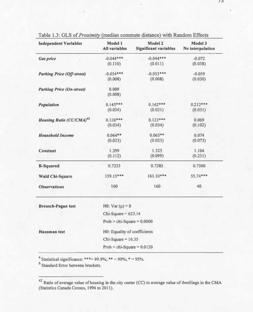
4.5.2 Dependent Variable: Proximity (Median commuting distance) ... 71
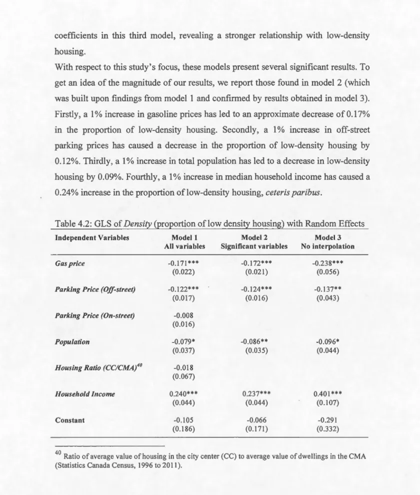
4.6 Discussion ... 74
4.7 Conclusion ... 77
CHAPTER V DISCUSSION AND ANAL YSIS ... 79
5.1 Discussion and Statistical Inference ... 79
CONCLUSION ... 84
APPENDIXA INDEPENDENT VARIABLES ... 88
APPENDIXB STATISTIC CHARACTERISTICS AND TEST RESULTS ..... ... . 90
viii
LIST OF FIGURES
Figme Page
2.1 Property values, agriculturalland values and the city limits ... 16
2.2 Decrease in transportation costs, property values and the city limits ... 17
3.1 Theoretical framework ... 28 3.2 10 Canadian CMAs included in the study ... 31
3.3 Real gas priees in Canadian cities ... 35
3.4 Off-street parking priees in Canadian cities ... 3 7 3.5 On-street parking priees in Canadian cities ... 38
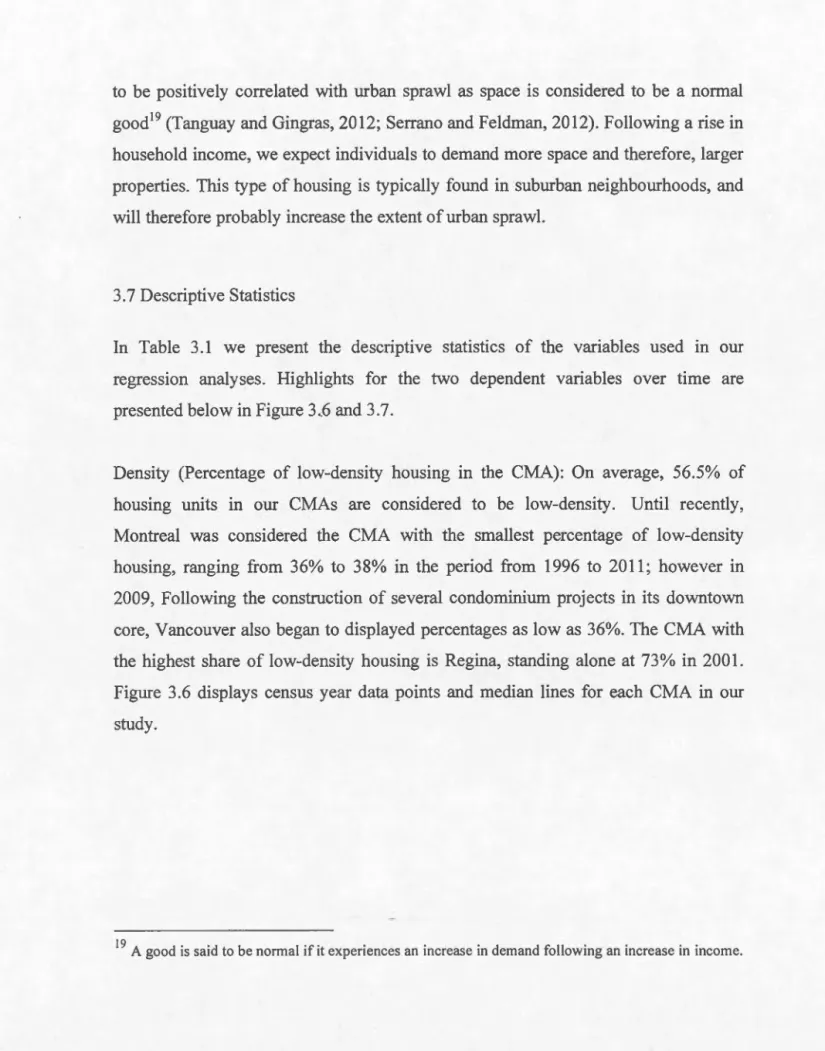
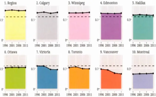
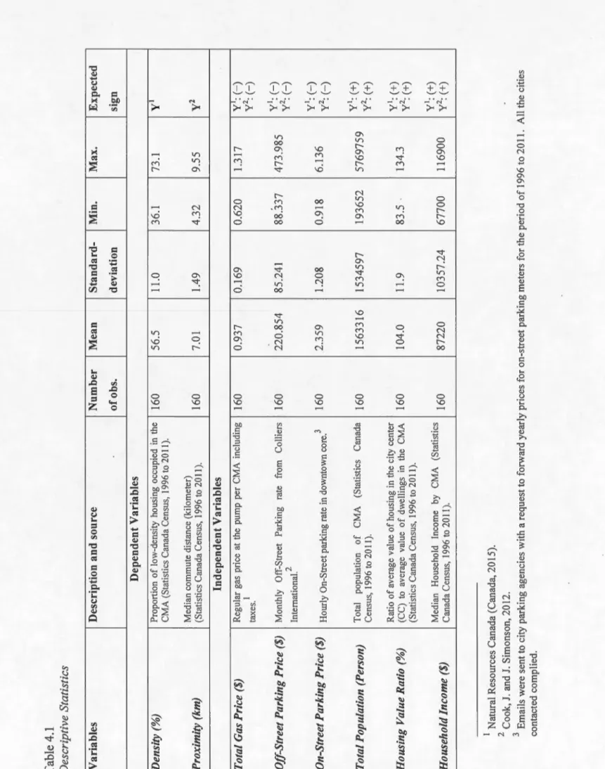
3.6 Density: proportion oflow-density housing in Canadian cities ... .41
3.7 Proximity: median commute distance in Canadian cities ... .42
4.1 Property values, agriculturalland values and the city limits ... 53
4.2 Proportion of low-density housing in Canadian cities ... 63 4.3 Median conunute distance in Canadian cities ... 64
LIST OF TABLES
Table Page
3.1 Descriptive statistics ... 44 4.1 Descriptive statistics ... 65 4.2 GLS of Density (proportion of low density housing) with Random Effects ... 70 4.3 GLS ofProximity (median commuting distance) with Random Effects ... 73 5.1 Expected change in low-density housing resulting from a 10% increase
in statistically significant independent variables ... 81 5.2 Expected change in median commute distance resulting from a 10%
- - - --
-x
LIST OF ABBREVIATIONS, ACRONYMS AND VARIABLES
CBD
cc
CPI CMA GES GHG GLS OPECCentral Business District City Center
Consumer Priee Index Census Metropolitan Area Gaz à Effet de Serre Greenhouse Gases
Generalized Least Squares Regression
Organization of the Petroleum Exporting Countries Agricultural Rent
Land Rent
Intercept of Agricultural Rent and Land Rent
New Intercept of AgricuJtural Rent and Land Rent following a Decrease in Transportation Costs
RÉSUMÉ
L'étalement des villes en Amérique du Nord constitue une problématique importante pom les gouvernements en raison de ses multiples implications économiques et environnementales. Le développement urbain en périphérie des villes accroît notamment les coûts reliés aux infrastructures d'eau et de transport, en plus de restreindre l'efficacité du transport collectif et de contribuer à l'augmentation des gaz à effet de serre (GES). Cependant, plusieurs causes de ce phénomène sont souvent débattues dans la littérature scientifique et demetuent à étudier.
Notre article vise à déterminer les effets des coûts de transport sur l'étalement urbain. Pour ce faire, nous utilisons des données provenant de 10 régions métropolitaines canadiennes pour la période de 1996-2011 et procédons à une analyse de régression afin de tester le modèle d'évolution natw·elle de Mieszkowki et Mills. En incluant des variables de contrôle comme le revenu, la population, et la valeur des terres agricoles, nous isolons l'effet qu'ont les coûts de l'essence et du stationnement sur l'étalement des villes. Deux mesures d'étalement seront utilisées dans notre recherche : la densité et la proximité. Nos résultats indiquent que des hausses des coûts de transport contribuent à ralentir l'étalement urbain. Cependant, ils demeurent insuffisants pour contrôler l'étendue des villes. Ceci étant dit, en établissant la relation entre les coûts de transport et l'étalement urbain, nous offrons une valable opportunité aux représentants gouvernementaux de restreindre ce phénomène.
Mots-clés: Étalement urbain, regwns métropolitaines canadiennes, pnx du stationnement, prix de l'essence, coûts de transport
xii
ABSTRACT
Given that urban sprawl discourages effective public transportation, increases road
and water infrastructure costs, and contributes to increases in greenhouse gas emissions (GHG) through greater vehicle miles travelled, the need to better comprehend this phenomenon and the factors that cause its growth are of paramount importance.
The objective of our research is to determine the potential effect of gasoline and parking priees on urban sprawl using data from ten Canadian metropolitan areas from
1996 to 2011. General Least Square regressions are used to test Mieszkowski and
Mills' natural evolution model, which claims that four variables explain urban sprawl: population growth, median household income, the cost ·of surrow1ding agricultural land and transportation costs. Two measures of urban sprawl are assessed: density and proximity. Our results indicate that increasing transportation costs do have a negative effect on urban sprawl, and more precisely, that gasoline
priees have a stronger effect than parking priees. However both these effects may not, by themselves, suffice to control sprawling cities. This being said, the presence of a relationship between transportation costs and urban sprawl provides a potentially
valuable opportunity for policy-makers to manage sprawl.
Key words: Urban sprawl, Canadian metropolitan areas, parking priees, gasoline
INTRODUCTION
Many contemporary urban development patterns found in North American cities are referred to as urban sprawl. These patterns are characterized by sorne degree of population and employment growth stagnation in established city centers while population tends to increases in surrounding peripheral regions, which themselves spread over broader areas. Evidence of this form of urban decentralization can be seen across the United States, where between 1950 and 1990, the proportion of metropolitan residents living in city centers decreased from 57% to 37% (Mieszkowski and Mills, 1993). Employment also followed ·suit as the proportion of jobs found in city centers went from 70% to 45% for that san1e time period. In their work, Glaeser and Kahn (200 1) discuss the significant decrease in employment rates felt in city centers and predict that in following decades employment in central cities across North America will rarely comprise more than 20% of the total share of employment. This trend is also noticeable in Canada where between 2006 and 2010, population growth rates in suburban communities (8.3%) surpassed population growth rates of city centers (5.3%). In fact, during this same time period, Canadian peripheries of urban agglomerations registered soaring population growth rates of up to 50% in comparison with the country's total population growth rate of 5.9% (Turcotte, 2008). People now work and live in the suburbs: "in 1960 fewer Americans lived in suburbs than in central cities or the countryside. Ten years later the suburbs had overhauled both; by 2000 they contained more people than cities and cow1tryside put together" (The Economist, 2008).
These numbers clearly illustrate the current trends taking place across North American cities, but do not explain the reasons behind these new tendencies. lt is this aspect that will be further discussed in our research in which we will attempt to better
2
understand the mam causes of urban sprawl and especially grasp the effects of transportation costs.
A number of prevwus studies have sought to identify the causes of urban sprawl. Many (Brueckner, 1987; Burchfield et al. 2006; McGibany, 2004; McGrath, 2005; Mieszkowski and Mills, 1993; Nechyba and Walsh, 2004; Song and Zenou, 2006; Tanguay and Gingras, 2012; Wassmer, 2008) have tried to explain this contemporary form of planning by using the monocentric model developed by Alonso (1964), Mills (1967), and Muth (1969). In its rudimentary form, this mathematical model suggests that a household' s housing costs will decrease as it moves further away from the city c~nter,. whereas its commuting expenses and transportation costs will increase. Using this mode!, authors have considered a range of different factors to better comprehend the determinants of urban sprawl: i) climate and topography (Burchfield et al., 2006); ii) fiscalization of land use (Wassmer, 2002, 2006, 2008); iii) property taxes (Song and Zenou, 2006); iv) racial bias (Mieszkowski and Mills, 1993); and the most prominent factors regrouped under v) the natural evolution mode! (Brueckner and Fansler, 1983; Burchfield and al., 2006; McGibany, 2004; McGrath, 2005; Mieszkowski and Mills, 1993; Song and Zenou, 2006; Tanguay and Gingras, 2012; and Wassmer, 2002, 2006, 2008). This last mode!, coined the natural evolution mode! and often attributed to Mieszkowski and Mills, is largely based on Alonso, Muth "and Mills' monocentric approach and uses four factors to explain mban sprawl: i) population size; ii) incomes; iii) agricultural rent and iv) transportation costs.
The present study concentrates on the factors associated with the natural evolution model, and as mentioned earlier, will especially focus on the effects of transportation costs. Previous readings (McGibany, 2004; Tanguay and Gingras, 2012) and observations will help us assun1e that an increase in transportation costs such as gasoline and parking priees might potentially motivate drivers to reduce their car
usage. Furthermore, these prior readings and observations will lead us to hypothesize
that if an increase in these priees can reduee car usage, they also have the potential to
reduce urban sprawl since this concept is closely related to car usage. This second
hypothesis is only conceivable if we consider and aceept the positive relationship
between urban sprawl and car usage. 1 The novelty of this analysis lies in the central focus on transportation costs and the use of parking priee data to complement other analyses that have used gasoline priees. 2 By determining if an increase in
transportation costs may help reduce urban sprawl, this study offers an opportunity
for cities and govenm1ent officiais seeking to minimize the extent of sprawl and its
many negative externalities.
As the automobile became more and more affordable for the middle class in the second half of the 20th century, transportation costs underwent a steady and substantial reduction in the form of journey costs, or time spent traveling, as
individuals were able to travel further distances with a smaller investment of time.
Thus individuals could live further away from central business districts (CBD's), which would reduce their housing costs without significantly increasing their journey
time. This stability in travel duration over time was first empirically demonstrated by
Zahavi in 1974. Portraying distance as a function of time and speed (Distance
=
Time x Speed), Zahavi showed how under the assumption of constant journey times,an increase in travel speed could on1y result in an increase in distances traveled.
Nevertheless, the distance variable in Zahavi's equation can potentially be countered
by increases in driving costs, including congestion and tolls, as well as gasoline and
parking priees. All of these have been typically on the rise in recent decades (Kane et
al. 2015).
1
Further information in regards to this relation can be found in work by Newman and Kenworthy (1999), in which they establish the positive relationship between urban sprawl and automobile dependency and clarify the process by wh ich cities expand by continually prioritizing the automobile. 2 Consider for instance the work ofTanguay and Gingras (20 12) on the effects of gasoline priees on urban sprawl.
4
The cause of this rise in transportation costs is often attributed to an escalation in the average priee of gasoline over the years. For exarnple in real terms, gasoline priees in the United States more than doubled from $1.76 per gallon in 2002 to $3.73 per
gallon in 2012 (U.S., nergy Information Administration, 2015). Other authors have
challenged the a~1obile's assumed reduction in journey costs, demonstrating that increases in congestion levels have negatively affected travel times. The American
Federal Highway Administration, reports that congestion levels now impact over two thirds of all vehicle travels in the United States, as opposed to under one third in 1982 (Urban Transport Tax Force, 2012, p. 11). Likewise, Canada's Ecofiscal Commission
fmds th at the unpredictability and variance of travel time brought upon by congestion forces half of Montrealers to allocate upwards of 60 minutes towards getting to and from work every day (Canada's Ecofiscal Commission, 2015). A third component of transportation costs is the priee of parking. Though often neglected in transpottation
cost calculations, parking priees have been increasing for decades and are now
considered a substantial cost associated with owning a private vehicle. In downtown
Calgary for instance, on-street parking now costs $5 per hour whereas Jess than twenty years ago, it was only $2.20.3•4
These examples provide evidence of a substantial increase in transportation costs and
illustrate the potential misconception surrounding the cost effectiveness of living
further away from the CBD. The objective of this study is thus to determine whether
these increases in transportation costs have had an effect on urban sprawl in Canadian
cities. Because urban sprawl inhibits effective public transportation, increases road
and water infrastructure costs, and contribute to global warming (Wilson and
Chakraborty, 2013), the need to better comprehend this phenomenon and the factors
that cause its growth seem of pararnount impmtance.
3
Information retrieved from email conversations with Rachel Knight from the Calgwy Parking
Authority, 2014. (Rachel.Knight@calgaryparking.com) 4
To test the effects of transportation costs on urban sprawl, we base our analysis on previous work by Tanguay and Gingras (2012), who, using the natural evolution
mode!, conducted a study on the effects of gas priees on urban sprawl in Canadian cities. Their results indicated that on average, a 1% increase in the adjusted priee of gasoline caused a decrease in low-density housing units by approximately 0.60% and an increase in the population living in the inner city by 0.32%, their indicators for
urban sprawl. Similarly to Tanguay and Gingras (2012) and other studies (Burchfield
et al. 2006; Molloy and Shan, 2013; Ortufio-Padilla and Femandez-Aracil, 2013), we
perform a panel regression analysis using data from 10 Canadian metropo1itan areas over a 16-year period. We measure urban sprawl using two dependent variables:
density and proximity. Independent variables that are accounted for in our research
are income, population, dwelling values, downtown parking priees (on-street and
off-street), and gasoline priees. While our results do provide evidence of a negative relationship between transportation costs and urban sprawl in Canadian metropolitan
areas, the magnitude of this relationship is somehow weaker than initially hypothesized.
In the next chapter, we define urban sprawl, identify the hypothesized causes of urban
spraw1 and discuss the different methods used to measure its extent. We then focus on transportation costs, emphasizing the novelty and impmiance of including parking priees in urban sprawl equations. The third section will elaborate our methodology
and theoretical mode!. As this dissertation is presented in the form of a thesis by publication, we present our article comprising the results of our regressions as weil as a discussion of these results in the fowth section. A brief surnmary and other concluding remarks will comprise the final section of this paper.
- - - -- -
-6
CHAPTERI
THE CONCEPT OF URBAN SPRA WL
1.1 Shaping Urban Sprawl
Before beginning to discuss urban sprawl it is imperative to reflect on cities and address the underlining forces that shape them. Often built at the intersection of major
transportation routes, cities originally served as centers for storage, for manufacture
and most importantly for trade. They allowed surrounding farmers to process and
distribute their agricultural surpluses and were regularly founded around
marketplaces to take advantage of agglomeration economies. 5 While continuing to
facilitate trade, cities now also assume the role of communication centres and provide
fertile grounds for hun1an evolution, drawing a mixture of people, cultures, talents,
and innovations (Ellis, 2011 ).
Interestingly, the size and form of cities has also evolved through time. As noted by
Newman and Kenworthy (1999), the form of cities has largely been influenced by
transport. The fom1 of ancient cities was mostly based on walking. Restricted by the condition that destinations had to be reached in an average of half an hour or less,6 the size of walking cities rarely surpassed 5 kilometers in diameter and were characterized by high levels of population density. Over time, and with the arrivai of new technical advances, cities began to expand. The advent of trams and trains
permitted faster travel and enabled cities to accommodate more people while
5
Agglomeration economies are the benefits th at individuals or firms obtain wh en they locate near one another and are often attributed to transportation cost savings (Glaeser, 201 0).
6
Condition used by Newman and Kenworthy (1999) to incorporate the stability in travel duration
respecting the half hour travel average criteria. The form of this second type of city was mostly centered on railroads and tram routes, giving cities a spider-like appearance, and where density levels were considerably reduced. The third type of city followed the arrivai of the automobile. Arguably the greatest factor to have
influenced the shape and form of cities, the automobile enabled growth as far out as 50 kilometers in ail directions and completely changed the appearance of cities forever. Subsequently faced with greater land supply, planners began building low-density housing on cheaper land often found at the outskirts of cities and towns and paved the road for the mass development of the suburbs.
Another noteworthy factor contributing to the popularization of the suburbs was the
growing recognition of health hazards associated with excessive pollution from
heavily industrialized city centers. Indeed, by relying on fossil fuels and industries to bolster their economies, cities became notorious for providing unhealthy living
conditions. Environmental problems such as water contamination and air pollution became prominent concerns and "helped fuel the exodus from central cities, and contributed to the deconcentration of cities known as sprawl" (Frumkin et al., 2004, p. 64). This, coupled with the arrivai and popularization of the automobile, led to the
birth of the phenomenon we now refer to as urban sprawl.
In order to determine the causes of urban sprawl, it is important to first defme what we mean by urban sprawl and discuss the different dimensions that will be used to measure its extent. In this first chapter we show that there are severa! ways to define urban sprawl and an even greater number of ways to measure it, each with its own advantages and flaws.
8
1.2 Defining Urban Sprawl
The term "urban sprawl" has a variety of definitions. These definitions vary
depending on the author and the field of study in which they are employed. For
instance, some authors such as Brueckner and Fansler (1983), McGibany (2004),
Burchfield et al. (2006), and Sun et al. (2007) use s_patial featmes to define urban
sprawl, claiming it is "characterized by vigorous spatial expansion of urban areas" (Brueckner and Fansler, 1983, p. 479). They emphasize the required travel distances
and the size of urban areas: "Sprawl is often used to describe cities where people need to drive large distances to conduct their daily lives" (Burchfield et al. 2006, p. 607).
Other authors, such as Pendall (1999), Nechyba and Walsh (2004), Eidelman (2010), and Banai and DePriest (2014) rather describe urban sprawl as low-density areas:
"The lower per capita consumption of land indicates a more compact development
and less sprawl" (Banai and DePriest, 2014). They commonly use changes in population and dwelling density to measure the extent of sprawl.
A third noteworthy definition is the center-periphery opposition put forth by Bussière and Dallaire (1994), Chapain and Polèse (2000) and Bordeau-Lepage (2009). This
idea tmderlines the importance and presence of displacement of residential and commercial sites from city centers to peripheral regions: "Cities expand, with
population and employment increasing more on the periphery than in the center of the
city" (Bordeau-Lepage, 2009, p.13). Similar to this notion is the definition postulated by Wassmer (2000), in which he describes mban sprawl as "another word for a certain type of metropolitan decentralization or submbanization" and follows by
adding: "suburbanization occurs over time when a larger percentage of a metropolitan area's residential and/or business activity takes place outside of its central locations" (Wassmer, 2000, p. 2).
In his later work, Wassmer (2002) reexamines suburbanization- which he believes to be a direct substitute to urban sprawl - and explains how, according to economists, suburbanization is a process determined by household's residentiallocation decisions.
These residential location decisions are in turn determined through weighing the private benefits of a suburban, decentralized location (potentially better schools, cheaper land, newer infrastructures, etc.) against the private costs of this same suburban location (longer commute times, less walking distance amenities, etc.). If private benefits outweigh private costs, households will decide to live further away from the city center, regardless of the fact that this may not be an optimal solution given the external costs of congestion and pollution.
This array of definitions exemplifies the Jack of consensus surrounding the concept of
urban sprawl and ways to measure its extent. Each definition considers a different
aspect of this phenomenon and conveys different variables to measure its scope. As a way to solve this problem, Galster et al. (2001) created a conceptual definition of
urban sprawl based on eight aspects often associated with sprawl. This definition is the one that will be favoured in this work because it considers the possibility that
there can be different types of sprawl and because it also defines sprawl as a process
of development and believes in its constant mutation over time. Bearing in mind that our research will focus on transportation costs, let us now move to examining the numero us ways of measuring urban sprawl proposed in this conceptual definition. 7
1.3 Measuring Urban Sprawl
As mentioned earlier, there are severa! definitions of urban sprawl and because of this, there are also nun1erous ways to measure it. Galster et al. (2001) have divided
7
The applicability ofthese definitions in a Canadian context is reflected by their usage in previous
10
these measures into eight dimensions: centrality, clustering, concentration, continuity,
density, mixed uses, nuclearity, and proximity.
1.3.1 Centrality
In accordance with Bussière and Dallaire (1994 ), Gordon and Richardson ( 1996),
McDonald and McMillen (2000), Felsenstein (2002), and Nechyba and Walsh
(2004), we define centrality by the percentage of a metropolitan area's population
living in the city center. This allows us to take the relative weight of the population per urban area into consideration. This approach has previously been used in the past
(Gordon and Richardson, 1996; McDonald and McMillen, 2000; Felsenstein, 2002;
and Nechyba and Walsh, 2004) to analyze cases of decentralization in urban regions
of the Uruted States. To measure centrality, Douglas and Denton (1988) propose
using Geographie Information Systems software to draw series of concentric rings
from the city center. The cumulative population of each ring is then computed to
determine centrality.
Other authors, such as Galster et al. (2001) and Wassmer (2000, 2002), rather defme
centrality in relation to land usage, concluding that centrality is "the degree to which
observations of a given land use are located near the central business district,"
(Galster et al. 2001, p. 701) thus concluding that urban areas are decentralized when a
greater distance is required to cover the same proportion of development. It is worth
noting that measuring sizes of urban regions to better understand urban sprawl is in
no way a new approach and has been abundantly used in the past. Brueckner and
Fansler (1983), McGibany (2004), McGrath (2005), and Song and Zenou (2006), to
name a few, have used this sizing method in their econometrie models to comprehend different aspects of urban sprawl.
-1.3.2 Clustering
In order to measure urban sprawl, Gordon and Richardson (1997) have used
clustering. Clustering measures the degree to which an urban area is bunched together in order to minimize the amount of developable land need to contain residential
development. As explained by Jaeger et al. (201 0, p. 400), "the degree of urban
sprawl will depend on how strongly clumped or dispersed the patches of urban area and buildings are." Unlike density and concentration, which focus on development patterns across sections of an urban area, clustering considers development within a section of an urban area. Urban sprawl has been associated with areas of low
concentration and therefore no clustering of houses or services. Sprawled neighbourhoods are often evenly dispersed and do not display patterns of cluster.
1.3.3 Concentration
In line with Galster et al. (2001), the concentration dimension measures the degree to
which an urban development is proportionately distributed. lt measures the
arrangement of houses and jobs to see if they are evenly distributed in a certain area. Areas with a low concentration dimension, where housing and job developments are
more evenly distributed; are often prone to sprawl.
This measure should be jointly used when exercising concentration measures since concentration measures al one cannot distinguish between two 100 square-kilometer areas in which the housing units of one are located in a few high-density areas and another in which the housing units are evenly distributed throughout the entire area.
12
1.3.4 Continuity
Continuity measures the extent to which developable land around city centers has
been built upon in an unbroken fashion. This dimension is largely cited in scientific
literature, and authors (Clawson, 1962; Harvey and Clark 1965; Ewing 1997;
Burchfield et al., 2006; Jaeger et al., 201 0) often associate discontinuity with urban
sprawl. This dimension is a means of determining if parcels of land around city
centers contain enough housing units to be considered as having high levels of
continuity. To measure continuity Galster et al. (2001) use a one-half-mile-square
grid and consider it to have a high level of continuity if it con tains 10 or more
housing units or 50 or more employees. If, on the other hand, they do not display high
levels of continuity, they are to be considered as a discontinuity from the city center,
also known as leapfrog development8, and can be associated with urban sprawl.
1.3.5 Density
In order to determine density, studies, such as Wassmer (2008), have used population
density, by way of dividing the number of people in an area by the size of the area.
Others, Galster et al. (2001), Song and Knapp (2004) and Turcotte (2008) have
favoured the usage of variables related to dwellings to measure density, maintaining
that dwelling measures are more appropriate since they take land usage into
consideration. Tanguay and Gingras (2012) further suppo1i this view by discouraging
the usage of population to measure urban density as it uses the entire size of a CMA
in its calculation and will include uninhabited areas such as airpotis, parks and rivers,
which may falsify results. To this end, Galster et al. (2001) calculated density by
measuring the number of housing units per area of developed land. Turcotte (2008) also applies housing measurements in his reports and considers not only the quantity 8
Leapfrog developments are observed when suburban residential zones skip an area, leaving a region
of dwellings, but also their types in order to determine an area's density. To justify the calculation of density by housing type Turcotte cites Harris (2004) who believes that in North America, the presence of single and semi-detached housing units in a
district is an important feature that distinguishes residential suburbs from their urban
counterparts. Song and Knapp (2004) use a fairly similar approach, but measure density through three different facets of housing: median area of single family housing plots, number of single family dwellings and median area of floor per single family housing unit.
1.3.6 Mixed Uses
Mixed uses measure the extent to which two or more different land uses coïncide within a certain urban area. Galster et al. (200 1) measure this dimension by comparing the average density of housing units to the average density of
non-residential units in a same one-half-mile-square grid. The more an area portrays a
mixture of uses, the less individuals have to travel to accommodate all their needs.
This characteristic of land use is often associated with central and denser neighbourhoods. An area that con tains a single land use (residential for instance) and
therefore represents the lowest degrees of mixed land usage is consequently more
sprawl-prone in this dimension. This characteristic of sprawl is supported in work by
Frumkin et al. (2004) in which they argue that the segregation of land usage, often found inN orth American suburbs, results from the ad vent of zoning regulations in the
first quarter of the twentieth century, and has direct implications on individuals' travel behaviours.
14
1.3.7 Nuclearity
In accordance with Galster et al. (2001), nuclearity measures the extent to which an urban area exhibits mononuclear patterns of development. Mononuclear developments are urban areas displaying high levels of intensity and activity in their CBD. This pattern of development is in opposition with polynuclear developments,
which present severa! areas of intensity ( other than the CBD) and con tain a substantial proportion of the total activities of that region. Polynuclear patterns of development are often related to urban sprawl since they decrease the density of
neighbourhoods in the vicinity of the CBD and increase the density of
neighbourhoods adjacent to outer and Jess significant activity hubs.
1.3.8 Proximity
In line with Bussière and Dallaire (1994) and Gals ter et al. (200 1) proximity can be
measured using commuting distances, or the geographie distance between two
points.9 In order to estimate proxirnity, Galster et al. (2001) recommend using the mean distance to get to and from work. Accordingly, areas in which people must
travel longer distances to get from their home to work display lower proximity
levels. For the ir part, Bussière and Dalla ire (1994) show that decentralization (of
both population and employment), as well as increases in automobile dependency are
both responsible for increases in mean distance for home to work travels in urban areas for the period between 1960 to 1980.
Now that we have established the different dimensions used to measure the extent of urban sprawl, in the next chapter, we present the recurrent factors identified in economie literahrre to explain this phenomenon.
9
Commuting distance defined the distance between the geographie mean of a certain point in a
CHAPTER II
LITERA TURE REVIEW
2.1 The Causes of Urban Sprawl
Traditionally, urban economists have re lied on monocentric city models pioneered in the 1960s by Alonso (1964), Mills (1967, 1972) and Muth (1969) to explain urban sprawl expansion. These models claim that as a household moves further away from the city center its housing costs diminish whereas its journey costs increase. Brueckner (1987) later coined this mode! the Muth-Mills mode! and through its key components, studied the effects of exogenous variables on land usage, using natural evolution factors as independent variables. The Muth-Mills mode! assumes that households aim to maximize their utility according to their choice of residential location. The mode! opposes housing costs (in monetary units) to distances from the CBD and it displays the monetary differences between agricultural rent and developed land rent as distance from the centre increases. A horizontal line portrays agricultural rent10 (Ra) and a decreasing exponential function describes land rent (R0). This implies that the straight line and curve will cross at a certain point (Xo) and it is at this point that Muth and Mills' conclude that the city limits will be located, as seen in Figure 2.1.
10
Agricultural rent is depicted by a horizontal line as it is assumed to be unaffected by its distance to the CBD.
- - - - · - - - --
-16
Figure 2.1
Property values, agricultural land values and the city limits
$ Ra 1 1 Ro 1 1 1 Xo Distance from CBD
Variations in city limits are also easily depicted through the monocentric model. Consider for instance the effects of a decrease in transportation costs. Following this decrease, the advantages of living near the city center would be reduced, whereas the cost of housing beyond Xo would be increased due to a sudden upsurge in demand. To pmiray this decrease in housing costs near the city center and simultaneous increase in housing costs in relative suburban areas, the land rent curve would have to flatten, as depicted by R1 in Figure 2.2. This in tum, would cause the city limits to move outwards to X1• Thus, according to this mode!, lowering transportation costs would
Figure 2.2
Decrease in transportaüon costs, property values and the city limits
$
Ro
Xo
x
,
Distance from CBDSevera! authors have used the monocentric model as a baseline while building similar
model to explain urban sprawl. For instance in 1983, Brueck:ner and Fansler applied
the monocentric model to structure a regression analysis and explain the spatial
expansions observed in the l970s in 40 urbanized areas of the United-States. They
studied the relationship between the size of urbanized areas and the journey cost of home to work travels. Their findings mostly confmned the Muth-Mills mode! as they found that population, incarne, and agricultural land priees were determinants of the
18
measured by the percentage of commuters that use public transportation and by the percentage of households that own one or more automobiles, did not offer significant
results. They view urban sprawl as an orderly market process and deem population,
income, agricultural land priee and transportation costs as the most relevant variables
to explain this phenomenon. Building upon their work, Mieszkowski and Mills (1993) later labeled the four driving causes of suburbanization established by Brueckner and Fansler as the "natural evolution factors." These factors, as well as the monocentric model, have since been used extensively with authors differentiating themselves through their measuring approaches and tlu-ough their choice of additional variables. For instance in 2006, Song and Zenou added a property tax variable to the natural evolution factors in order to determine whether this form of taxation plays a substantial role in the development of urban sprawl. Using elasticities they establish
that the effect on consurners outweighed the effect on developers and that an increase in property taxes by 1% would lead to a decrease in urban sprawl by 0.4%. Another example of variable addition would be Wassmer (2008) who, similarly to Brueckner
and Fansler, analyzed the journey costs of home to work travels to estimate automobile dependency and the overall size of urbanized areas. Using population density and the size of urban areas as dependent variables, he covered 452 urban
areas in the United States for the year 2000. To measure automobile dependency,
Wassmer applied the monocentric model and tested for all four natural evolution factors. In addition to these factors he added severa! socioeconornic variables to
capture the demographies of his studied areas. A noteworthy addendum to Mieszkowski and Mills' natural evolution factors conveyed through Wassmer's work is the fiscalization of land use, which suggests that land use decisions and new developments are patiially based on encouraging revenue production and fiscal surplus for municipalities. His results indicate that a 1% increase in household car ownership will lead to and increase in the size of urban areas by 0.05% and a
population density reduction of 0.07%. His findings also reveal that natural evolution factors play the greatest role in determining the extent of an area's urban sprawl.
McGrath (2005) also used the natural evolution variables to explain urban sprawl. He
estimates that these factors exp lain 88% of the variation in size of metropolitan areas.
A particularity about his study is that he uses the consumer priee index of private
vehicles to measure transportation costs. His results indicate that population
differences exp lain nearly 80% of the variation in the dependant variable ( elasticity of
urban land area with respect to population growth is 0.76), and that the elasticity of
urban areas with respect to other variables are much lower, (income: 0.33,
transportation costs: 0.28, and agricultural land values: 0.1) and therefore, that other
independent variables are clearly less important than population growth in
determining the extent of urban sprawl. McGrath hypothesises that the remaining
12% of variation in size of metropolitan areas, which is not expl~ined by natural
evolution factors, might, in part, be due to businesses leaving city centers for
peripheral regions.
McGrath's results inferring the central role of population in sprawl equations were
later refuted by Burchfield et al. (2006) who, using remote sensing data (satellite
imagery and sensors), measured the percentage of non-developed land per square
kilometer of residential area. Their results suggested that the effects of population
growth on sprawl are often ambiguous. They explained how on one hand, when
population grows rapidly, households anticipate that the neighbouring non-developed
areas will quickly be transformed into bouses and do not want to risk facing higher
journey costs to move to areas of similar density. Whereas on the other hand, when
population grows slowly developers anticipate that housing demand will diminish and
prefer waiting before developing further away non-developed· areas. Consequently
preferring to develop lower risk projects near city centers. Burchfield et al. (2006)
rather conclude that geographie characteristics are the leading cause for leapfrog
development, their proxy for sprawl. They conclude that physical geography is the
leading cause for leapfrog development and that geography alone accounts for up to
20
is that data is retrieved from outer space which allows for a whole new perspective on urban sprawl and drives researchers to use different measure and dimension of sprawl
in order to determine its extent.
Another plausible them-y for explaining the extent of urban sprawl in North American
cities is the "flight from blight" approach. This second theory, devised by
Mieszkowski and Mills (1993) suggests that higher tax rates, higher crime rates,
decaying infrastructure, low-performing public schools, and a greater presence of
poor and minorities, which are ali thought to be more present in central cities and
inner-ring suburbs, have contributed to the decentralization of urban areas. The flight
from blight hypothesis maintains that richer househo.lds, which can afford to move to the suburbs, will do so in order to benefit from safer neighbourhoods, better schools,
nicer environments and similar neighbours. Advocates of this theory look past natural
causes of sprawl and concentrate on individuals' desire to avoid real and perceived blight found in city centers. They acknowledge that racial bias and the growing desire
to live in homogenous neighbourhoods cause urban sprawl. Nevertheless, a strong
body of evidence exists to dismantle the usage of the "flight from blight" hypothesis
outside of the United States maintaining that these realities are seldom rare in other countries and henceforth that this hypothesis is non-relevant while considering sprawl
in cities outside the United States (Marshall, 2001 ).
There exists a large array of possible approaches to measure the concept of urban
sprawl and numerous variables are responsible for determining the conditions and
reasoning behind household location decisions. In the following section we present transportation cost variables and examine how they may impact the size and density
2.2 Transp01tation Costs
It is widely agreed upon that "one of the cardinal features of sprawl is driving,
reflecting a well-established, close relationship between lower density development and more automobile travel" (Fmmkin, 2002, p.117). Building upon this assertion,
many authors have demonstrated the negative relationship between transportation
costs and the size of metropolitan areas (Bmeckner and Fansler, 1983; Mieszkowski
and Mills, 1993; Wheaton, 1998; Newman and Kenworthy, 1999; McGibany, 2004; McGrath, 2005; Burchfield et al., 2006; Song and Zenou, 2006; Wassmer, 2008;
Ayala et al., 2012; Tanguay and Gingras, 2012). To name a few, Tanguay and
Gingras (2012) mn a panel regression in the 12 largest Canadian metropolitan areas
for the period of 1986 to 2006. Controlling for other natural evolution variables such as population, median income, and agriculturalland priees, they show that an increase in transportation costs, expressed through higher gasoline priees, will contribute to
reducing urban sprawl in Canadian cities. Their results indicate that a 1% increase in
gasoline priees will, on average, lead to a decrease in low-density housing units by
0.60% and an increase in the population living in the inner city by 0.32%. Similarly, McGibany (2004) builds upon Bmeckner and Fansler's (1983) monocentric mode] uses gasoline priees as a proxy for transportation costs. Using the natural evolution
factors as control variables, he test whether gasoline priees are negatively correlated
to the size of urban areas. His results indicate that, all else being held constant, urban
areas in states that have raised their gasoline excise taxes by 1 cent in the late 1980s
are 4.7 square miles smaller than their counterparts in states that did not raise the
gasoline excise tax. Also worth noting is Newman and Kenworthy's (1999) extensive
work on automobile dependency through which they confirm the presence of lower
population densities in suburban neighbourhoods and attribute this to transpotiation
factors. Using population density as an indicator for sprawl, they establish conclusive
22
consumption increases, as is often the case in suburban neighbourhoods due to the
Jack of alternative modes of transpo11ation, population density decreases.
Another extensively studied element of transportation costs is congestion (Brueckner, 2000; Anas and Rhee, 2006; Ayala et al., 2012). Again, the underlying logic is that if
congestion can increase transportation costs, it can also potentially contain urban
sprawl. O'Sullivan (2007) measured the extent of this cost in the United States in
2003 and estimated that by adding the value of lost time to the value of wasted fuel
due to delays and slow traffic, the annual cost of congestion was of $63 billion
(O'Sulllivan, 2007, p. 210). In his work, Brueckner (1987) describes how congestion costs are not perceived as being born by individual comrnuters, but rather by the total
population of comrnuters, and that this reduces the incentive for comrnuters to take
these costs into consideration. Brueckner maintains that since drivers never take the
true costs of congestion into consideration, this market failure can lead to too much
urban sprawl. Other authors demonstrate the ambiguous causality between congestion
and urban sprawl, showing that while congestion may cause urban sprawl, it is also
caused by it. Using a spatial general equilibrium model, Anas and Rhee (2006)
determine that un-priced traffic congestion does create urban sprawl, and also causes
longer daily travels by up to 13%.
Though both these transportation costs are clearly relevant in predicting the extent of
urban sprawl, very little research has been done on the potential effect of other
transportation costs, such as car insurances, maintenance fees, and parking priees. lt is to this last transportation cost component that we now turn.
2.3 Parking Priees
As mentioned by Shoup (2011), because only the wealthy could afford to own an
considered an issue. The demand for on-street parking never outweighed the supply, and the concept of paying for parking, let alone sem·ching for parking, was unheard of. When car ownership became more widely accessible in the 1910s and 1920s, parking gradually became problematic. Although it took another fifteen years before Oklahoma City implemented the first parking meter in America in 1935, zoning modifications appeared much earlier. Rapidly, cities across North America began incorporating minimum parking requirements in their zoning regulations, forcing all new developments to include a sufficient nwnber of parking spaces so as to minimize spillover effects 11 on on-street parking. At first, the results were excellent. One mayor even proudly reported, "We consider zoning for parking our greatest ad vance [ ... ] In brief, it calls for all new buildings to make a provision for parking space required for its own uses" (Mogren and Smith, 1952, p. 27). Unfortunately, the benefits of this "great advance" were short lived. Influenced by the growing accessibility of the automobile in the following decades and the subsequent culture of driving, city planners believed that the majority of travel would be made by car and thus required more parking spaces to accommodate this higher demand. Needless to say, demand escalated quickly, and in a vicious cycle, planners rapidly adjusted their requirements on each new development, forcing them to supply a parking lot big enough to satisfy its own peak parking demand. Though these peak parking demand requirements did effectively prevent the dreaded on-street parking spillover effect, they also inadve1iently encouraged car usage by offering :free parking whenever necessat-y. In fact, it is now estimated that 99% of parking in the United States is free (Shoup, 2011), and similar figures have been measured for Canada (IBI Groups, 2005).12 This in turn lar·gely influenced individual traveling decisions and actively discomaged
11
A spillover effect is defined by an event occurring in a certain context due to something else
occurring in a completely different context. ln the case of parking, the spillover effect would be
individuals parking where they are not allowed (i.e. in front of a fi re hydrant), due to Jack of available
spa ce.
12
lt is estimates that more than 80 percent ofCanadian employees enjoy free or heavily subsidized
24
other forms of transportation. Another problem arising from this abundance of free parking is an undeniable sense of entitlement; drivers, no longer accustomed to paymg for parking, now often view free parking as a "civil right" (Cohen,
2014). Resistance towards increasing the priee of parking or even implementing a cost on previously free parking has proved to be difficult and politically unpopular,
leaving governments no choice, but to massively subsidize parking. The extent of these subsidies is largely tmknown, yet sorne researchers have estimated these parking subsidies in 2002 to be as high as $127 billion in the United States alone (Shoup, 2011, p. 2). By highly subsidizing on-street parking and requiring overly abundant off-street parking in zoning requirements, cities across North America are favouring car usage and indirectly increasing air pollution, gasoline consumption,
traffic congestion, and plausibly, urban sprawl.
Recently, whether city officiais are grasping the magnitude of this problem or merely recognizing an untapped source of needed revenues, they are beginning to increase the priee of on-street parking and modify the outdated zoning regulations to better represent the true cost of parking. These efforts are encouraging, and there is strong evidence that commuters are responding to the se increases in the priee of parking. For instance, in Los Angeles, when one firm's formerly free off-street parking fees rose to $28.75 per month, the number of single-occupant vehicles dropped by 44% (Small,
1992). In another study, Hensher and King (2001) found that increasing the priee of parking by 10% would increase the transit mode share in Sydney Australia by 2.9%. While long term housing decisions may not be directly affected by office parking priees, sorne movers and newcomers could consider this additional cost in choosing the location of the ir new home.
These examples illustrate how parking priees can increase transportation costs and in doing so alter driving habits; nevertheless, parking priees are too often disregarded from urban sprawl calculations. Taking parking's recurrence and overall share of
journey costs into account it should be considered an essential variable. To this end,
Shoup daims that parking "is the unstudied link between transportation and land use"
(Shoup, 2011, p.3), and that this oversight bas "distorted the markets for both transportation and land use." Shoup is not the only scholar to mention this lack of interest and understanding in relation to parking; however, he is the only one to
quantify and convincingly express the magnitude of this variable in relation to urban sprawl:
Although parking is a passive part of the transportation system, it strongly affects trip generation, mode choice, land use, urban design, and urban
f01m. Even without parking requirements, cars would have reshaped cities during the past century, because they grea tl y redu ce time and monetary
cost of traveling. The lower cost of traveling bas reduced urban density
and the demand for public transit. Reductions in transit service further increase the demand for cars, and the cycle continues. Parking requirements do not cause this cumulative process, but by ensuring that
parking re mains free they have exacerbated it" (Shoup, 2011, p.129).
Our hypothesis is that as commuters recognize that they will have to absorb the
additional increase in transp01tation costs brought upon by a rise in off-street and
on-street parking priees, they will potentially reconsider their choice of living in
suburban neighbourhoods. This study is unique in incorporating parking priees in its models in order to capture a larger share of total transportation costs and determine their effect on urban sprawl. In the next chapter we examine the variables that are
26
CHAPTER III
DATA AND METHODOLOGY
3.1 Introduction
The objective of this chapter is to present the methodology that allowed us to explore our research objectives. First, we discuss the theoretical scheme and framework of our research. Second we situate our case study and describe the method used to define urban boundaries. Third, we present the sources of our data sets and discuss the data used in our research. Fourth we explain and justify our choice of dependant and
independent variables, and fifth, we describe the econometrie madel used in our research.
3.2 Theoretical Scheme and Framework
In this study, we empirically explore the causes of urban sprawl to determine the potential significance and influence of two important markers of transportation costs;
gasoline and parking priees.
Urban econom1c theory provides the frarnework for this analysis. We primarily referred to the natural evolution madel coined by Mieszkowski and Mills to determine the causes of urban sprawl and used the Muth-Mills monocentric madel
(refer to Figure 2.1) to tlnderstand the effect of exogenous variables on land usages. This choice of madel is supported by Tanguay and Gingras (2012), who emphasis the monocentric attributes of Canadian cities, and recommend using monocentric rather than polycentric models while studying a Canadian context. By
from the sociological approach known as the "flight from blight model." This choice was supported by the lack of conclusive evidence conveyed in studies conducted elsewhere than in the United States (Marshall, 2001). Furthermore our primary interest was to understand how the usage of urban transport pricing instruments could be used to manage urban sprawl. We also recognize the presence of a third model used to explain low-density sprawl entitled "fiscalization of land use" and developed by Wassmer (2002). However, even though this mode) uses economie instruments such as revenue production and fiscal surpluses, we did not include it in our study because it did not consider these instruments in an urban transport perspective.
The four factors presented in the Mieszkowski and Mills natrn·al evolution model (population, income, agricultural rent and transportation costs) are ali explored in depth in our research with particular attention being given to transportation costs. To determine the significance of transportation costs in the equation of urban sprawl, we first identified the costs (in the form of expenses or negative externalities) that were to be included in this category. Based on relevant and available data, we decided to consider two transportation costs in our study: the priee of gasoline and parking. While there are many other direct and indirect costs associated with driving, we chose to only consider driving costs that were variable across time and areas, recurring for most urban travels, and perceived by drivers simultaneously. Other costs that were not included in our research, but that deserve further explanation are congestion,
environmental externalities, registration fees and the cost of buying a vehicle itself. Congestion costs and environmental externalities, although highly pertinent, were not included in our study because of the uncertainty and lack of agreement concerning their estimation and measurement. Moreover, these costs were not included because drivers do not, for the most pm1, perceive them as a cost. As mentioned by Zegras (1997) and the Urbm1 Transpot1ation Task Force: "Congestion results from a disconnection between the costs of travel as perceived by the individual driver and the true costs that are borne by the economy and society at lm·ge. Individual drivers
28
do not see the social costs of congestion" (Urban Transportation Task Force, 2012, p. 11). A third justification for refrained to use congestion as a variable of interest in our analysis was the ambiguous causality between congestion and urban sprawl; congestion can both lead to sprawl and be a consequence of it.
Because they are fixed costs, registra ti on costs as well as the cost of buying a vehicle were not included in our study. From an economie perspective, fixed costs are seen as expenses that are non-related to the lev el of good or service being used. Inverse! y, variable costs such as purchasing gasoline or parking are related to distance traveled or trip frequency. Figure3.1 Theoretical framework
Natural evolution
causes
Population
Incomes
Agriculturalland priees
Transportation costs
Urban Sprawl
Gasoline and
parking priees
Ql!JESTIO : ana more
· preciscly gasolinê and ·parKing priees, have ·an cffcct ~on urban -sprawl?
By using this economie framework and by including control variables (population,
agricultural land priees, and median in come) we believe that our research and our model will be robust and will thereby minimize the risk of statistical errors. In turn, this assures us of the significance of our results and provides val id responses to our
research objective and hypothesis. In the next section we examine the variables that
will be used to conduct our econometrie madel and explain the reasoning behind this
choice of mode!.
3.3 Description of Case Study
To test our hypotheses we based our research on the Mieszkowski and Mills' natural
evolution mode!. By adding and improving factors to this madel we were able to
adapt it to a Canadian context. Our study sol ely focused on sizeable Canadian cities 13 and uses census metropolitan areas (CMAs) to define studied zones. This method of
city delimitation has been widely used in the past; notable authors are Bussière & Dallaire (1994) and McGrath (2005). Other authors (Brueckner & Fansler, 1983;
Galster et al., 2001; Song & Zenou, 2006; and Wassmer, 2008) have preferred the use
of urbanized area measurements to defme city limits. Because our research objectives
were primarily based on quantifying urban sprawl, we foresaw problems with using this second methodology. Urbanized areas are, by defmition, measured using a
minimum density threshold, and we believed this could potentially compromise our
results, given that any measurable sprawl below this threshold wouJd not be
considered. In our view, census metropolitan areas are better suited for our framework, as they do not disappear over time; only the ir size may vary, depending
on population fluctuations: "[ ... ] once an area becomes a CMA, it is retained as a CMA even if its total population declines below 100,000 or the population of its core
13
By sizeable Canadian cities !mean cities that comprise a population ofover 200 000 citizens. City.
30
falls below 50,000" (Statistics Canada, 2014a). This feature allows us to compare
sprawl indicators over long periods of ti me.
The number of CMAs to be used in our study was based on the availability of the data and on population size. Focusing mostly on available data from Statistics
Canada's five year censuses, we included 10 Canadian CMAs: Halifax (Nova Scotia),
Montreal (Quebec), Ottawa-Gatineau (Ontario/Quebec), Toronto (Ontario), Winnipeg
(Manitoba), Regina (Saskatchewan), Calgary (Alberta), Edmonton (Alberta),
Vancouver (British-Columbia) and Victoria (British-Columbia). The location and size of the se CMAs is presented in Figure 3 .2.
Legend:
0
Census metropolitan a reas Highwa ys and major road s Figure 3.2 Edmonton & Calgary Regina / Winnipeg 10 Ca nadian CMAs included in th e study (projection : NAD83; scale: 1 :150 000 ; source: Na tura/ R esources Canada, 232
3.4 Data Description
We used data sets spanning a period of 16 years ranging from 1996 to 2011. This
period of analysis was primarily based on data availability. Although the majority of
our data was retrieved from the Statistics Canada censuses, we used other variables
that were measured annually, such as median household income, gasoline priees and
parking priees, and therefore conducted the research on an mmual rather than
quinquennial basis. The drawback with this choice of range was that we were faced
with incomplete census-related data sets. To address this problem, there were several alternatives. The first option was to disregard the years for which data was
incomplete and only use the four years for which we had complete data ( census years:
1996, 2001, 2006 and 2011 ). The second option, as suggested by Studenmund (200 1 ),
was to include every year and to estimate the missing values by means of
interpolation (taking the mean of the adjacent values). To ensure the robustness of our
resem·ch, our study considered both option to address missing data and conducted two
different types of regressions accordingly. 14 The first type of regression will comprise
160 data points (1 0 cities for a period of 16 years ), whereas the second type of
regression will comprise 40 (1 0 cities, but only for the four cens us years ).
3.5 Dependent Variables
Our dependent variables will reflect two core concepts of urban sprawl presented
earlier in chapter 1: the presence of low-density areas and longer travel distances.
14
We acknowledge the many changes and criticisms in regards to the 20 Il Statistics Canada cens us,
which stress its fallibility and often accentuate that "[The census] comes with the census equivalent of
a surgeon General 's warn ing: make any h istorical comparisons at y our own risk"(Renn ie, 2013 ).
However, we chose to include this census in our study ali the same because we consider the data used in our research to not be affected by these alterations.