Robust Query Optimization Methods With Respect to Estimation Errors: A Survey

To link to this article :

Official URL:

http://dx.doi.org/10.1145/2854006.2854012

To cite this version :

Yin, Shaoyi and Hameurlain, Abdelkader and

Morvan, Franck Robust Query Optimization Methods With Respect to

Estimation Errors: A Survey. (2015) SIGMOD Record, vol. 44 (n° 3).

pp. 25-36. ISSN 0163-5808

O

pen

A

rchive

T

OULOUSE

A

rchive

O

uverte (

OATAO

)

OATAO is an open access repository that collects the work of Toulouse researchers and

makes it freely available over the web where possible.

This is an author-deposited version published in :

http://oatao.univ-toulouse.fr/

Eprints ID : 15453

Any correspondence concerning this service should be sent to the repository

administrator:

staff-oatao@listes-diff.inp-toulouse.fr

Robust Query Optimization Methods

With Respect to Estimation Errors: A Survey

Shaoyi YIN, Abdelkader HAMEURLAIN, Franck MORVAN

IRIT Laboratory, Paul Sabatier University, France

firstname.lastname@irit.fr

ABSTRACT

The quality of a query execution plan chosen by a Cost-Based Optimizer (CBO) depends greatly on the estimation accuracy of input parameter values. Many research results have been produced on improving the estimation accuracy, but they do not work for every situation. Therefore, “robust query optimization” was introduced, in an effort to minimize the sub-optimality risk by accepting the fact that estimates could be inaccurate. In this survey, we aim to provide an overview of robust query optimization methods by classifying them into different categories, explaining the essential ideas, listing their advantages and limitations, and comparing them with multiple criteria.

1. INTRODUCTION

The query optimizer is an indispensable component in a relational DBMS engine. Since the publication of the System-R paper [61], cost-based optimizers have been widely adopted. For a given query, the optimizer enumerates a large number of possible execution plans, estimates the cost of each plan using a cost model, and picks the one with the lowest estimated cost. The parameters of the cost model fall into two categories: the database profile and the available amount of system resources. The database profile contains mainly: (1) basic information which represents the properties of the data, e.g., relation sizes and number of distinct attribute values, which is thereafter called catalog statistics, and (2) derived information specific to a given query, which is mainly the cardinality (i.e., number of tuples returned by a relational operator). The accuracy of parameter values has a significant impact on the quality of the chosen execution plan. It has been shown that, even if estimation errors on the basic information are small, their transitive effect on estimates of the derived information can be devastating (e.g., the error propagates exponentially with respect to the number of joins) [42]. Consequently, the optimizer may choose the wrong plan. However, due to non-uniform distribution of attribute values and correlations between attributes, the cardinality estimation problem remains very challenging. Many efforts have been made to improve the estimation accuracy by constructing and maintaining more precise catalog statistics, using histograms [43], sampling [47,

48, 56], maximum entropy [51] and probabilistic graphical model [66, 67], etc. Nevertheless, they do not work well for every situation, in particular for complex predicates and skewed data. In addition, the amount of system resources available may change dynamically during query execution.

Having accepted the fact that parameter value estimates could be inaccurate or even missing, it is still desirable to minimize the plan sub-optimality risk, so the notion of “robustness” was introduced in the query optimizer. Informally, robustness is related to the ability of error resistance. However, there is yet no consensus on a formal definition of robustness for query optimizer. Recently, Graefe et al. have organized two seminars [31, 33] and one research panel [32] on the “robust query processing” topic. Before that, the authors tried to visualize and benchmark the robustness of query execution [30, 69]. [69] distinguished three types of robustness: query optimizer robustness (“the ability of the optimizer to choose a good plan as expected conditions change”), query execution robustness (“the ability of the query execution engine to process a given plan efficiently under different run-time conditions”) and workload management robustness (“characterizes how database system performance is vulnerable to unexpected query performance”). Each type deserves an in-depth study. In this survey, the focus is on the query optimizer robustness. To make the concept more concrete, we propose the following definition: a query optimizer is robust with respect to estimation errors, if it is able to find a plan (or several plans) such that the query response time T is not greater than (1 + ε) * T(Popt)

despite estimation errors, where T(Popt) is the query

response time by executing the optimal plan Popt

implied by exact input parameter values and ε is a user-defined tolerance threshold. Note that obtaining efficiently all the exact parameter values to find Popt is

challenging [19], but outside the scope of our survey. The above statement is the main objective for a robust query optimizer. Although it has not yet been achieved completely, some “best-effort” research results are worth being analyzed. Some of them have been analyzed in previous surveys under the terms like “dynamic query optimization” [22, 52] or “adaptive query processing” [6, 24, 34, 35]. Indeed, dynamic or

adaptive query optimization is one way to improve robustness. However, as will be seen, there are further interesting approaches proposed for this purpose. The aim of this survey is to give an overview of the representative robust query optimization methods, including many recent proposals [14-17, 25, 26, 28, 39, 40, 53-55, 58, 65] not yet covered in any survey. Note that we are interested here in relational DBMS engines running in different environments (single-node, distributed or parallel), but not in query execution engines based on the Map-Reduce model. The major contributions are: (1) proposing a two-level classification framework for robust query optimization methods, (2) pointing out the inherent advantages and limitations of each method, as well as the relationship between them, and (3) comparing the methods using multiple well-chosen criteria.

The remainder of the paper is organized as follows. In Section 2, we describe the proposed classification framework and choose multiple criteria for later comparisons. Section 3 and Section 4 are organized in accordance with the classification framework. We analyze some representative methods and compare them using the chosen criteria. In Section 5, we present a global comparison of the main approaches and their principle strategies. Finally, we conclude the paper in Section 6.

2. CLASSIFICATION AND CRITERIA

2.1 Classification Framework

Depending on the query optimizer output (for a query), we distinguish the following two approaches: (1) single-plan based approach, where the output of the optimizer is a single plan satisfying the optimization criteria, and (2) multi-plan based approach, where the output of the optimizer is a set of plans. The main difference between them is that the latter often requires a more sophisticated execution model.

The methods which adopt the single-plan based approach rely mainly on the following three strategies: (1) Cardinality Injection (CI). Instead of deriving cardinalities from basic database statistics, the optimizer tries to obtain directly the cardinality values for some operators. The main objective is to overcome the correlation problem (w.r.t. multi-predicate selections) and limit the error propagation effect (w.r.t. joins). One way is to collect information from execution feedback of previous queries; another way is to execute some important sub-queries during optimization. (2) Plan Modification (PM). The system collects statistics and detects estimation errors during query execution, then reacts to them by modifying the plan dynamically. Sometimes, the optimizer may be recalled repeatedly. (3) “Robust Plan” Selection (RPS). Instead of finding an “optimal” plan, the

optimizer chooses a “robust” plan, i.e., a plan which is less sensitive to estimation errors. Note that, these strategies are not mutually exclusive. They may be used together by the same optimizer. In addition, some of them are even compatible with strategies adopted by a multi-plan based method. We present them as methods using the single-plan based approach, because they constitute the core contributions, while for the multi-plan based approach, they only serve as a tool. The methods which adopt the multi-plan based approach rely mainly on the following strategies: (1) Deferred Plan Choosing (DPC). The optimizer proposes several potentially optimal plans, and the final choice is taken during execution time. One way is to run these plans in a competition mode. Another way is to start with one plan and smoothly switch to others if necessary. (2) Tuple Routing through Eddies (TRE). Avnur et al. proposed a special operator called “eddy” [5] which receives all base relation tuples and intermediate result tuples, then routes them through the relational operators in different orders. Since different tuples may follow different routing orders, and each routing order corresponds to a specific execution plan, we consider this mechanism belongs to the multi-plan based approach. (3) Optimizer Controlled Data Partitioning (OCDP). The essential idea is that the optimizer partitions the data explicitly according to their inherent characteristics such as skewed distribution or correlations, such that different optimal plans may be executed for different data partitions. The main difference between these strategies lies in how to decide which plan is used for which data. With DPC, only one plan will be finally chosen and used for the complete dataset, even though the optimizer generates multiple plans as the output; with TRE, the eddy operator chooses a routing order (i.e., a plan) for each tuple or a group of tuples, and the decision is based on local statistics collected by the eddy; with OCDP, the mapping between sub-datasets and multiple plans is decided by the optimizer, based on global statistics.

2.2 Comparison Criteria

For each approach, different methods will be compared using the following criteria. The first three criteria define the application scope; the fourth is related to query performance; and the last concerns the software engineering aspect. Here, we list the options for each criterion and their abbreviations.

C1: Estimation Error Sources. The existing methods deal with one or several of the following estimation error sources: non-uniform data distribution (DD), data correlation (DC), statistics obsolescence due to data modification (DM), missing statistics (MS, e.g., for complex predicates or remote data sources), unavailability of resources (UR), data arrival delay (AD), data arrival rate changing (AR), and so on.

C2: Target Query Types. Some methods aim at optimizing the currently running query (C); some serve for future executions (F) of the same (Sa) or similar (Si) queries; others only deal with predefined parametrized queries (P).

C3: Target Optimization Decisions. Due to estimation errors, the optimizer may make wrong decisions in the following aspects: base relation access methods (AM), join methods (JM), join order (JO), operator execution order (OEO), execution site (ES) of an operator, CPU allocation (CA), memory allocation (MA), parallelism degree (PD), partitioning key (PK), etc. Different methods may cover different aspects. C4: Performance Degradation Risk. Sometimes, for a given query, the “robustly” chosen plan becomes even worse than the “naively” chosen plan (i.e., the plan chosen by a classical optimizer). This may be caused for various reasons, e.g., too much preparation work should be done before finding an ideal plan, costly follow-up work such as removing duplicates may be required, wrong decisions are made on whether to discard or reuse intermediate results, or only part of the uncertainty is removed but the remaining part defeats the new solution. To compare the methods, we classify the performance degradation risk as high (H) if there is no worst-case guarantee, low (L) if the degradation is constant or linear to the original performance, and medium (M) if the maximum degradation is bound, but non-linear to the original performance. Sometimes, the risk level is low, but only under certain conditions (LC). It is also possible that there is no degradation risk (N) or that the user is allowed to choose a certain risk level (UC).

C5: Engineering Cost. After many years of maintenance, commercial DBMS engines become extremely complex. Modifications should be made very carefully to avoid system regression. We assess the engineering cost this way: low (L), if only adding a stand-alone module which could be turned on/off easily; medium (M), if just modifying a few modules of the optimizer or the executor; or high (H), if rewriting most of the optimizer or the executor code.

3. SINGLE-PLAN BASED APPROACH

3.1 Cardinality Injection

“Cardinality Injection” is a term introduced by Chaudhuri in [18], meaning that the cardinality information is obtained from other sources rather than derived from basic database statistics. Two different ways mainly exist to obtain the cardinality: learning from previous query executions and running some sub-queries during optimization process.

3.1.1 Exploiting the execution feedback

LEO (DB2’s LEarning Optimizer) [63] is the most representative work of using query execution feedback

for cardinality estimation. LEO captures the number of rows produced by each operator at run-time, by adding a counter in the operator implementation. Then, the <predicate, cardinality> pairs are stored in a feedback cache, which can be consulted by the query optimizer in conjunction with catalog statistics when optimizing a future query.

Figure 1. Example to show the limitation of LEO

However, using this mechanism, we can only obtain the cardinalities of a subset of predicates used by the optimizer to estimate the costs. For example, given the query “select * from R where A1=x and A2=y”, if the

executed plan is Plan (a) in Figure 1, we can obtain the cardinality Card(A1=x and A2=y) from the first

execution, so in the future, the cost estimation for Plan (a) will be more accurate. Nevertheless, to estimate the cost of Plan (b), the optimizer still needs to derive the cardinality Card(A1=x) from catalog statistics. To

solve this problem, the pay-as-you-go (PAYG) framework [17] uses proactive plan modification and monitoring mechanisms, in order to obtain cardinality values for some sub-expressions (e.g., Card(A1=x))

which are not included in the running plan. For example, when running Plan (a), in addition to counting the number of rows satisfying the predicate “A1=x and A2=y”, the operator keeps another counter,

which is increased every time when “A1=x” is true for

an input tuple. Thus, in the future, the optimizer can also estimate the cost of Plan (b) more precisely. Obviously, this will increase the overhead of query execution, however, the DBA or the user is allowed to specify a limit on the additional overhead for a query. Some other methods [1, 13, 20, 62] use feedback information to refine catalog statistics. They are less general than the above CI methods, because each of them limits to a specific statistical data structure. They have gone further with regard to previous methods mentioned in Section 1 which maintain precise catalog statistics, and most of them have been covered by earlier surveys [43, 49], so are not discussed in detail in this paper.

3.1.2 Querying during optimization process

This idea was first adopted for multi-databases (MIND system [27]). In case that there are not enough statistics for generating a complete execution plan, the query optimizer first decomposes the query into sub-queries, sends them to different remote sites, and then

decides the order of inter-site operators (e.g., joins) based on the sub-query results. A recent work of Neumann et al called “Incremental Execution Framework” (IEF) [53] adopted a similar principle to optimize queries in uni-processor environment. The main steps are: (1) construct the optimal execution plan using the cost model, (2) identify sensitive plan fragments, i.e., the fragments whose cardinality estimation errors might lead to wrong plan decisions for higher level operators, (3) execute those plan fragments, materialize the results, and thus retrieve the cardinality (i.e., the number of tuples), and (4) find a new optimal plan using the obtained cardinality. IEF to some extent removes the uncertainty of the cardinality estimation. However, it still has some limitations. For example, it identifies the sensitive query fragments based on “estimation error rates”, but this information is often unknown or inaccurate.

Different from the above work, Xplus [40] focused on offline tuning of repeatedly-running queries. When a query plan is claimed to be sub-optimal, the optimizer picks some candidate (sub)plans heuristically, calls the executor to run these (sub)plans iteratively, collects the actual cardinalities from these runs, and stops the iterations when finding a plan which is δ% better than the original one, where δ is a user-defined threshold. This proposal is only suitable for read-only applications running in a stable environment.

3.1.3 Comparison

In Table 1, the above methods are compared using the five criteria defined in Section 2.2. C1: They deal with all kinds of cardinality estimation errors, except that Xplus is not resistant to data modifications. C2: The feedback-based methods serve for future similar queries; others optimize the currently running query, except that Xplus tunes a query for future runs. C3: LEO, PAYG and Xplus try to improve all kinds of decisions; IEF focuses on JM and JO. C4: As LEO and PAYG only correct part of the estimation errors, the uncertainty of other values may lead to a worse plan. However, for repeatedly-running queries, after several runs, a stable plan can be obtained. Normally, PAYG could converge earlier, because it collects information more efficiently. IEF introduces some degradation risk due to materialization, but this cost is rather limited. Xplus does not have degradation risk, because it uses only exact cardinalities. C5: LEO comprises four components: one to save the optimizer’s plan, a monitoring component, a feedback analysis component and a feedback exploitation component. The analysis component is a stand-alone process, and the others are minor modifications to the DB2 server. PAYG needs to modify the optimizer generated plan and identify important expressions to run, so it is more complicated than LEO. IEF optimizer needs to identify critical plan

fragments to execute, interact with the executor, and materialize intermediate results, but the plan executor stays the same, so we consider the engineering cost as medium. Finally, Xplus can work as a stand-alone module.

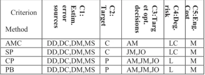
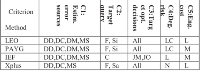
Table 1. Comparison of cardinality injection methods

Criterion Method C 1 : E st im . e r ro r so u r ce s C 2 : T a r g e t q u e r y C 3 :T a rg e t o p t. d e c is io n s C 4 :D e g . r isk C5 :E n g . c o st LEO DD,DC,DM,MS F, Si All LC L PAYG DD,DC,DM,MS F, Si All LC M IEF DD,DC,DM,MS C JM,JO L M Xplus DD,DC,MS F, Sa All N L

3.2 Plan Modification

With this different strategy, the optimizer uses catalog statistics to generate a plan. However, the execution plan is monitored at run-time. Once a sub-optimality is detected, the plan is modified: either by rescheduling, or by re-optimization. Rescheduling is to update only the execution order of the operators or to update the order of the base relations. Re-optimization is to generate a new plan for the remainder of the query using run-time collected statistics. Based on the new cost estimation, re-optimization might throw away the intermediate results and start a new plan from scratch.

3.2.1 Rescheduling

In distributed environments, the relations participating in a query plan are often stored in remote sites, and the arrival of data may be delayed. In this situation, to avoid idling, Amsaleg et al proposed a query plan scrambling algorithm [2]. The algorithm contains two phases: (1) materializing sub-trees. During this phase, each iteration of the algorithm identifies a plan fragment that is not dependent on any delayed data (the fragment is called a “runnable sub-tree”), then the fragment is executed and the result is materialized. (2) Creating new joins between relations that were not directly joined in the original query tree. When no more runnable sub-trees can be found by Phase 1, the scrambling algorithm moves into Phase 2, so that the plan execution could continue.

Query plan scrambling can improve the response time in many cases, but it only deals with the initial delay (i.e., the arrival of the first tuple is delayed). If the delay happens during the execution of the fragment, it is blocked and has to wait. To solve this problem, Bouganim et al proposed a dynamic query scheduling strategy (DQS) [12] that interleaves the scheduling phase and the execution phase. Each time, the scheduler only schedules the query fragments that can be executed immediately (i.e., all their inputs are available and there is enough memory). These fragments are executed concurrently. During execution, the data arrival rate is monitored

continuously. Once a problem is detected or the execution is finished, rescheduling is triggered. If the rescheduling cannot solve the problem, a re-optimization (see Section 3.2.2) may be triggered.

3.2.2 Re-optimization

The dynamic Re-Optimization (ReOpt) algorithm proposed by Kabra et al [46] detects the estimation errors during query execution and re-optimizes the rest of the query if necessary. At specific intermediate points in the query plan, statistics collector operators are inserted to collect various statistics. During query execution, the collected statistics are compared with the estimated ones. If there is a large difference, some heuristics are triggered to evaluate whether a re-optimization is beneficial. If so, the optimizer is recalled to modify the execution plan for the rest of the query. Instead of suspending a query in mid-execution, the currently executing operator is run to completion and re-directs the output to a temporary file on disk. Then, SQL corresponding to the rest of the query is generated by using this temporary file. The new SQL is re-submitted to the optimizer as a regular query. In ReOpt, if the difference between the collected parameter value and the estimated one exceeds a threshold, the re-optimization procedure will be considered. A later work [50] argued that this threshold is chosen arbitrarily so could be blind. [50] introduced POP algorithm which uses the “validity range” concept of the chosen plan for each input parameter. If the actual value of the parameter violates the validity range, a re-optimization is triggered; otherwise, the current plan continues execution. The violation of validity ranges is detected by a CHECK operator. Another difference between POP and ReOpt is that, when a re-optimization is triggered, ReOpt always modifies the plan for the remainder of the query in order to reuse the intermediate results, while POP allows the optimizer to discard the intermediate results and choose a completely new plan, if the cost model estimates that is to be beneficial. Han et al [37] extended the POP algorithm to a parallel environment with a shared-nothing architecture.

Continuous query optimization (CQO) [15] extends ReOpt for query optimization in massively parallel environments. On the same principle, query execution is continuously monitored, run-time statistics are collected and the parallelism degree or the partition key choice is dynamically modified.

Re-optimization is also applied for recursive queries in [28], where the estimation errors may be propagated to later iterations. The authors proposed two mechanisms. The first mechanism is called “lookahead planning”: the optimizer generates plans for k iterations, the executor executes them, provides collected statistics, and then the optimizer generates plans for the next k

iterations using these statistics, and so on. The second mechanism is called “dynamic feedback”: it detects the divergence of the cardinality estimates and decides to re-optimize the remainder of the running plan if needed. The proposal is named “lookahead with feedback” (LAWF).

Bonneau et al [11] and Hameurlain et al [36] focused on the re-optimization problem for the shared-nothing architecture and the multi-user environment. The main objective is to improve the physical resource (CPU and memory) allocation by exploiting the collected statistics at run-time. When an estimation error is detected, they re-optimize not only the mapping between the remaining tasks and the CPUs, but also the allocation of memory. Incremental memory allocation (we call it IMA in short) heuristics were proposed to avoid unexpected extra I/Os caused by lack of memory. During re-optimization, the parallelism degree may also be modified to satisfy the memory requirements.

3.2.3 Comparison

In Table 2, we compare the above methods using the five criteria. C1: The rescheduling methods were mainly designed to deal with data arrival delay and rate changing problems, while the re-optimization methods were originally used to solve the other estimation error problems. However, they are not contradictory and can co-exist to handle both kinds of problems, as Tukwila [44] does. In CQO, statistics are missing during optimization. In IMA, the unavailability of resources is also taken into account. C2: They all optimize the currently running query. C3: They focus on different decision aspects, but none of them deal with all aspects. C4: Scrambling may degrade the performance dramatically if a bad join order is chosen during Phase 2. DQS reduces this risk by estimating the increased cost before changing the join order. ReOpt reacts to every detected estimation error. When there is only one wrongly estimated parameter, it works very well. However, when there are many uncertain parameters, each re-optimization may generate just another wrong plan. POP, LAWF and IMA may face the same problem. We consider the degradation risk level as high. CQO is different, because for the moment, it only modifies parallelism degree and partition key. The decision is based on run-time collected statistics, so the degradation risk is rather low. C5: Scrambling only modifies slightly the scheduler in order to detect data arrival delays and run the two phases iteratively. DQS not only rewrites the scheduler, but also modifies slightly the optimizer to generate annotated query plans and enhances the executor to be able to interact with the scheduler. Re-optimization methods only add statistics collectors and re-optimization triggers, except POP. It suspends the query during re-optimization, and

it provides different strategies for placing the CHECK operators, in order to support pipelined execution.

Table 2. Comparison of plan modification methods

Criterion Method C 1 : E st im . e r ro r so u r ce s C 2 :T a rg e t q u e ry ty p e s C 3 :T a rg e t Op t. d e c is io n s C 4 :D e g . r isk C 5 :E n g . c o st Scrambling AD C OEO,JO H L DQS AD,AR C OEO,JO L M ReOpt DD,DC,DM C JM,JO,MA H L POP DD,DC,DM C AM,JM,JO H M CQO MS C PD,PK L L LAWF DD,DC,DM,MS C AM,JM,JO H L

IMA DD,DC,DM,UR C CA,MA,PD H L

3.3 “Robust Plan” Selection

In section 3.2, were presented the methods which react to estimation errors by modifying the plan; in this section, are examined the methods which take into account the uncertainty during optimization process. Instead of an “optimal” plan, they choose a “robust” plan.

3.3.1 Robust cardinality estimation

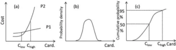
The traditional sampling-based cardinality estimation methods compute a single-point value: if the population size is N, the sample size is s, and the observed cardinality for the sample is C’, then the estimated cardinality C for the whole dataset should be C’*N/s. The estimation error could be small; however, the optimizer may still make a big mistake when choosing the plan. For example, in Figure 2 (a), we have two candidate plans P1 and P2 for query Q, where x-axis represents the value space of the uncertain cardinality and y-axis represents the cost of the plan. Suppose that the real cardinality is between Clow and Chigh. If the estimated cardinality is Clow, the

optimizer will choose P2. Otherwise, if the estimated cardinality is Chigh, the optimizer will choose P1. By

comparing these two situations, we find that the first one is more risky, because the worst case cost is high.

Figure 2. Robust cardinality estimation

Instead of estimating the cardinality by a single value C, the Robust Cardinality Estimation (RCE) method in [8] derives a probability density function of C from the sampling result, as shown in Figure 2(b). Then it transforms the probability density function into a cumulative probability function cdf(c), as shown in Figure 2(c). The user is allowed to choose a confidence threshold T which represents the level of risk (a big T corresponds to a small risk). The estimated cardinality

is computed by: C = cdf-1(T). For example, if T=95%, the model returns Chigh as the estimated cardinality, so

the more stable plan P1 will be chosen. If T=50%, the more risky plan P2 will be chosen. The authors claim that this solution is robust, because users are aware of the risk and take the responsibility for it.

3.3.2 Proactive re-optimization

Babu et al [7] proposed another way to take into account the estimation uncertainty during optimization process. In the Rio prototype, the authors estimate cardinalities using intervals, instead of single point values. If the optimizer is very certain of the estimate, then the interval should be narrow; otherwise, the interval should be wider. Using intervals allows the optimizer to generate robust plans that minimize the need for re-optimization. A robust plan is a plan whose cost is very close to optimal at all points within the interval. For example, in Figure 2(a), we assume that the estimated cardinality is Clow and the actual

cardinality is Chigh. With re-optimization methods such

as POP, the optimizer will first choose P2 which is optimal at point Clow, and then choose P1 during

re-optimization. For more complicated queries (e.g., with multiple joins and selection predicates), the situation could be even worse: re-optimization may happen repeatedly when multiple errors are detected.

We come back to the example in Figure 2(a). With Rio, the cardinality could be estimated as interval [Clow, Chigh], so P1 will be chosen directly at the

beginning, because it is robust within this interval. Thus, the re-optimization is avoided. The authors claim that their method is “proactive”, because instead of reacting to the disaster caused by a wrong plan, they tried to prevent the optimizer from choosing that plan. Unfortunately, very often, a robust plan does not exist for the estimated interval. In this case, the authors propose to choose a set of plans which are “switchable”. We will talk about this in Section 4.1. Actually, sometimes, we cannot even find a switchable plan. If this is the case, the authors propose to do like POP: choose an optimal plan using a single-point estimate and re-optimize the query if necessary. Note that, even if a robust or switchable plan is found, re-optimization may still be triggered, because the detected cardinalities may be outside of the estimated intervals.

Ergenç et al [26] extends the proactive re-optimization idea to deal with the query optimization problem in large-scale distributed environments. In such environments, the amount of data transferred between sites has a big impact on the overall performance. If the optimizer decides to place a relational operator at a wrong site due to cardinality estimation errors, huge amount of data may be transferred. To minimize the risk of wrong placement, the authors estimate the

cardinality as an interval instead of a single point value. If at any point in the interval, placing an operator on site S provides near-optimality (i.e., the performance degradation compared to the optimal placement is less than a threshold), then the site S is called a robust site. A Robust Placement (RP) for a query is to place recursively each operator in the plan tree on a robust site.

Least Expected Cost (LEC) optimization [21] also used intervals to estimate cardinalities. LEC treats statistics estimates as random variables to compute the expected cost of each plan and picks the one with lowest expected cost. It is an interesting approach for query optimization in general, but in our opinion cannot be considered as a robust optimization method, because its objective is to minimize the average running time of a compile-once-run-many query, but not to improve the worst case performance of a specific query execution.

3.3.3 Robust plan diagram reduction

A “plan diagram” is a color-coded pictorial enumeration of the plans chosen by the optimizer for a parameterized query template over the relational selectivity space [60]. The diagram is generated offline [57] by repeatedly invoking the query optimizer, each time with a different selectivity value. Then, for an instance of the query template, the optimizer first calls the selectivity estimator, and then picks the corresponding plan from the diagram. In the original paper, the authors gave examples with two-dimensional diagrams, each dimension representing the possible selectivity of one parametrized predicate in the query template. In this paper, for ease of comprehension, we illustrate the principle with a one-dimensional example. The sample query is “select * from R, S where R.A2 = S.A2 and R.A1 = $x”, where

$x is a variable. Figure 3(a) shows the diagram in the lower part, and the corresponding cost function curves above for more information. For example, if the estimated selectivity is between b and c, plan P3 will be chosen.

Using the plan diagram can avoid running the complete optimization algorithm for each instance of the parametrized query, thus the query optimization is more efficient. However, a plan diagram may contain a large number of plans in the selectivity space, making the diagram maintenance difficult. Therefore, Harish et al [38] proposed to reduce the dense diagrams to simpler ones, without degrading too much the quality of each individual plan. The principle is as follows: a plan Pa can be replaced by another plan Pb if and only if at each query point covered by Pa, the increased cost

(C(Pb) – C(Pa)) is less than a tolerance threshold

defined by the user (such as 10%). For example, P1 and P3 can be replaced by P2, as shown in Figure 3(b).

When the cardinality estimation is precise, the reduced plan diagram does not degrade the performance too much compared to the original diagram. However, when there are estimation errors, use of the reduced diagram could be at high risk. For example, with the reduced diagram in Figure 3(b), if the estimated selectivity is between b and c, P2 will be chosen. However, if the actual selectivity is much higher than c, the cost of P2 becomes very high compared to P3.

Figure 3. Example of robust plan diagram reduction

To reduce this risk, the same authors [39] proposed to make the plan replacement policy stricter: during the plan reduction, a plan Pa can be replaced by another plan Pb only if at each query point in the whole selectivity space, the increased cost (C(Pb) – C(Pa)) is less than a tolerance threshold defined by the user. Considering this condition, P3 cannot be replaced anymore, so we get the reduction result in Figure 3(c). This reduction is called “Robust Diagram Reduction” (RDR), because the risk of significant performance degradation is limited in case of estimation errors.

3.3.4 Comparison

The above methods are compared in Table 3. C1: They all assume that the running environment is stable. RCE derives the probability density function by using fresh random samples which are pre-computed manually or updated periodically whenever a sufficient number of database modifications have occurred. Thus, it does not deal with DM and MS. Rio and RP still work when catalog statistics are missing or outdated. However, their effectiveness may be affected. In fact, they compute the estimation intervals based on catalog statistics. If statistics are missing or outdated, it may happen that the intervals become too large for the optimizer to find a robust plan, or that the intervals are erroneous and re-optimization should be triggered. RDR has no constraints on estimation error sources. C2: They all deal with the currently running query, except RDR, which works for predefined parametrized queries. C3: RCE, Rio, RDR could avoid wrong decisions on base relation access methods, join methods and join ordering; RP extends Rio to improve the execution site selection. C4: RCE allows the user to choose the risk level. For Rio, if the actual cardinalities fall into the estimated intervals, and if a

robust plan exists, then the performance degradation risk is limited to a predefined threshold. However, these two conditions are difficult to satisfy. RP has the same risk level as Rio. The degradation risk of RDR is always limited, thanks to the strict replacement policy. C5: RCE only modifies the cardinality estimation module of the optimizer. Rio requires more modifications to the DBMS engine. RP works for large-scale distributed environments and is based on a mobile execution model [4]. Similar to Rio, it also requires significant modifications to the optimizer in order to support the interval-based estimation. RDR develops a stand-alone tool to prepare a set of robust plans for a predefined query template.

Table 3. Comparison of robust plan selection methods

Criterion Method C 1 : E st im . e r ro r so u r ce s C 2 : T a rg e t q u e r y ty p e s C 3 : T a r g e t o p t. d e c is io n s C 4 :D e g . r isk C5 :E n g . c o st RCE DD,DC C AM,JM,JO UC L Rio DD,DC,DM,MS C AM,JM,JO LC M RP DD,DC,DM,MS C AM,JM,JO,ES LC M RDR DD,DC,DM,MS P AM,JM,JO L L

4. MULTI-PLAN BASED APPROACH

4.1 Deferred Plan Choosing

Parametric query optimization process [10] determines for each point in the parameter space, an optimal plan. It defers choosing the plan until the start of execution. However, its objective is to avoid compiling the query for each run, but not to achieve robustness. In this section, we will study other methods, which make the choice in the middle of execution.

4.1.1 Access method competition

Whether to use indexes and which ones to use for a single-relation access depends strongly on the selectivity of the predicate. To avoid wrong optimization decisions due to the selectivity estimation uncertainty, Antoshenkov [3] proposed access method competition (AMC), i.e., to run simultaneously different base relation access processes for a small amount of time. The author argues that there is a high probability that one of them finishes during this time, and others can be canceled. Otherwise, if none of them finishes quickly, the execution engine should guess and continue only one that has the least estimated cost.

4.1.2 Plan switching

In Rio [7], if the optimizer fails to find a robust plan within the estimated interval, it tries to find a “switchable plan” (SP), which is a set S of plans such that: (1) at any point in the intervals, there is a plan p in S whose cost is close to optimal; (2) according to the detected statistics, the system can switch from one plan to another in S without losing any significant fraction of work done so far. Figure 4 gives an example of a

switchable plan. Assuming that the result size of RڇS is estimated to be small, then the first plan is executed; during execution, if the tuples produced by Rڇ S cannot fit in memory, the second plan will be switched on (i.e., changing the join algorithm from NLJ to HJ); later on, if the result size of RڇS is detected to be much bigger than the relation T, the third plan will be switched on. The switching process is smooth thanks to a “switch” operator integrated in the plan tree.

Figure 4. Example of a switchable plan

The “switch” operator can be seen as a variant of the “choose-plan” operator (CP) proposed earlier by Graefe et al. in [29]. “Choose-plan” operators are run-time primitives that permit optimization decisions to be prepared at compile-time and evaluated at run-time. It was initially designed to deal with the situation where parameters in the query template are unknown; however, other estimation errors like non-uniform distribution could also be addressed by adding a “choose-plan” operator at an appropriate position in the decision tree.

A different way of switching plans based on “Plan Bouquets” (PB) has been proposed recently [25]. First, through repeated invocations of the optimizer, a “parametric optimal set of plans” (POSP) that covers the entire selectivity space of the predicates is identified. Second, a “POSP infimum curve” (PIC) which is the trajectory of the minimum cost from the POSP plans is constructed. Then, the PIC is discretized by some predefined isocost (IC) steps, IC1, IC2, … , which are progressive cost thresholds, for example, each IC value doubles the preceding one. The intersection of each IC with the PIC corresponds to a selectivity value and the best POSP plan for this selectivity. The set of plans associated with these ICs is called a “Plan Bouquet”. At run-time, the plan associated with the cheapest IC step is executed first. If the partial execution overheads exceed the IC value, it means that the actual selectivity is beyond the range where the current plan is optimal, so a switch to the plan associated with the next IC value is triggered. Otherwise, if the current plan completes execution before reaching the IC value, it means that the actual selectivity is inside the range covered by this plan. Since the cost of executing a sequence of plans before discovering the actual selectivity and then switching to the optimal plan is bounded by the IC values, Plan Bouquet method guarantees worst-case performance.

4.1.3 Comparison

In Table 4, we compare the above methods. C1: They deal with all kinds of estimation errors in a stable environment. C2: AMC and SP work for the currently running query, while CP and PB were initially designed for predefined parametrized queries. C3: AMC focuses on base relation access method selection; SP deals with join methods and join order; CP and PB cover all those three decisions. C4: AMC has low degradation risk, at the condition that one of the concurrent processes finishes quickly; SP also has low degradation risk, at the condition that the actual cardinalities are inside the estimated intervals. CP and PB have low degradation risk. C5: All methods require major modifications to the optimizer and the executor.

Table 4. Comp. of deferred plan choosing methods

Criterion Method C 1 : E st im . e r ro r so u r ce s C 2 : T a r g e t q u e r y C 3 :T a rg e t o p t. d e c is io n s C 4 :D e g . r isk C5 :E n g . C o st AMC DD,DC,DM,MS C AM LC M SP DD,DC,DM,MS C JM,JO LC M CP DD,DC,DM,MS P AM,JM,JO L M PB DD,DC,DM,MS P AM,JM,JO L M

4.2 Tuple Routing through Eddies

With the methods described in Section 4.1, although the optimizer proposes multiple execution plans, only one of them “survives”. Thus, all tuples flow through the same plan tree (route). Differently, Avnur et al [5] allow different tuples to flow through different routes using a special operator “eddy”. The eddy mechanism was extended for different environments [59, 64, 70].

4.2.1 The eddy

A tree-like plan fixes the execution order of the operators in advance, i.e., tuples always flow from leaves to the root. This order can be changed at run-time by using rescheduling or re-optimization, but it is too costly to change it frequently. Avnur et al. [5] proposed a more flexible mechanism which can continuously reorder the operators. They use a star-like query plan, where the relational operators surround a coordinating operator called an eddy. Tuples from base relations and intermediate results are sent to the eddy which routes each tuple to an operator according to the routing policy. The eddy sends a tuple to the output only if it has been handled by all the operators. We illustrate the effectiveness of eddies using the query “select * from R, S, T where R.B=S.B and S.C=T.C”. Suppose that tuples arrive from the three relations with different delay and rate. In the plan, if there are two join operators Op1 (Rڇ S) and Op2 (SڇT), tuples from R can be only routed to Op1, and tuples from T can be only routed to Op2, while tuples from S can be routed either to Op1 or to Op2. The

eddy makes the routing decision for tuples from S dynamically according to a predefined policy, which tries to minimize the execution cost. A specific join algorithm called Symmetric Hash Join (SHJ) [68, 41] is recommended: two hash tables are maintained, one for each input relation; the arriving tuple is built immediately into the corresponding hash table and probed against the existing tuples in the other hash table, so the intermediate result can be produced immediately and returned to the eddy. This is actually the “secret” of eddies to enable the reorder-ability: (1) the operator state is continuously maintained, regardless of the execution order; and (2) the “faster” relation is never blocked by the “slower” relation. We can find that, an eddy is equivalent to a set of tree-like query plans, each one handling a subset of tuples. The tuple routing policy is used to make the mappings. Advanced routing policies [9] were proposed later on. Note that, since the eddy implementations rely on the symmetric hash join, they are more adequate to streaming scenarios where existing relations fit in memory.

4.2.2 Extensions of the eddy

The adaptability of the eddy is limited to operator re-ordering, whereas access methods and join algorithms are pre-chosen and fixed during the execution. A more flexible version [59] also allows continuously changing the choice of access methods and join algorithms, etc. To do this, Raman et al [59] made the following main modifications to the eddy architecture: (1) each join operator is replaced by two State Modules (SteMs) which encapsulate data structures (such as hash tables or indexes) used in join algorithms; (2) one or several Access Modules (AMs) are added to each base relation, each AM encapsulating one access method to the data source; and (3) new routing policies are used by the eddy module. At the beginning, different AMsare run concurrently (thus redundantly). In fact, they are in competition: when the eddy finds that one is much more efficient than the others, it will stop the slower ones. Tian and DeWitt [64] extended the eddy and SteMs architecture to a distributed version. Instead of using a centralized eddy module which could become a bottleneck, the authors proposed to integrate the routing function into each operator. Zhou et al [70] designed another distributed query processing architecture called SwAP, building on eddies and SteMs. The authors proposed to use one eddy module for each execution site, which routes tuples between the local operators and remote eddies.

4.2.3 Comparison

We compare the tuple routing methods in Table5. C1: They deal with all kinds of estimation errors. C2: They optimize the currently running query. C3: Eddy only

optimizes the join order and operator execution order; the extensions of eddy also optimize base relation access methods and join methods. C4: Although there is no theoretical guarantee, Deshpande [23] has shown experimentally that the performance degradation of eddies is low. Other methods have the same risk level, under the condition that one of the competing access methods wins quickly. C5: In these methods, most of the optimization decisions are made by the eddy module, so the classical optimizer is reduced to a pre-optimizer, and the execution engine becomes more complicated. Thus, the engineering cost is high.

Table 5. Comparison of tuple routing methods

Criterion Method C 1 : E st im. e r ro r so u r c es C 2 : T a rg e t q u e r y t y p e s C 3 : T a r g e t o p t. d e c is io n s C 4 :D e g . r isk C 5 :E n g . C o st

Eddy All C JO,OEO L H

SteM All C AM,JM,JO,OEO LC H Tian All C AM,JM,JO,OEO LC H SwAP All C AM,JM,JO,OEO LC H

4.3 Optimizer Controlled Data

Partitioning

In TRE based methods, the mapping between tuples and multiple plans is decided by the eddy module, according to local indicators, such as input rate and output rate of an operator. In OCDP based methods, the mapping is decided by the optimizer, according to global statistics. TRE tends to avoid worst-case performance, while OCDP also aims at exploring best-case opportunities. We will present some representative methods in this section.

4.3.1 Run-time partitioning

Ives et al [45] proposed an adaptive data partitioning (ADP) method. During query execution, the data are dynamically partitioned into sub-datasets, each following a specific plan. Three partitioning strategies are illustrated: (1) sequential partitioning. The query execution is divided into multiple phases. All tuples arriving during Phase PhN follow a plan PlN. PlN is

chosen using the statistics collected during the previous N-1 phases. To guarantee the correctness of the result, a “stitch-up” phase is added at the end. For example, two relations S and T are joined through two phases. During Ph0, S0 and T0 are joined; during Ph1,

S1 and T1 are joined. According to the following

equation: SڇT = (S0ڇT0) U (S1ڇT1) U (S0ڇT1) U

(S1ڇT0), the “stitch-up” phase has to compute (S0ڇT1)

and (S1ڇT0). (2) Dynamic splitting. Multiple plans are

run concurrently, and the arriving tuple is sent to one plan by a “split” operator according to some criteria. For example, to join two relations which are quasi-sorted, tuples respecting the expected order will be sent

to the plan with merge-join, and others will be sent to the plan with hash join. (3) Partitioning used for plan competition. Multiple plans are run concurrently, each processing a small subset of data. If one is much faster than the others, it will process all the remaining data. Note that, for the last two strategies, a “stitch-up” phase is also needed.

4.3.2 Compile-time partitioning

Different from ADP, Selectivity-Based Partitioning (SBP) [58] and Query Mesh (QM) model [54, 55] decide the data partitions and corresponding plans at query compile time. The author of SBP noticed that there often exist join correlations among relation fragments, for example, given two relations R and S, where S = S1׫S2, it may happen that the join RڇS1 is

selective while RڇS2 is much less selective. Based on

this observation, for a chain query with equality predicates, the author proposed to horizontally partition one relation in the chain, and rewrite the original query as the union of a set of sub-queries. For different sub-queries, the optimizer can choose several join orders, such that the overall performance is better than using a single plan without partitioning. The search space of this optimization problem is large: the optimizer has to decide which relation to partition, choose the number of partitions and compute the optimal join order corresponding to each partition. The author proposed a heuristic algorithm for computing an effective solution without exploring the complete search space. With the QM model, for a given query, a decision tree-based classifier is learned from a training dataset. Each decision node is a predicate (such as A>x) which distributes the arriving tuples into different classes. For each tuple class, a best plan is chosen. The choice of execution plans and the classifier are mutually dependent, so they should be considered as a whole, meaning that the execution cost of each plan for each possible data subset should be estimated and compared. The search space is too big to use an enumerative search strategy, so the authors chose randomized search strategies. Similar to QM, correlation-aware multi-route stream query optimizer (CMR) [16] also partitions the data and computes an optimal plan for each partition. The difference is that it explores explicitly data correlations, which not only makes the partitioning more effective but also reduces the optimization complexity. Horizontal Partitioning with Eddies HPE [65] is another work using different plans for different data partitions. The originality is: first, the authors introduced the notion of conditional join plans (CJP), a new representation of search space which captures both the partitioning and the join orders for each partition combination; second, they use the eddy mechanism as the execution model, in order to share intermediate results between different plans.

4.3.3 Comparison

We compare the above methods in Table 6. C1: They are all resistant to (or even take advantage of) non-uniform data distribution and data correlations. HPE uses eddies, so it is also resistant to data arrival delay and rate changing, etc. C2: They all optimize the current query. C3: SBP focuses only on join order. Others focus also on access methods and join methods. Again, with eddies, HPE can also optimize the operator execution order. C4: The degradation risk is low, because characteristics of each sub-dataset are well-known by the optimizer. C5: The engineering cost is high, because both the optimizer and the plan executor need to be rewritten.

Table 6. Comparison of data partitioning methods

Criterion Method C 1 : E st im . e r ro r so u r ce s C 2 :T a rg e t q u e r y t y p e s C 3 : T a r g e t o p t. d e c is io n s C 4 :D e g . r isk C 5 :E n g . c o st SBP DD,DC C JO L H ADP DD,DC C AM,JM,JO L H QM DD,DC C AM,JM,JO L H CMR DD,DC C AM,JM,JO L H HPE All C AM,JM,JO,OEO L H

5. GLOBAL COMPARISON

In this section, we make a global comparison of the two approaches and their adopted strategies. With single-plan based approach, methods are easier to implement, but none of them can handle all types of estimation error sources; different methods could be combined to enlarge the application scope, but when there are too many uncertain factors, the degradation risk becomes high. With multi-plan based approach, the degradation risk is limited, but the engineering cost is higher. Eddy-based methods can handle all kinds of estimation error sources, however, most of them require that the hash tables fit in memory. In addition, how eddies can be used in a highly parallel environment has not been well studied.

In Table 7, we list briefly the advantages and limitations of the strategies used by each approach.

6. CONCLUSION

Robust query optimization methods take into account the uncertainty of estimated parameter values, in order to avoid or recover from bad decisions caused by estimation errors. In this paper, the representative methods were classified into two main approaches: single-plan based approach and multi-plan based approach. For each approach, we highlight the principle strategies. We analyzed and compared the methods using five well-selected criteria: estimation error sources, target query types, target optimization decisions, performance degradation risk and

engineering cost. Finally, a global comparison of the approaches and the strategies is given.

Table 7. Global comparison

Approach Strat egy Advantage Limitation Single- Plan Based CI Good for repeatedly-running queries

For current query, only JM, JO are optimized

PM Could be extended to improve all kinds of opt. decisions

May have high degradation risk RPS Degradation risk is

low if a robust plan exists

Difficult to handle too many uncertain factors Multi- Plan Based DPC Easier to implement than TR and DP

AMC may consume too many resources TRE Deal with all kinds

of estimation error sources

Memory consuming; Parallelization problem not addressed OCD P Take advantage of inherent data characteristics Optimization time may be long

The main conclusions to be drawn are: (1) different strategies of the single-plan based approach can be combined to enlarge the application scope, as the AutoAdmin project [14] does, (2) single-plan based approach is easier to be integrated into the main commercial DBMSs, but it only works well when there are few uncertain parameters, and (3) hence when there are too many uncertain parameters, the multi-plan based approach is a safer choice.

7. REFERENCES

[1] Aboulnaga, A. and Chaudhuri, S. 1999. Self-tuning Histograms: Building Histograms without Looking at Data. In

SIGMOD. New York, USA, 181-192.

[2] Amsaleg, L., al.1996. Scrambling Query Plans to Cope with Unexpected Delays. In PDIS. Miami, USA, 208-219. [3] Antonshenkov, G. 1993. Dynamic Query Optimization in

Rdb/VMS. In ICDE. Vienna, Austria, 538-547.

[4] Arcangeli, J.P., et al. 2004. Mobile Agent Based Self-Adaptive Join for Wide-Area Distributed Query Processing. Journal of

Database Management, 15(4): 25-44.

[5] Avnur, R. and Hellerstein, J.M. 2000. Eddies: Continuously Adaptive Query Processing. SIGMOD. Dallas, USA, 261-272. [6] Babu, S. and Bizarro, P. 2005. Adaptive Query Processing in

the Looking Glass. In CIDR. Asilomar, USA, 238-249. [7] Babu, S., et al. 2005. Proactive Re-Optimization. In SIGMOD.

Baltimore, USA, 107-118.

[8] Babcock, B. and Chaudhuri, S. 2005. Towards a Robust Query Optimizer: A Principled and Practical Approach. In SIGMOD. Baltimore, USA, 119-130.

[9] Bizarro, P., et al. 2005. Content-Based Routing: Different Plans for Different Data. In VLDB. Trondheim, Norway, 757-768.

[10] Bizarro, P., et al. 2009. Progressive Parametric Query Optimization. KDE, 21(4): 582 – 594.

[11] Bonneau, S. and Hameurlain, A. 1999. Hybrid Simultaneous Scheduling and Mapping in SQL Multi-Query Parallelization. In DEXA. Florence, Italy, 88-98.

[12] Bouganim, L., et al. 2000. Dynamic Query Scheduling in Data Integration Systems. In ICDE. San Diego, USA, 425-434. [13] Bruno, N., et al. 2001. STHoles: a multidimensional