O
pen
A
rchive
T
OULOUSE
A
rchive
O
uverte (
OATAO
)
OATAO is an open access repository that collects the work of Toulouse researchers and
makes it freely available over the web where possible.
This is an author-deposited version published in :
http://oatao.univ-toulouse.fr/
Eprints ID : 15324
The contribution was presented at EMBC 2015 :
http://embc.embs.org/2015/
To cite this version : Chen, Zhouye and Basarab, Adrian and Kouamé, Denis A
simulation study on the choice of regularization parameter in l2-norm ultrasound
image restoration. (2015) In: 37th Annual International Conference of the IEEE
Engineering in Medicine and Biology Society (EMBC 2015), 25 August 2015 - 29
August 2015 (Milano, Italy).
Any correspondence concerning this service should be sent to the repository
administrator:
[email protected]
A simulation study on the choice of regularization parameter in
ℓ
2-norm ultrasound image restoration*
Zhouye Chen, Adrian Basarab, Denis Kouam´e
Abstract— Ultrasound image deconvolution has been widely investigated in the literature. Among the existing approaches, the most common are based on ℓ2-norm regularization (or Tikhonov optimization) or the well-known Wiener filtering. However, the success of the Wiener filter in practical situations largely depends on the choice of the regularization hyperpa-rameter. An appropriate choice is necessary to guarantee the balance between data fidelity and smoothness of the decon-volution result. In this paper, we revisit different approaches for automatically choosing this regularization parameter and compare them in the context of ultrasound image deconvolution via Wiener filtering. Two synthetic ultrasound images are used in order to compare the performances of the addressed methods.
I. INTRODUCTION
Ultrasound (US) medical imaging has the advantages of being noninvasive, harmless, cost-effective and portable over many other imaging modalities such as X-ray computed tomography or Magnetic Resonance Imaging [1]. However, the limited bandwidth of the imaging transducer, the char-acteristics of the ultrasound propagation such as diffraction and the imaging system tend to degrade the quality of the US images. To deal with this problem, significant efforts have been made in the last few decades.
Under some weak assumptions (first order Born ap-proximation and weak scattering), the recorded US radio-frequency image can be modeled as the result of a 2D convolution between the tissue reflectivity function and the point-spread function (PSF) [2]. As a consequence, deconvo-lution methods have been intensively considered to enhance the spatial resolution of US images. Among the existing approaches, Wiener filtering (and variants) was one of the most explored tracks in US imaging [3], [4]. However, it is well-known that the results of the Wiener filter or its variants largely depends on the choice of the regularization parameter (RP) that provides a compromise between data fidelity and smoothness of the deconvolution result. In US imaging, the choice of the RP is either done manually (empirically or by trial-and-error) [3], or is simply related to the signal-to-noise ratio (the RP is considered the inverse of the SNR) which is further estimated from the data [4]. In the general literature related to Wiener filter deconvolution, several approaches have been proposed to find an optimal value of RP in an automatic manner. In this paper, we propose to evaluate and compare their performances in the framework of ultrasound imaging. To do so, two simulated US images are used.
The remainder of the paper is organized as follows. The considered model and the Wiener filtering approach are presented in Section II. Section III reviews the existing approaches of optimal RP choice. The simulation setup, the deconvolution results and the comparison in US imaging are provided in Section IV.
II. PROBLEM FORMULATION
Under the assumption of weak scattering and using the first order Born approximation, the interaction between the tissues and the propagating ultrasound waves is classically modeled by the following 2D convolution model [2]:
y= Hx + n (1) where y ∈ RM N ×1 is the vertical concatenation of M
acquired radio-frequency (RF) signals of length N (also known as ”lexicographical notation” of the RF image), x∈ RM N ×1 is the tissue reflectivity function using the same lexicographical notation, H∈ RM N ×M Nis a block circulant
with circulant block (BCCB) matrix related to the 2D PSF of the system and n∈ RM N ×1 is a zero-mean additive white
Gaussian noise with variance σ2. The purpose of non-blind
deconvolution methods is to recover the tissue reflectivity function x from the recorded US RF image y considering the PSF known (or provided a previous estimate of the PSF). A common way to solve the non-blind deconvolution problem is the well-known Wiener/Tikhonov approach, that provides the following analytical estimation of x:
ˆ
x= (HtH+ λQtQ)−1Hty= F (λ)y (2) wherexˆis the estimate of x, and Q∈ RM N ×M Nis a BCCB matrix representing the regularization operator, classically considered the identity matrix or the 2D Laplacian opera-tor. λ is a hyperparameter providing compromise between data fidelity and smoothness of the estimate (addressed as regularization parameter (RP) hereafter). The value of λ that guarantees an optimal compromise between data fidelity and smoothness depends on the variance of the noise σ2and on
the properties of H, Q and y [5].
III. METHODS FOR REGULARIZATION PARAMETER OPTIMAL CHOICE
In the general Wiener filtering literature, several ap-proaches have been proposed to automatically fix the value of the RP λ [6]. We review hereafter the main approaches, that we further evaluate in the context of US images. Following [6], we classify them into two categories. The first includes methods that need the knowledge of the variance of the noise
(or an estimate of it) to estimate the RP, while the second one does not have this constraint.
A. Methods with knowledge of the variance of the noise 1) Constrained least squares (CLS): The principle of this method, originally proposed in [7], is based on the residual between the data y and Hxˆ for a given λ, expressed as:
φ(λ) =k y − H ˆxk22=k y − HF (λ)y k22 (3) The optimal λ in the sense of CLS is obtained in the case where the residual in (3) is equal to the variance of the noise, or more precisely to M N σ2. From this it results an
equation with the unknown λ, which was shown in [7] to have an unique solution. This optimal value of λ, that we will denote by λCLS in this paper, is obtained by solving
the above equation using a numerical iterative procedure. 2) Degree of freedom (EDF): Similar to CLS approach, the equivalent degree of freedom method [8] estimated the RP λ from an equation relating the residual and the variance of the noise. Based on the linear relation between y andx,ˆ the residual in (3) is further expressed as:
φ(λ) = σ2trace[I
M N− HF (λ)] (4)
where IM N ∈ RM N ×M N is the identity matrix.
The optimal RP given by EDF approach will be denoted hereafter by λEDF.
3) Mean square error (MSE): The main idea behind this method is to find the value of λ that minimizes the mean square error between x and its estimate, denoted by ǫ(λ): E(k ǫ(λ) k2
2) = E[k ˆx−x k22] =k x k22+E[k ˆxk22]−2E[ˆx tx]
(5) In order to eliminate the cross-term 2E[ˆxtx], which is impossible to compute in practice because of the non-knowledge of x, it is replaced in [6] by a term depeding on the data y and on the noise variance σ2, based on a circulant
assumption in DFT domain. In this case, it is shown in [6] that minimizing (5) with espect to λ is equivalent to soving the following equation:
k Q−1(I M N−HF (λ)) 3 2 yk22= σ2trace[Q−2(IM N−HF (λ))2] (6) We denote by λM SE the value of λ verifying (6) and
obtained in practice with numerical optimization techniques. 4) Predicitve mean square error (PMSE): Similar to the previous approach, this method is also based on the minimization of the MSE between x and its estimate. More precisely, a weighted ℓ2 error norm E[k Hǫ(λ) k2
2], also
called the predictive mean square error, is minimized [5], [9], [10]. Following the same assumptions as the previous approach, this minimization turns out in solving the equation hereafter:
E[k Hǫ(λ) k2
2] =k (IM N−HF (λ))y k22+2σ2trace[HF (λ)]
(7) The solution of (7), obtained by numerical optimization, is called λP M SE in what follows.
5) Generalized Stein’s unbiased risk estimate (GSURE): The main idea behind this method is to find the RP that minimizes the following error measure between x and its estimate [11], [12]:
e(λ) =k P (x − ˆx) k2 (8)
where P= Ht(HHt)†H is the projection operator and(·)†
represents the pseudo-inverse.
Keeping in mind that the Wiener filter, given a value of λ, provides an analytical relation betweenxˆ and y, we denote by f a function from RM N to RM N with xˆ = f (y). As shown in [10], [11] and [12], an unbiased estimator for the projected MSE in (8), depending on the variance of the noise and separating the true x from its estimation f(y), is given by: e(λ) =k P x k2+ k P f (y) k2 2−2ft(y)Ht(HHt) † y +2σ2trace(P (HtH+ λQtQ)−1) (9)
Minimizing (9) with respect to λ provides the optimal value of the RP, in the sense of GSURE approach, denoted by λGSU RE.
B. Methods without knowledge of the variance of the noise The methods presented in the previous section are all based on the knowledge of the variance of the noise. De-pending on the application, this may be an issue and a bad estimation of σ2 may cause severe errors in the optimal
choice of the RP.
In the following, we briefly describe two existing ap-proaches that do not use σ2to provide an automatical choice
of λ.
1) Generalized cross-validation (GCV): Generalized cross-validation (GCV) is one of the most popular methods of choosing optimal RP and does not require the knowledge of the noise variance σ2. Introduced in [5], its main idea is based on the ”leave-one-out” principle. In the case of linear algorithms, the GCV method leads to a simple function to minimize depending on λ: GCV(λ) = k (IM N− HF (λ))y k 2 2 [trace(IM N− HF (λ))]2 (10) The value obtained by numerical minimization of (10) is denoted by λGCV in this paper.
2) Marginal likelihood (ML): This approach is based on the minimizing of the marginal likelihood (ML) function given hereafter [6]: M L(λ) = y t(I M N− HF (λ))y (det[IM N− HF (λ)])1/M N (11) Hereafter, we denote the λ minimizing (11) by λM L.
IV. RESULTS AND DISCUSSION A. Experimental Setting
To evaluate the performance of these different methods, we used two synthetic ultrasound images. The two images were simulated by 2D convolution between realistic PSFs and the tissue reflectivity functions shown as the first images in Fig.
TABLE I: Deconvolution Results of Synthetic Ultrasound Images
SNR 10dB 20dB 30dB
Image Cyst Phantom Cardiac Image Cyst Phantom Cardiac Image Cyst Phantom Cardiac Image Lambda SSIM Lambda SSIM Lambda SSIM Lambda SSIM Lambda SSIM Lambda SSIM 1/SNR 1,00E-01 82,05 1,00E-01 63,50 1,00E-02 86,88 1,00E-02 67,29 1,00E-03 91,61 1,00E-03 76,15 CLS 2,12E-01 82,95 8,32E-01 65,32 1,60E-02 86,53 4,13E-02 67,93 1,81E-03 91,76 2,66E-03 75,24 EDF 2,73E-02 76,67 3,48E-02 61,05 2,12E-03 83,74 1,91E-03 60,24 3,18E-04 89,49 2,22E-04 67,49 MSE 2,37E-02 75,74 2,49E-02 40,46 2,25E-03 84,04 1,79E-03 59,69 4,09E-04 90,55 2,89E-04 70,56 PMSE 3,41E-02 77,98 5,84E-02 63,73 2,02E-03 83,46 2,12E-03 61,02 2,06E-04 86,59 1,79E-04 64,27 GSURE 2,37E-02 75,74 2,49E-02 40,46 2,25E-03 84,04 1,79E-03 59,69 4,09E-04 90,55 2,89E-04 70,56 GCV 3,46E-02 78,06 6,05E-02 63,80 2,02E-03 83,46 2,13E-03 61,08 2,06E-04 86,59 1,79E-04 64,27 ML 4,57E-02 79,46 2,79E-01 63,59 3,90E-03 86,04 1,51E-02 67,78 2,80E-04 88,65 7,00E-04 70,24
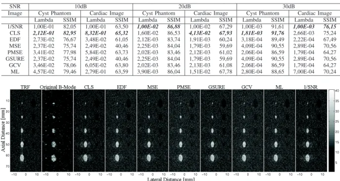
Fig. 1: SNR=30dB. From left to right, the images are Cyst phantom tissue reflectivity function, Cyst phantom B-mode US image and its deconvolution results (B-mode visualisation) for Q= I.
1 and Fig. 2. Independent and identically distributed (IID) zero- mean Gaussian noise was added to the data, yielding different SNRs. This leads to the original B-mode images, as shown in Fig. 1 and Fig. 2.
1) Cyst phantom image: For the first simulated image, the PSF was generated with Field II [13] and corresponds to a 3.5 MHz linear probe, sampled in the axial direction at 20 MHz. The tissue refelctivity function was obtained by generating scatterers at uniform random positions with random amplitudes following gaussian distribution with zero mean and variance depending on their spatial position. The medium consists in five hyperechoic circular cysts, five hypoechoic circular cysts and five point reflectors.
2) Simulated cardiac image: The PSF was also generated with Field II [13] and corresponds to a sectorial probe with the central frequency equal to 4 MHz and a axial sampling frequency of 40 MHz. The scatterer positions were uniformly random distributed. In order to obtain an ultra-realistc simulation, the amplitudes of the scatterers were related to the amplitude of an in vivo cardiac image, as suggested in [14].
B. Deconvolution Results
For both US simulations, the deconvolution results were obtained with the Wiener filtering approach, considering the true PSF known. The RP was chosen with one of the approaches in Section III or using the classical choice of λ equal to the inverse of the SNR. For the methods that need the knowledge of the SNR, the true value was employed. Two classical cases were considered using two different
regularization operators Q: the identity matrix and the 2D Laplacian operator.
TableI shows the deconvolution results for each approch of RP optimal choice. The deconvolved images are compared to the true reflectivity function using the structural similarity measure (SSIM) [15]. For each simulation and for a given SNR, we highlight in bold fonts the best result. Note that the figures we give in Table I are obtained with a regularization operator equal to the identity matrix. The results follow the same trend for a Laplacian operator.
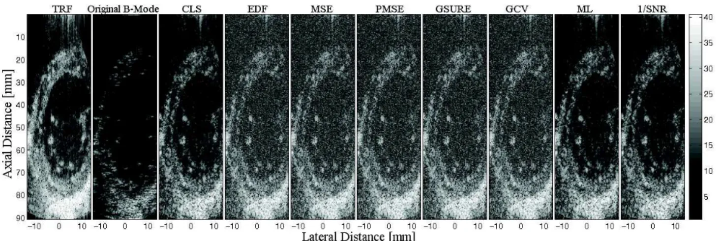
The different results may be appreciated from a quali-tative viewpoint in Fig. 1 and 2, highlighting the original refelctivity function, the data and the deconvolved images. All the processing was done in the RF domain. However, for visualisation reasons, we plot the corresponding B-mode images, obtained after log-compression of the corresponding enveloppe images.
C. Discussion
We may first remark that the different strategies of RP optimal choice provide very different values of λ and thus influence the quality of the deconvolution results. We should note that this conclusion is less true for higher SNRs (larger than 40 dB).
Second, as predicted in [5], the results provided by PMSE and GCV approaches are very similar. Similarly, the values of λM SE and λGSU RE are also very close. This is due to
the fact that both MSE and GSURE methods are based on the minimization of the MSE. Despite the different ways of minimizing the MSE, they still provide similar results.
Fig. 2: SNR=30dB. From left to right, the images are Cardiac tissue reflectivity function, Cardiac B-mode US image and its deconvolution results (B-mode visualisation) for Q= Q2DL.
Third, we may remark that the approaches that are not based on the knowledge of the SNR (GCV and ML) are still providing interesting results in US image deconvolution compared to the other approaches. The quantitative and qualitative results that we obtained point out that the ML approach is more adapted to US imaging than GCV. For all the cases, ML is among the best three methods (or very close to the best three), with CLF and the inverse of the SNR, both of which require the knowledge of the variance of the noise.
V. CONCLUSIONS
In this paper, we have compared eight methods of choos-ing optimal RP in the context of US deconvolution via Wiener filtering. The comparison was performed on two synthetic US images. An interesting conclusion is that the approaches not using the knowledge of the variance of the noise are competitive against the others and are thus very attractive in practical situations. In a future work, these results should be confirmed on experimental data, combined with approaches of PSF and noise variance estimation.
REFERENCES
[1] T. L. Szabo, Diagnostic ultrasound imaging: inside out. Academic Press, 2004.
[2] J. A. Jensen, J. Mathorne, T. Gravesen, and B. Stage, “Deconvolution of in vivo ultrasound b-mode images,” Ultrasonic Imaging, vol. 15, no. 2, pp. 122–133, 1993.
[3] O. Michailovich and A. Tannenbaum, “Blind deconvolution of medical ultrasound images: A parametric inverse filtering approach,” IEEE
transactions on image processing: a publication of the IEEE Signal Processing Society, vol. 16, no. 12, p. 3005, 2007.
[4] R. Jirik and T. Taxt, “Two-dimensional blind bayesian deconvolution of medical ultrasound images,” Ultrasonics, Ferroelectrics and
Fre-quency Control, IEEE Transactions on, vol. 55, no. 10, pp. 2140–2153, 2008.
[5] G. H. Golub, M. Heath, and G. Wahba, “Generalized cross-validation as a method for choosing a good ridge parameter,” Technometrics, vol. 21, no. 2, pp. 215–223, 1979.
[6] N. P. Galatsanos and A. K. Katsaggelos, “Methods for choosing the regularization parameter and estimating the noise variance in image restoration and their relation,” Image Processing, IEEE Transactions
on, vol. 1, no. 3, pp. 322–336, 1992.
[7] B. Hunt, “The application of constrained least squares estimation to image restoration by digital computer,” Computers, IEEE Transactions
on, vol. 100, no. 9, pp. 805–812, 1973.
[8] G. Wahba, “Bayesian” confidence intervals” for the cross-validated smoothing spline,” Journal of the Royal Statistical Society. Series B
(Methodological), pp. 133–150, 1983.
[9] P. Hall and D. Titterington, “Common structure of techniques for choosing smoothing parameters in regression problems,” Journal of
the Royal Statistical Society. Series B (Methodological), pp. 184–198, 1987.
[10] S. Ramani, Z. Liu, J. Rosen, J.-F. Nielsen, and J. A. Fessler, “Regu-larization parameter selection for nonlinear iterative image restoration and mri reconstruction using gcv and sure-based methods,” Image
Processing, IEEE Transactions on, vol. 21, no. 8, pp. 3659–3672, 2012.
[11] Y. C. Eldar, “Generalized sure for exponential families: Applications to regularization,” Signal Processing, IEEE Transactions on, vol. 57, no. 2, pp. 471–481, 2009.
[12] R. Giryes, M. Elad, and Y. C. Eldar, “The projected gsure for automatic parameter tuning in iterative shrinkage methods,” Applied
and Computational Harmonic Analysis, vol. 30, no. 3, pp. 407–422, 2011.
[13] J. A. Jensen, “A model for the propagation and scattering of ultrasound in tissue,” Acoustical Society of America. Journal, vol. 89, no. 1, pp. 182–190, 1991.
[14] M. Alessandrini, H. Liebgott, D. Friboulet, and O. Bernard, “Simu-lation of realistic echocardiographic sequences for ground-truth vali-dation of motion estimation,” in Image Processing (ICIP), 2012 19th
IEEE International Conference on. IEEE, 2012, pp. 2329–2332. [15] Z. Wang, A. C. Bovik, H. R. Sheikh, and E. P. Simoncelli, “Image
quality assessment: from error visibility to structural similarity,” Image