Localized traveling pulses in natural doubly diffusive convection

O

pen

A

rchive

T

OULOUSE

A

rchive

O

uverte (

OATAO

)

This is an author-deposited version published in : http://oatao.univ-toulouse.fr/

Eprints ID : 18604

To link to this article : DOI:10.1103/PhysRevFluids.2.093501 URL : http://dx.doi.org/10.1103/PhysRevFluids.2.093501

To cite this version : Lo Jacono, David and Bergeon, Alain and Knobloch, Edgar Localized traveling pulses in natural doubly

diffusive convection. (2017) Physical Review Fluid, vol. 2 (n° 9).

pp.093501/1-093501/19. ISSN 2469-990X

Any correspondence concerning this service should be sent to the repository administrator: staff-oatao@listes-diff.inp-toulouse.fr

Localized

traveling pulses in natural doubly diffusive convection

Institut de Mécanique des Fluides de Toulouse (IMFT), Université de Toulouse, CNRS, INPT, UPS, F-31400 Toulouse, France

E. Knobloch

Department of Physics, University of California, Berkeley, California 94720, USA

Two-dimensional natural doubly diffusive convection in a vertical slot driven by an imposed temperature difference in the horizontal is studied using numerical continuation and direct numerical simulation. Two cases are considered and compared. In the first a concentration difference that balances thermal buoyancy is imposed in the horizontal and stationary localized structures are found to be organized in a standard snakes-and-ladders bifurcation diagram. Disconnected branches of traveling pulses TPn consisting of n, n = 1,2, . . . , corotating cells are identified and shown to accumulate on a tertiary branch of traveling waves. With Robin or mixed concentration boundary conditions on one wall all localized states travel and the hitherto stationary localized states may connect up with the traveling pulses. The stability of the TPnstates is determined and unstable TPnshown to evolve into spatio-temporal chaos. The calculations are done with no-slip boundary conditions in the horizontal and periodic boundary conditions in the vertical.

DOI:10.1103/PhysRevFluids.2.093501

I. INTRODUCTION

Natural doubly diffusive convection is of considerable importance in a variety of applications, ranging from oceanography [1] to crystal growth [2]. This type of convection arises in systems driven by an imposed horizontal temperature difference or imposed horizontal heat flux when this is opposed by a compensating concentration difference or concentration flux. With fixed temperature and concentration boundary conditions this system has been studied in both two [3–5] and three dimensions [6]. For typical parameter values the onset of convection leads to stationary but subcritical states [4,5] that rapidly evolve into a state of corotating rolls, whose sense of rotation is determined by the Lewis number of the fluid. Early work has focused on the two-dimensional problem, and in particular on the onset of convection and small amplitude behavior near onset [3]. This work has demonstrated that unless the horizontal gradients are balanced exactly convection will take the form of a large cell with upflow along one sidewall and downflow along the other, provided that the system is not too extended in the horizontal. In particular, no conduction state is present, and normal convection develops as a secondary instability of this base flow. In three dimensions the spatial organization of the resulting flow depends crucially on the aspect ratio of the cavity [6,7]. Complex time dependence can result when the primary branch of steady convection fails to restabilize owing to the presence of instability with respect to convection with a different orientation, a situation that leads to strongly nonlinear oscillations near the onset of primary instability [6].

Past work has demonstrated that this system can also exhibit spatially localized convection, at least in the balanced case already mentioned. The calculations in Refs. [5,8] show that in an infinite vertical slot the subcritical primary bifurcation to spatially periodic convection is accompanied by the simultaneous bifurcation of two families of spatially localized structures. These are organized in a snakes-and-ladders bifurcation diagram familiar from earlier studies of model equations such as the Swift-Hohenberg equation with a quadratic-cubic nonlinearity [9]. Related structures are present in three dimensions as well [7]. However, balanced natural doubly diffusive convection also admits structures that travel up or down the sidewalls, even though such states do not form as the result of a primary convective instability [4]. In the subcritical regime, one anticipates that such traveling

structures could be excited via finite amplitude instabilities. The basic question concerns the param-eter regimes admitting such finite amplitude states, and the properties of such states, if they exist.

The present paper is devoted to developing an approach to answering this question. The first issue that arises is how to locate in parameter space states that are not connected to the primary instability mode, or indeed to any local bifurcation. For this purpose we employ a two-step procedure. We relax the assumption of balanced horizontal gradients, enabling us to compute states that do travel up or down a sidewall in the form of a traveling wave. Secondary bifurcation from these extended states can lead to traveling but spatially modulated states, and in fact to spatially localized traveling pulses. Once solutions of this type are obtained these states are numerically continued towards the balanced case. Our strategy proves successful: a family of traveling pulses is found even in the balanced case, but every such family is disconnected from all the other known states. Our strategy resembles that employed by Nagata [10] in his original discovery of exact coherent structures in plane Couette flow, with the rotation rate of a narrow-gap Taylor-Couette system used as the homotopy parameter.

We mention two other key components of our study. We impose the condition of no net vertical flux on all our solutions and adopt periodic boundary conditions in the vertical, albeit with a large period. This assumption has a nontrivial effect on the bifurcation to spatially localized structures since these are highly extended when they first appear [9]. However, the effect of these boundary conditions is well understood [11] and our system behaves in exactly the manner anticipated as the spatial period increases. Moreover, farther from the bifurcation responsible for localization the spatially localized structures become insensitive to the details of the boundary conditions in the vertical, and hence can safely be computed with finite period periodic boundary conditions. We also emphasize that the states we study all have a single temporal frequency that manifests itself as drift. In this sense they are to be thought of as drifting steady states, in contrast to spatially localized traveling wave convection that is characterized by two frequencies, one corresponding to the group speed and associated with the drift speed of the envelope of the wave, and the other to the phase speed and hence the rate at which the underlying wave travels through the wave packet [12–14]. These types of states are usually the result of a modulational instability of a primary traveling wave, i.e., the result of a primary Hopf bifurcation of the conduction state.

This paper is organized as follows. In Sec.IIwe summarize the basic equations and boundary con-ditions employed in the present work and then describe, in Sec.III, the numerical techniques we use. In Sec.IVwe present the results obtained, first for the balanced case and then for the almost balanced case (even though our results were obtained in the other order). Our results are summarized in Sec.V.

II. GOVERNING EQUATIONS

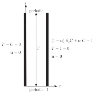
We consider a binary fluid mixture confined in a two-dimensional vertically extended container with the two opposite sidewalls, at x = 0,ℓ∗_{, maintained at prescribed (and unequal) temperatures} and concentrations (Fig. 1). We adopt periodic boundary conditions in the z direction with spatial period H∗, and denote the dimensionless aspect ratio by Ŵ ≡ H∗/ℓ∗. We suppose that the wall at x = 0 is maintained at a constant temperature T_r∗ and concentration C_r∗ while along the wall x = ℓ∗ the temperature is maintained at Tr+1T∗ with 1T∗ >0. Along this wall we apply a Robin type boundary condition on the concentration C∗: (1 − α)∂xC∗+αC∗ ≡Cr+1C∗. When no convection is present, this condition describes a wall that is maintained at a constant concentration Cr +1C∗ with 1C∗ >0. In the presence of convection, however, the concentration gradient near the sidewall steepens resulting in a concentration difference 1C∗ _{across the system that increases} with the Grashof number, defined below. A boundary condition of this type corresponds to a semipermeable wall at x = ℓ∗ _{that allows solute to seep into the interior 0 < x < ℓ}∗ _{from a solute} reservoir in x > ℓ∗_{. In particular, when α = 1 the right sidewall is completely permeable and the} interior is then in full contact with the solute bath outside.

We use the Boussinesq approximation with the fluid density ρ given by ρ = ρ0+ρT(T∗−Tr∗) + ρC(C∗−Cr∗), where T∗and C∗are, respectively, the (dimensional) temperature and concentration, and ρT <0 and ρC >0 are the thermal and solutal expansion coefficients at the reference temperature

T _{= C = 0} u_{= 0} u_{= 0} T −1 = 0 (1 − α) ∂xC_{+ α C = 1} x z Γ periodic 1 periodic

FIG. 1. Sketch of the geometry indicating the assumed dimensionless boundary conditions. T∗

r and concentration Cr∗. The Soret and Dufour (cross-diffusion) effects are ignored. Using ℓ∗_{, ℓ}∗2_/ν∗_{, ν}∗_/ℓ∗_{, 1T}∗_{, and 1C}∗_{as units of length, time, velocity, temperature difference T}∗_−T∗

r , and concentration difference C∗_−C∗

r, the dimensionless equations read

∂tu + (u · ∇)u = −∇p + ∇2u + Gr(T + N C)ez, (1) ∂tT +(u · ∇)T = Pr−1∇2T , (2)

∂tC +(u · ∇)C = Sc−1∇2C, (3)

∇ · u = 0, (4)

where u ≡ (u,w), ∇ ≡ (∂x,∂z) in the now dimensionless (x,z) coordinates, with x in the horizontal direction and z in the vertical direction. The Prandtl number Pr, the Schmidt number Sc, the Grashof number Gr, and the buoyancy ratio N are defined by Pr = ν∗/κ∗,Sc = ν∗/D∗,Gr = g∗|ρT|1T∗ℓ∗3/ρ0ν∗2, and N = −ρC1C∗/|ρT|1T∗, respectively. Here g∗is the acceleration due to gravity. The domain is Ŵ-periodic in the z direction, and the boundary conditions along the vertical walls read

x =0 : T = C = u = w = 0, (5)

x =1 : T − 1 = (1 − α)∂xC + αC −1 = u = w = 0, (6) where α ∈ [0,1] is a real parameter. The results that follow are computed for Sc = 11, Pr = 1, and N = −1. The problem then has the trivial solution u = 0, T = C = x for any value of the parameter α, and this solution is linearly stable up to a critical Grashof number that depends on the Lewis number Le = Sc/Pr, as well as on the parameter α and the aspect ratio Ŵ.

It is useful to rewrite the above equations in terms of the departures ˜T ≡ T − x and ˜C ≡ C − x from the conduction profile:

∂tu + (u · ∇)u = −∇p + ∇2u + Gr( ˜T − ˜C)ez, (7) ∂tT +˜ (u · ∇) ˜T = −u +Pr−1∇2T ,˜ (8) ∂tC +˜ (u · ∇) ˜C = −u +Sc−1∇2C,˜ (9)

subject to

x =0 : ˜T = ˜C = u = w = 0, (11)

x =1 : ˜T =(1 − α)∂xC + α ˜˜ C = u = w =0. (12) Equations (7)–(10) with the boundary conditions (11)–(12) are invariant under translations in the vertical, z → z + d, (u,w,p, ˜T , ˜C) → (u,w,p, ˜T , ˜C), with translations by multiples of Ŵ acting as the identity, as well as the reflection R1 : z → −z, (u,w,p, ˜T , ˜C) → (u, − w,p, ˜T , ˜C), with respect to an arbitrary origin z = 0. When α = 1 the equations also have a reflection symmetry in x: R2: x → 1 − x, (u,w,p, ˜T , ˜C) → (−u,w,p, ˜T , ˜C). The convecting state that sets in at the critical value of the Grashof number, Gr = Grc, is invariant under the double reflection R ≡ R1◦R2and is therefore stationary. When α 6= 1 the reflection symmetry R2 is broken and the convection pattern starts to drift, as described in [15]. The following section is devoted to understanding the properties of both stationary (α = 1) and drifting states (0 6 α < 1) in the strongly nonlinear regime.

III. NUMERICAL METHOD

We use a numerical arclength continuation method to follow both steady states and traveling waves (steady states in a moving frame). The equations are discretized in space using a spectral element method in which the domain is decomposed in the vertical direction into neequal spectral elements of size nx×nz. In each element, the fields are approximated by a high-order interpolant through the Gauss-Lobatto-Legendre points. Our numerical continuation method is based on a Newton solver for the time-independent version of the equations (and boundary conditions) written in a frame moving with velocity c. The unknowns include the velocity, temperature and concentration at the grid points, the Grashof number Gr and the wave velocity c. The Jacobian itself is never computed but its action on a given vector as well as the evaluation of the right-hand side at each Newton step follow Mamun and Tuckerman [16] as described elsewhere [5,7,8,17]. When calculating a traveling wave solution, an additional equation that fixes the phase must be added:

Z Ä

[(u − u†)∂zu†+(w − w†)∂zw†+(T − T†)∂zT†+(C − C†)∂zC†]dÄ = 0, (13) where Ä = [0,1]×[0,Ŵ] and the † indicates a previously calculated solution along the current solution branch. This solution can be updated during continuation. Finally, the linear stability of the solutions obtained in the continuation process is calculated using the Arnoldi method as described in Ref. [16]. More details on the code and its adaptation to other problems arising in fluid dynamics can be found in Refs. [7,17–19].

IV. RESULTS

A. The symmetric case: α = 1

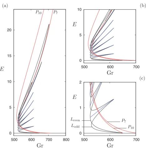
Figure2shows the bifurcation diagram computed using numerical continuation of steady states when α = 1, Ŵ = 10λc. Here λc = 2.513 is the approximate wavelength of the state that first sets in in an infinite system, as the Grashof number increases through Grc ≈ 650.937. The steady states come in two types, spatially extended states and spatially localized states. The former correspond to periodic convection and in the present case consist of 10 pairs of stationary inclined corotating rolls, hereafter referred to as P10. In the following we refer to the critical Grashof number as Gr10, Gr10 ≈ 650.937, since steady states with a different number of roll pairs also bifurcate from the conduction state, albeit for Gr > Gr10. The figure shows that this primary bifurcation is strongly subcritical and is therefore accompanied by a saddle-node bifurcation at Gr ≈ 516.77. We mention that the primary bifurcation generates a pattern with 10 pairs of counterrotating rolls. However, as one proceeds along the P10 branch the clockwise rolls within each roll pair rapidly weaken and shrink to zero, leaving a set of 10 counterclockwise rolls within the domain that gradually strengthen as one proceeds up the branch.

0 5 10 15 20 (a) (b) (c) 500 600 700 800 E Gr 0 5 10 500 600 700 0 1 2 500 600 700 Gr Gr E E P7 P10 P7 P10 Leven Lodd

FIG. 2. (a) Bifurcation diagram showing the kinetic energy E ≡ 1₂R₀ŴR₀1 u2_+w2_{dx dzalong the P} 10, P7, Lodd, and Levenbranches of stationary solutions as a function of the Grashof number Gr when α = 1, Ŵ = 10λc. The branch E = 0 shown in black corresponds to the conduction state and is stable up to Gr10 ≈ 650.937, where a subcritical bifurcation to a branch of 10 pairs of counterrotating rolls takes place. The clockwise rolls fade away as one proceeds up the corresponding P10 branch, leaving a state with 10 counterclockwise rolls. Along this branch, a secondary bifurcation takes place at Gr ≈ 648.466 producing a pair of snaking branches of spatially localized states (black curves). These branches terminate at a secondary bifurcation at Gr ≈ 581.183 located on the branch P7 of periodic states that bifurcates from the conduction state at Gr7 ≈ 715.54. The branches in blue indicate the so-called rung solutions and correspond to drifting asymmetric localized states. (b) A closer view of the snaking region. (c) Zoom of the lower part of the snakes-and-ladders structure of the snaking region.

As expected on the basis of general theory [11,20] the bifurcation to the periodic state is accompanied by a pair of branches of spatially localized states that bifurcate from the periodic state at a very small amplitude (Gr ≈ 648.466), and likewise subcritically. This bifurcation moves to lower and lower amplitude as the domain size grows and approaches Gr10 in the limit of infinite domains. The localized states exhibit snaking within a substantial interval of Grashof numbers, as described elsewhere [8], wherein the spatially localized states grow in spatial extent by successively adding pairs of rolls, one roll at either end. This growth process terminates when the available domain is full; in the present case the wavelength of the rolls within these isolated structures is larger than the wavelength λcof the periodic state with the result that the localized states terminate at Gr ≈ 581.183 on branch P7 consisting of seven corotating rolls within the domain. The two branches of localized states are intertwined and accompanied by interconnecting branches of traveling unstable asymmetric states shown in blue that extend from a fold on one branch to the corresponding fold on the other. In the theory these states correspond to the rungs of the so-called snakes-and-ladders structure [9] of the solutions within the snaking region.

Figures 3and 4show details of the two snaking branches, while Fig. 5shows sample solutions along the first rung of asymmetric states. Figure 3shows the branch (in bold) of localized states

0 5 10 15 20 25 500 600 700 E Gr ❅ ❅ ❅ L_odd

FIG. 3. The snaking branch Lodd with an odd number of rolls (bold, left panel) and the corresponding solutions shown at successive saddle nodes (right panels). The rightmost solution is the periodic solution at the termination point of Loddon P7. Parameters: α = 1, Ŵ = 10λc.

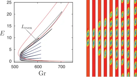
with an odd number of convection rolls, hereafter Lodd, while Fig.4shows the branch of localized states with an even number of rolls, hereafter Leven. In each case the panels on the right show the solution, appropriately centered, at successive folds on the snaking branch. All the rolls rotate counterclockwise. Note that the rolls at the right folds are more vigorous than those at the left folds and that the nucleation of new rolls takes place near the left folds. Both branches bifurcate together from P10 and terminate together on P7with seven rolls in the domain.

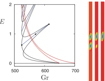
Figure 6shows the individual rungs of the snakes-and-ladders structure. Since the rungs form via pitchfork bifurcations from a circle of stationary states (i.e., via parity-breaking bifurcations at either end), each rung branch consists of a pair of asymmetric states, traveling in opposite directions. The speed c drops to zero as the square root of distance from either end, thereby forming an oval structure in the c(Gr) plots shown on the right; the narrowest states drift the fastest.

However, despite its richness the bifurcation diagram in Fig. 2 is incomplete. Figure 7 shows a more complete diagram showing a secondary branch of stationary states, referred to as M5, that bifurcates from P10 at higher amplitude (Gr ≈ 626.7). The states on this branch are so-called mixed modes and near Gr = 626.7 these resemble the 10-roll state with a superposed modulation

0 5 10 15 20 25 500 600 700

E

Gr

FIG. 4. The snaking branch Leven with an even number of rolls (bold, left panel) and the corresponding solutions shown at successive saddle nodes (right panels). The rightmost solution is the periodic solution at the termination point of Leven on P7. Parameters: α = 1, Ŵ = 10λc.

0 1 2 500 600 700

E

Gr

FIG. 5. Closeup of the first rung of the snakes-and-ladders structure of the snaking region (left panel). Solutions on the right correspond (from left to right) to Gr = 524.52, 570.09, and 614.63. The asymmetric states on the rung take the form of traveling pulses whose speed decreases to zero at either end of the branch where the reflection symmetry R is restored. Parameters: α = 1, Ŵ = 10λc.

with wavelength 2λc, i.e., this secondary bifurcation corresponds to a 2:1 spatial resonance. With increasing distance along the branch the contribution from the 10-roll state decreases rapidly with the result that the five-roll state dominates. We show sample profiles along this branch in panels 1–4 of Fig.7(c). We emphasize in particular the increasing length of each roll within the resulting M5 state as Gr increases, and the splitting of its core that takes place near the fold labeled 3 in Fig. 7(a). Near the energy maximum of M5 there is a tertiary parity-breaking bifurcation that leads to a traveling 5-roll state. Panel 5 in Fig. 7(c)shows a snapshot of an upward-traveling wave of this type; the asymmetry associated with a nonzero speed is manifest. Figure 8 shows that, as expected from a parity-breaking bifurcation, the speed varies as the square root of the distance from the bifurcation point in the vicinity of Gr = 695.2. Both this state and the related TW6 state identified below are unstable.

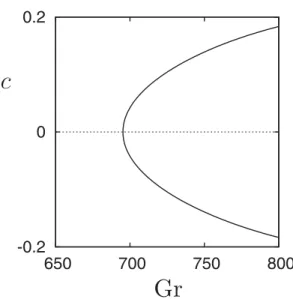
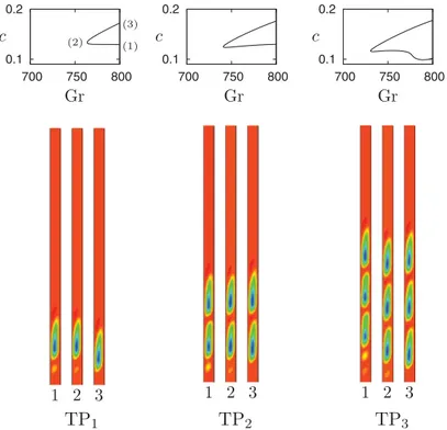
We now turn to the disconnected states labeled TPnin Fig. 7(a). These states correspond to spatially localized traveling pulses of convection, with TPnconsisting of a group of n corotating rolls within the domain, all traveling with the same speed. Figure 9shows the speed of the single-roll state TP1 as a function of the Grashof number Gr. In the figure states with c > 0 travel downward while those with c < 0 travel upward. Figure 10 shows the speeds c for downward-traveling TPn, n = 1,2,3, in each case with the corresponding solution profiles at the three locations indicated in the top left panel. Upward-traveling pulses are obtained by applying the symmetry R1 to each profile (Fig. 9). The rolls comprising each pulse are largely similar, despite an expected asymmetry between the fore and aft fronts that connect each structure to the background conduction state. In these plots states labeled 1 have larger energy than states labeled 3, a consequence of the small amplitude precursor that travels in front of the pulse and with the same speed. Thus at fixed Gr higher energy states move more slowly than lower energy states. The precursor itself develops in the vicinity of the fold and is associated with the growing asymmetry between the fore and aft fronts as the energy of the pulse grows along the higher energy branch. Along this branch the speed decreases slightly with increasing Gr (and hence increasing energy) while the opposite is the case for the TP1 states on the lower energy branch whose speed increases with increasing Gr (Fig. 10, top left panel). However, this straightforward behavior does not generalize to the TP2 and TP3 states (Fig. 10, top right panels).

Figures 7 and 10, computed for Ŵ = 10λc, suggest that the localized traveling pulses can be viewed as finite segments of a periodic traveling wave state. As a result we view the traveling pulses as accumulating on a heteroclinic cycle (in the comoving frame) consisting of an infinite TW segment connected fore and aft to the background conduction state. Figure 11provides further evidence for this view; in the figure, computed for Ŵ = 12λc, the TPnstates appear to converge

0 5 10 (a) (b) 500 550 600 650 -0.003 0 0.003 500 550 600 650 E Gr Gr c

FIG. 6. (a) Bifurcation diagram showing the kinetic energy E in the comoving frame, restricted to the rung states and the conduction state. (b) The speed c along each rung branch. Since the rungs form via parity-breaking bifurcations from circles of stationary states at either end, each rung branch consists of a pair of asymmetric states, traveling in opposite directions. Parameters: α = 1, Ŵ = 10λc.

on the TW states as n → ∞. Such finite traveling pulses form whenever the speeds of the fore and aft fronts coincide. However, the speeds of these fronts are expected to be unequal (owing to the absence of the reflection symmetry R1 for moving structures), requiring the presence of a 1:1 resonance between the speeds in order to obtain a bound state of two such fronts, i.e., a traveling pulse state that travels with a single speed. Imposing this requirement leads to a nonlinear eigenvalue problem for c(Gr), as reported in Fig.10. For further discussion of finite trains of traveling pulses see Ref. [21].

We have also determined the linear stability of the traveling pulse states identified in Figs.7and 11. In both cases these states were found to be unstable, in agreement with the instability of the TW state determined earlier. However, stable traveling states can be found when α < 1 as described next.

B. The nonsymmetric case: α < 1

We now turn to the case α < 1 corresponding to broken R2 symmetry. We first examine the effects of weak symmetry-breaking (α ≈ 1). Because of the loss of R2 symmetry all the steady solutions we have computed for α = 1, both periodic and spatially localized, now travel. This loss of symmetry results in the breakup of the α = 1 snakes-and-ladders structure of the snaking region into a stack of isolas, exactly as in the Swift-Hohenberg equation with broken reversibility [22]. The breakup into isolas is a consequence of the reconnection between the steady states that now travel and the rung states that travel because they were already asymmetric (Fig. 12). The mixed modes M5 likewise travel and reconnect with the TW branch which now splits into two distinct branches, one of upward-traveling waves and the other of downward-traveling waves (Fig. 12). Thus the loss of the R2 symmetry generates a multitude of traveling states, both extended and localized.

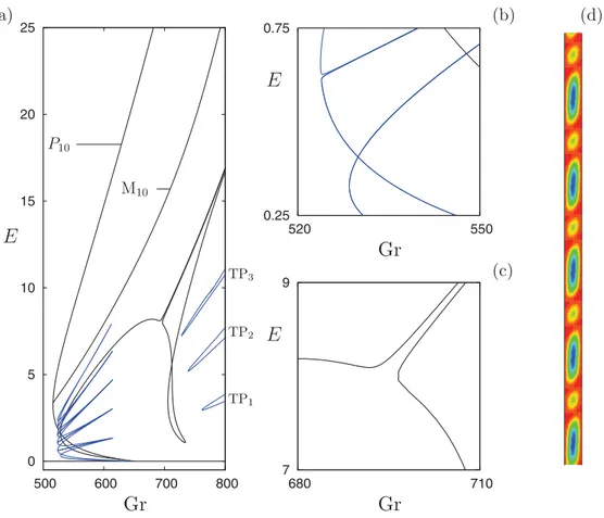
0 5 10 15 20 25 (a) (b) (c) 500 600 700 800 E Gr 0 0.5 1 500 600 700 800 1 2 3 4 5 M5 • 1 • 2 • 3 • 5 ❊ ❊ ❊ ❊ ❊ ❊ ❊ ❊ ❊ ❊ ❊ ❊ ❊ ❊ ❊ ❊ ❊❊ TW5 ❊ ❊ ❊ ❊ ❊ ❊ ❊ ❊ ❊ ❊ ❊ ❊ ❊ ❊ ❊ ❊ ❊❊ M5 • 4 Gr E TP1 TP2 TP3

FIG. 7. (a) A more complete bifurcation diagram showing an additional secondary branch of stationary solutions that bifurcates subcritically from P10 at Gr = 626.7 [panel (b)], producing a branch M5 of five corotating rolls [solution profiles 2–4 in panel (c)]. Along M5there is a tertiary bifurcation producing a branch of traveling periodic solutions (TW5, in blue), profile 5 in (c). Both up and down traveling states have identical energy and so appear as a single branch in the figure (the figure shows the kinetic energy in the comoving frame). Three additional disconnected branches of unstable traveling pulses (labeled TPn, n =1,2,3) are also shown. Parameters: α = 1, Ŵ = 10λc. -0.2 0 0.2 650 700 750 800

c

Gr

FIG. 8. The speed c along the TW5branch created in the tertiary parity-breaking bifurcation identified in Fig. 7. Parameters: α = 1, Ŵ = 10λc.

-0.2 0 0.2 750 800

c

Gr

FIG. 9. Upward-traveling (c < 0) and downward-traveling (c > 0) single-roll pulses TP1corresponding to the folds in the left panel. For TP2and TP3the results are similar. Parameters: α = 1, Ŵ = 10λc.

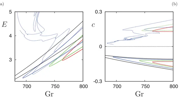
Figure 13(a) shows that as soon as α < 1 the branches of upward- and downward-traveling pulses also split, with the solid curves representing upward-traveling pulses and the broken curves representing downward-traveling pulses. The splitting becomes more prominent as α decreases and manifests itself in the behavior of the speed c shown in Fig. 13(b). The figure shows that the branch of downward-traveling pulses (dashed line) exhibits complex behavior already at α = 0.97. For α = 0.95 we have been unable to follow the downward-traveling pulses at all. In contrast, the upward-traveling pulses can be followed in α with no difficulty (solid line). The origin of this

0.1 0.2 700 750 800 0.1 0.2 700 750 800 0.1 0.2 700 750 800 Gr Gr Gr c c c (2) ₍₁₎ (3) 1 2 3 TP1 1 2 3 TP2 1 2 3 TP3

FIG. 10. Top panels: Wave speeds of the three disconnected downward-traveling pulses TPn shown in Fig.7. Bottom panels: Snapshots of the solutions at locations indicated in the top left panel. In each case the state labeled 1 has larger energy E than that labeled 3. Upward-traveling pulses are obtained by applying the symmetry R1 to each of the states shown. The figure suggests that the TPnstates, n = 1,2,3, can be viewed as finite segments of the domain-filling TW5 state. Parameters: α = 1, Ŵ = 10λc.

0 10 20 500 600 700 800

E

Gr

FIG. 11. Bifurcation diagram showing the kinetic energy E in the comoving frame as a function of the Grashof number Gr for α = 1, Ŵ = 12λc for comparison with Fig. 7. The traveling pulses TPn,1 6 n 6 4, persist (side panels) but remain unstable. The figure emphasizes that the TPn states can be viewed as finite segments of a domain-filling TW state, here TW6.

0 5 10 15 20 25 (a) (b) (c) (d) 500 600 700 800 E Gr 0.25 0.75 520 550 7 9 680 710 Gr Gr E E TP1 TP2 TP3 P₁₀ M10

FIG. 12. (a) Bifurcation diagram for α = 0.999, Ŵ = 10λc, showing the kinetic energy E as a function of the Grashof number Gr. All states now travel, and we use black curves to indicate spatially extended traveling states and blue curves to indicate spatially localized traveling states. Panels (b) and (c) show appropriate enlargements of panel (a) so that the reconnections within the snakes-and-ladders structure of the snaking region that take place as soon as α < 1 become (barely!) visible. An additional mixed mode state, labeled M10 and shown in panel (d), was omitted from Figs. 2and7in the interests of clarity but is included here for completeness. Like P10and P7(not shown) the M10state drifts as soon as α < 1.

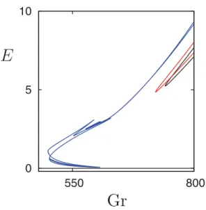
3 4 5 (a) (b) 700 750 800

E

c

r

G

r

G

FIG. 13. (a) The TP1 branches and (b) the corresponding speed c when α changes from α = 1 (red) to 0.99 (green), 0.97 (blue), and 0.95 (black) in a domain of aspect ratio Ŵ = 10λc. As soon as α < 1 the upward (continuous lines, c < 0) and downward (dashed lines, c > 0) traveling states split, resulting in behavior that depends on the direction of travel. We have been unable to follow the TP1 branch for downward-traveling pulses for α < 0.97.

behavior is unclear but is most likely associated with the inability of the fore and aft fronts to lock to one another, thereby destroying the localization responsible for the presence of the one-pulse state. Both fronts have natural speeds of propagation. These are equal and opposite when α = 1 owing to the presence of the center symmetry but become unequal as soon as α < 1. As a result one or other front depins more easily [22]. However, the overall motion of the TP1 state can reduce the overall speed difference thereby stabilizing the structure, or it can enhance it thereby leading to premature depinning and hence the absence of localized states altogether. We believe that this mechanism is responsible for the remarkable robustness of upward-traveling TP1 states and the corresponding fragility of downward-traveling TP1 states.

Figure14sheds additional light on this process. The figure shows the evolution of the branch of upward-traveling TP1 states with the parameter α in a global bifurcation diagram. The figure shows that as α decreases the region of existence of these states expands rapidly towards smaller values of the Grashof number [Fig. 14(a)] and reveals that for α ≈ 0.95 it connects with a second branch of traveling 1-pulses present at yet lower values of Gr [Fig. 14(b)]. This second branch originates in the breakup of the α = 1 snakes-and-ladders structure as explained above. Figure 14(c) shows the evolution of the resulting greatly extended TP1 branch as α decreases all the way to α = 0; cf. Ref. [23]. This figure is of interest since in the Swift-Hohenberg equation the isolas of traveling pulses shrink to zero as the equivalent of the parameter α decreases, and the traveling localized states disappear at finite α [22].

Figure 15 shows the corresponding reconnection behavior for TP2 as α decreases from α = 1 (black branch) to α = 0.99 (red branch) and then to α = 0.95 (blue branch). The figure shows that the reconnection process is now much more complex although its basic effect remains unchanged. The solution branch becomes more and more complex as α decreases further and we have not succeeded in following the solution branch in this regime. Yet more complex behavior appears to occur for TPn, n > 3.

Figure 16(a) provides an overview of the bifurcation diagram for α = 0 and Ŵ = 10λc, while Fig. 16(b) shows the TP1 branch in greater detail. The snapshots to the right show that at larger amplitudes the TP1 state is quite broad (profiles 1 and 5). It becomes quite localized as Gr decreases towards the left fold and then undergoes the nucleation of a precursor (profile 3), a transition that

0 2 4 500 600 (a) (b) (c) 700 800 0 2 4 500 600 700 800 0 5 10 300 550 800

E

Gr

E

Gr

E

Gr

FIG. 14. The kinetic energy E of the TP1 branch of upward-traveling pulses for (a) α = 0.97 and (b) α =0.95, both shown in red and superposed on the branches of steady and traveling states present for α = 1 (black dotted lines). (c) The kinetic energy E of the TP1branch over a much larger range of α: α = 1 (dotted), 0.9 (dashed), 0.5 (dashed-dotted), and 0 (solid). All solutions are computed for Ŵ = 10λc.

takes place in the vicinity of the lower right fold. Near the fold labeled 4 the precursor attaches to the main pulse, creating a broad localized structure that broadens yet more by location 5 on the branch. Figures 17(a) and 17(b)provide a detailed picture of the near-threshold behavior for this set of parameter values and in particular of the stability properties of TP1. Figure17(c) shows, in particular, that the primary bifurcation for this value of α is a supercritical Hopf bifurcation to a traveling wave state TW6 with six wavelengths within the domain. However, this state soon loses stability via a secondary Hopf bifurcation, i.e., a torus bifurcation. Figure 17(d) shows that the stable small amplitude TW6 states coexist with the detached branch of traveling pulses TP1, with the interval of stable pulses indicated by a heavy line. Comparison with Fig. 16(a)shows that the state TW8 is also stable in this regime. However, the stability region of TP1 does not overlap with that of TW7, a fact whose consequences are explored in the following section. Figure18shows the corresponding speeds c. 0 5 10 550 800

E

Gr

FIG. 15. Bifurcation diagram showing the TP2 branch for α = 1 (black), 0.99 (red), and 0.95 (blue) for comparison with Fig. 14.

0 1 5 10 350 450 550 650 750

E

Gr

E

Gr

FIG. 16. (a) Overview of the bifurcation diagram for α = 0, Ŵ = 10λc. Red lines refer to the traveling waves TW6, TW7and TW8shown in the panels on the right, with the filled triangles indicating secondary Hopf bifurcations. Note that TW7and TW8both acquire stability at larger amplitude. (b) Enlargement of the branch of the single-roll traveling pulses TP1showing the locations corresponding to the snapshots also shown on the right. 0 0.05 370 371 372 0 1 350 400 0 1 2 340 360 380 400 0 5 10 (a) (b) (d) (c) 300 550 800 E E E E Gr r G r G Gr TW7 TW6 TW8 TW7 TW6 TP1 TP1 TW8TW7 TW6 TP1

FIG. 17. (a) Bifurcation diagram showing the kinetic energy E as a function of Gr for α = 0 and Ŵ = 10λc with different enlargements shown in panels (b)–(d) with (c) and (d) including stability information. Panel (b) shows the detached branch of traveling pulses TP1 (black curve) while panel (d) indicates their stability: heavy continuous (light dotted) lines indicate stable (unstable) solutions. The TP1 lose stability at a Hopf bifurcation at Gr = 388.41 (thin vertical blue line). Filled triangles indicate this and other secondary Hopf bifurcations. Stable TP1 coexist with stable TW6 and stable TW8 but not with stable TW7; these traveling wave states (red curves) are created in successive primary Hopf bifurcations as shown in panels (c) and (d).

-0.1 0 0.25 0.5 (a) (b) 300 550 -0.5 0 0.5 300 550 800 c c r G r G TW8 TW7 TW6 TP1

FIG. 18. (a) Speed c as a function of Gr for α = 0 and Ŵ = 10λcalong the branches shown in Fig.17.

C. Direct numerical simulations for α = 0

In this section we describe the results of direct numerical simulations of Eqs. (1)–(4) with N = −1 and the boundary conditions (5)–(6) with α = 0 for Grashof numbers that straddle the loss of stability of the TP1state [Fig.17(d)]. Since α = 0 the symmetry R of the α = 1 system is strongly broken and upward and downward-traveling disturbances travel with very different speeds. Figure19(a)shows a stable upward-traveling TP1 state at Gr = 386.4 in a space-time diagram showing the vertical velocity w(x = 0.5,z,t) as a function of time, with time increasing towards the right. The pulse travels with speed c ≈ 0.086 in agreement with the speed computed from Newton iteration, with a compact but nonmonotonic leading front and an extended trailing tail. Figure 19(b)contrasts this behavior with that occurring at Gr = 390.4 (c ≈ 0.163), i.e., in the region just beyond the loss of stability of TP1at Gr ≈ 386.5. In this regime the TP1 state is predicted to be unstable, a prediction that is confirmed by the simulation. The simulation reveals that the unstable TP1 state evolves by emitting a small amplitude rapidly propagating precursor that extracts an ever-increasing amount of energy from the pulse, slowing it down, until such time as the pulse falls apart, generating a rapidly expanding region of spatio-temporal chaos. This turbulent state persists as time increases and is therefore apparently stable; in particular, there is no transition to any of the other stable states such as TW8 that coexist with this state. Figure 20(a) shows the chaotic state over a larger time interval. The figure shows a chaotic state consisting of rapidly traveling waves that intermittently collapses into a state consisting of one or more relatively long-lived slow-moving slugs of convection embedded in a laminar background that in turn breaks up into a chaotic state. The resulting lacunae

t t 0 Γ (a) (b) 5000 Γ 5000 z z 0

FIG. 19. Direct numerical simulations of the case α = 0 at (a) Gr = 386.4 (c ≈ 0.086) and (b) Gr = 390.4 (c ≈ 0.163) in a Ŵ = 10λcdomain, showing w(x = 0.5,z,t) in a space-time plot with time increasing to the right.

t t 5000 Γ (a) (b) (d) (c) 10000 Γ 10000 z z 9500 -0.5 0 0.5 0 0.25 -0.5 0 0.5 0 0.25 wm Em wm Em t t t t ₁₀₀₀₀ 0 0 0 0 1 0 0 0 0 1 10000 9500 9500 5000 5000

FIG. 20. (a) Continuation of the chaotic behavior in Fig. 19(b) for Gr = 390.4 on the time interval [5000,10 000]. (b) An enlargement of the region on the right of panel (a). Bottom panels show the corresponding time series of wm(t ) ≡ w(0.5,0.5Ŵ,t) and Em(t ) ≡ 1₂(u2m+w

2

m), where um(t ) = u(0.5,0.5Ŵ,t) over the time interval [5000,10 000] (left panels) and [9500,10 000] (right panels).

in the chaotic state may extend over a part of the domain or indeed the whole vertical extent of the domain. This unusual behavior resembles that associated with dispersive chaos [24,25] as well as the relaxation oscillations observed in binary fluid convection in a horizontal layer [26].

A detailed examination of Fig. 20(a)reveals that the chaotic state consists of several components that repeat in an intermittent and spatially aperiodic manner. These include relatively long-lived upward-drifting pulses of the type seen in Fig. 19(a) whose breakup recapitulates that shown in Fig. 19(b). These states emit low-amplitude, low-wave-number TW that travel downward with a speed that is substantially faster than that of the upward-drifting pulses [Fig. 20(b)]. The upward-drifting pulse ultimately starts to pulsate and turns into a larger amplitude traveling wave resembling TW7 that travels downward with speed close to the computed TW7 speed (c ≈ 0.0725). At this value of Gr the TW7 is barely unstable, with a growth rate 0.355×10−3, accounting for the relatively long time for which the solution resembles TW7 before departing from it. As a result the dynamics, in this part of the space-time plot at least, resemble a complex oscillation between three states, an upward-drifting spatially localized pulse state resembling TP1 and two different extended traveling wave states, both of which travel downward. Figure 18confirms that the pulse TP1 and the traveling waves TW7 do indeed have opposite speeds at this value of the Grashof number, Gr = 390.4, and given the trend revealed in Fig. 18(a) it is likely that the smaller wavelength waves present in the chaotic regime in Fig. 19(b)likewise have a downward phase velocity.

Figure20(b)shows that the lacunae that are interspersed throughout the chaotic state are in fact all filled with the small-amplitude traveling waves. This is as expected, given that the base state is unstable to traveling waves at this value of Gr. The lacunae are themselves generated in almost all cases by the same process: a rapid upward expansion of the void owing to the progressive collapse of a downward-traveling wave TW7, followed by a slower downward-moving front that closes the void with the TW7 speed. In other words, the voids are closed off by the invasion of the void by these

t t 5000 Γ 10000 (a) (b) Γ 8500 z z 7500

FIG. 21. (a) Transient chaotic behavior at Gr = 391 over the time interval [5000,10 000] initialized at t = 0 with an unstable TP1solution at Gr = 391. (b) An enlargement of the time interval [7500,8500] showing abrupt collapse of the chaotic state into a modulated traveling wave MTW4.

larger amplitude waves, and it is this invasion that determines their lateral extent. It is noteworthy that the process that opens the void conserves phase, i.e., no phase slips take place during this process [Fig.20(b)], indicating that the frequency and wavelength adjust to the falling amplitude in just the right way to maintain phase. Since the wavelength is approximately conserved [Fig. 20(b)] the ob-served change in phase speed can be ascribed to the change in oscillation frequency as the amplitude falls. This conclusion is consistent with the presence of folds in the TW branches shown in Fig. 18(a), a trend that is likely followed by the smaller wavelength TW present in the chaotic state. We conclude that the observed chaotic state is mediated by connections in phase space between upward-traveling localized pulses and downward-traveling TW of small and large amplitude but identical wavelength.

Thus far we have examined the dynamics in the “gap” between stable TP1 states and stable TW7 states. In Fig. 21(a) we examine what happens when Gr is increased to Gr = 391 at which the TW7 state is stable. The figure shows that rather than collapsing to the stable TW7 state the spatio-temporally chaotic state remains, albeit as a long transient. Moreover, this state collapses to a new state, a periodically modulated TW4 state, hereafter MTW4. This is a two-frequency state, with one frequency corresponding to drift and the other to the temporal modulation, and appears to be stable. This statement is consistent with the observation that the kinetic energy E(t) is a single frequency oscillation (not shown). It follows that the TW7 is not part of the spatio-temporally chaotic attractor at Gr = 390.4, and that the collapse to MTW4 occurs spontaneously because the instability of this state manifests itself at a phase when the state is not close to a TW7 state [Fig. 21(b)]. We surmise that if the instability manifests itself during a different phase of the oscillation the final outcome might be different, for example, resulting in a collapse to the now stable TW7 state. These observations suggest that the collapse of the spatio-temporally chaotic state is unrelated to the change of stability of TW7 but that it is nevertheless highly complex, with extreme sensitivity to initial conditions. Detailed exploration of this transition is beyond the scope of this work, however.

V. CONCLUSIONS

In this paper we have studied the properties of stationary and traveling states in natural doubly diffusive convection in the so-called opposing case, i.e., when the temperature and solute gradients across the system balance and a stationary conduction state is present. Steady convecting states were found when the system possesses a reflection symmetry, in the present case a center symmetry. In this case we found, by explicit computation, that steady localized states are organized in a snakes-and-ladders structure familiar from studies of the bistable Swift-Hohenberg equation [20]. Since the equations are not variational the asymmetric localized states lying on the rungs of this

structure all drift; we were able to compute the drift speed by solving the corresponding nonlinear eigenvalue problem. One unexpected discovery was the presence of a branch of stationary mixed modes, referred to as M5, extending well outside the snaking region. This branch originates in a subsidiary secondary bifurcation from the primary branch of periodic states, and exhibits a parity-breaking bifurcation to traveling waves. The resulting traveling waves persist over a wide range of Grashof numbers and coexist with stable stationary convection. By employing homotopy methods, following earlier work by Beaume et al. [27] and Mercader et al. [23], we were able to identify a series of spatially localized traveling “pulses” that appear to accumulate on the branch of traveling waves. Detailed stability calculations revealed that these traveling states are in fact linearly unstable, at least for the parameter values explored. Despite this the important message of this paper remains that nongradient systems may exhibit a wide variety of disconnected spatially localized traveling states that may or may not be stable. We have described a procedure that allows one to identify such states, a homotopy method that allows one to latch onto these solutions for one set of boundary conditions, followed by continuation back to the desired boundary conditions.

As part of the homotopy procedure we have explored the consequences of progressively breaking the center symmetry of the system by decreasing the homotopy parameter α (a Biot number of the right wall) away from the value α = 1 required for center symmetry. As expected, once α < 1 all stationary states drift. However, in addition, a number of reconnections with the drifting states present already for α = 1 take place, leading to the generation of traveling pulses over a wide range of values of the Grashof number, some of which are now stable. Explicit stability calculations, corroborated by direct numerical simulations, identified parameter regimes with such stable traveling pulses. While the details of the mathematical origin of these pulses remain to be fully understood (Ref. [28] may be helpful), it is evident that the dynamics of natural doubly diffusive convection are much more complex than existing studies indicate. In fact, the states we have computed are of a rather simple type: they are stationary states or equilibria in an appropriately moving frame. It is known, however, that in systems in which the primary bifurcation is a subcritical Hopf bifurcation to extended traveling waves, one typically finds localized traveling waves as well. These states are of an altogether different type, being quasiperiodic in time: the wave travels with phase speed cpthrough an envelope that moves with the group speed cg 6= cp. States of this type are expected to be present in the system studied here once α differs from α = 1 sufficiently so that the Hopf frequency is no longer small but are much harder to compute numerically [14]. We propose to investigate quasiperiodic localized traveling waves and the quasiperiodic spatially extended MTW states identified in the previous section in future work.

Finally, we have used direct numerical simulation to determine the dynamics of the system when the localized traveling pulses lose stability. These calculations, performed for α = 0, i.e., fixed concentration flux on the right wall, revealed complex dynamics at quite small amplitude. This behavior, characterized by strong intermittency, coexists with stable large amplitude traveling wave convection. We have presented numerical evidence suggesting that at least some aspects of this behavior may be understood in terms of switching between three competing states: slow upward-drifting convection pulses and two classes of spatially extended downward-traveling waves. However, owing to the relatively large aspect ratio of the system the switching does not take place synchronously throughout the computational domain and occurs instead in patches, leading to the observed spatio-temporal intermittency.

ACKNOWLEDGMENTS

This work was supported in part by the National Science Foundation under Grant No. DMS-1613132. We acknowledge helpful discussions with C. Beaume.

[1] T. Radko, Double-diffusive Convection (Cambridge University Press, Cambridge, 2013).

[2] W. R. Wilcox, Transport phenomena in crystal growth from solution,Prog. Cryst. Growth Charact. 26, 153(1993).

[3] K. Ghorayeb and A. Mojtabi, Double diffusive convection in a vertical rectangular cavity,Phys. Fluids 9, 2339(1997).

[4] S. Xin, P. L. Quéré, and L. S. Tuckerman, Bifurcation analysis of double-diffusive convection with opposing horizontal thermal and solutal gradients,Phys. Fluids 10,850(1998).

[5] A. Bergeon and E. Knobloch, Periodic and localized states in natural doubly diffusive convection, Physica D (Amsterdam) 237,1139(2008).

[6] A. Bergeon and E. Knobloch, Natural doubly diffusive convection in three-dimensional enclosures, Phys. Fluids 14,3233(2002).

[7] C. Beaume, A. Bergeon, and E. Knobloch, Convectons and secondary snaking in three-dimensional natural doubly diffusive convection,Phys. Fluids 25,024105(2013).

[8] A. Bergeon and E. Knobloch, Spatially localized states in natural doubly diffusive convection,Phys. Fluids 20,034102(2008).

[9] J. Burke and E. Knobloch, Localized states in the generalized Swift-Hohenberg equation,Phys. Rev. E 73,056211(2006).

[10] M. Nagata, Three-dimensional finite-amplitude solutions in plane Couette flow: Bifurcation from infinity, J. Fluid Mech. 217,519(1990).

[11] A. Bergeon, J. Burke, E. Knobloch, and I. Mercader, Eckhaus instability and homoclinic snaking, Phys. Rev. E 78,046201(2008).

[12] P. Kolodner, C. M. Surko, and H. Williams, Dynamics of traveling waves near the onset of convection in binary fluid mixtures,Physica D (Amsterdam) 37,319(1989).

[13] W. Barten, M. Lücke, M. Kamps, and R. Schmitz, Convection in binary fluid mixtures. II. Localized traveling waves,Phys. Rev. E 51,5662(1995).

[14] T. Watanabe, M. Iima, and Y. Nishiura, Spontaneous formation of travelling localized structures and their asymptotic behaviour in binary fluid convection,J. Fluid Mech. 712,219(2012).

[15] R. E. Ecke, F. Zhong, and E. Knobloch, Hopf bifurcation with broken reflection symmetry in rotating Rayleigh-Bénard convection,Europhys. Lett. 19,177(1992).

[16] C. K. Mamun and L. S. Tuckerman, Asymmetry and Hopf bifurcation in spherical Couette flow, Phys. Fluids 7,80(1995).

[17] C. Beaume, A. Bergeon, H.-C. Kao, and E. Knobloch, Convectons in a rotating fluid layer,J. Fluid Mech. 717,417(2013).

[18] D. L. Jacono, A. Bergeon, and E. Knobloch, Magnetohydrodynamic convectons,J. Fluid Mech. 687,595 (2011).

[19] D. L. Jacono, A. Bergeon, and E. Knobloch, Three-dimensional spatially localized binary-fluid convection in a porous medium,J. Fluid Mech. 730,R2(2013).

[20] E. Knobloch, Spatial localization in dissipative systems,Annu. Rev. Condens. Matter Phys. 6,325(2015). [21] A. Yochelis, E. Knobloch, and M. H. Köpf, Origin of finite pulse trains: Homoclinic snaking in excitable

media,Phys. Rev. E 91,032924(2015).

[22] J. Burke, S. M. Houghton, and E. Knobloch, Swift-Hohenberg equation with broken reflection symmetry, Phys. Rev. E 80,036202(2009).

[23] I. Mercader, O. Batiste, A. Alonso, and E. Knobloch, Travelling convectons in binary fluid convection, J. Fluid Mech. 722,240(2013).

[24] C. S. Bretherton and E. A. Spiegel, Intermittency through modulational instability,Phys. Lett. A 96,152 (1983).

[25] H. Chaté, Spatiotemporal intermittency regimes of the one-dimensional complex Ginzburg-Landau equation,Nonlinearity 7,185(1994).

[26] O. Batiste, E. Knobloch, A. Alonso, and I. Mercader, Spatially localized binary fluid convection,J. Fluid Mech. 560,149(2006).

[27] C. Beaume, H.-C. Kao, E. Knobloch, and A. Bergeon, Localized rotating convection with no-slip boundary conditions,Phys. Fluids 25,124105(2013),

[28] A. R. Champneys, V. Kirk, E. Knobloch, B. E. Oldeman, and J. D. M. Rademacher, Unfolding a tangent equilibrium-to-periodic heteroclinic cycle,SIAM J. Appl. Dyn. Syst. 8,1261(2009).