HAL Id: emse-00805114
https://hal-emse.ccsd.cnrs.fr/emse-00805114
Submitted on 21 Jan 2019
HAL is a multi-disciplinary open access
archive for the deposit and dissemination of
sci-entific research documents, whether they are
pub-lished or not. The documents may come from
teaching and research institutions in France or
abroad, or from public or private research centers.
L’archive ouverte pluridisciplinaire HAL, est
destinée au dépôt et à la diffusion de documents
scientifiques de niveau recherche, publiés ou non,
émanant des établissements d’enseignement et de
recherche français ou étrangers, des laboratoires
publics ou privés.
Dynamic Design Space Partitioning for Optimization of
an Integrated Thermal Protection System
Diane Villanueva, Rodolphe Le Riche, Gauthier Picard, Raphael Haftka
To cite this version:
Diane Villanueva, Rodolphe Le Riche, Gauthier Picard, Raphael Haftka.
Dynamic
De-sign Space Partitioning for Optimization of an Integrated Thermal Protection System.
54th
AIAA/ASME/ASCE/AHS/ASC Structures, Structural Dynamics, and Materials Conference, Apr
2013, Boston, United States. �10.2514/6.2013-1534�. �emse-00805114�
Dynamic Design Space Partitioning for Optimization of an
Integrated Thermal Protection System
Diane Villanueva
1,2∗, Rodolphe Le Riche
2,3†, Gauthier Picard
2‡,
and Raphael T. Haftka
1§1University of Florida, Gainesville, FL, 32611, USA
2Ecole Nationale Sup´erieure des Mines de Saint- ´´ Etienne, Saint- ´Etienne, France 3CNRS LIMOS UMR 6158
In this paper, we explore the use of design space partitioning to tackle optimization problems in which each point is expensive to evaluate and there are multiple local optima. The overarching goal of the method presented in this paper is to locate all local optima rather than just the global one. Locating multiple designs provides insurance against discovering that late in the design process a design is poor due to modeling errors or overlooked objectives or constraints. The proposed strategy to locate multiple candidate designs dynam-ically partitions the search space among several “agents” that approximate their sub-region landscape using surrogates. Agents coordinate by exchanging points to form an approximation of the objective function or constraints in the sub-region and by modifying the boundaries of their sub-sub-regions. Through a self-organized process of creation and deletion, agents adapt the partition as to exploit potential local optima and explore un-known regions. This idea is demonstrated on a six-dimensional analytical function, and a practical engineering example, the design of an integrated thermal protection system.
Nomenclature
c = center
f = objective function
F = objective function values associated with design of experiments in database
g = constraint
G = constraint values associated with design of experiments in database
t = time
x = design variables
X = design of experiments in database
ˆ
f = surrogate prediction of f
ˆg = surrogate prediction of g
I.
Introduction
Many contemporary applications can be modeled as distributed optimization problems (ambient intelligence, machine-to-machine infrastructures, collective robotics, complex product design, etc.). Optimization processes iteratively choose new points in the search space and evaluate their performances until a solution is found. However, a practical and common difficulty in optimization problems is that the evaluations of new points require expensive com-putations. For instance, if one wants to compute a property of a complex object (e.g. large deflections of an aircraft wing under some loading), a high fidelity computation (e.g. finite element analysis) may be required. Therefore, many
∗Graduate Research Assistant, Mechanical and Aerospace Engineering/Institut Henri Fayol, AIAA student member †CNRS permanent research associate, Institut Henri Fayol
‡Associate Professor, Institut Henri Fayol
researchers in the field of optimization have focused on the development of optimization methods adapted to expen-sive computations. The main ideas underlying such methods are often the use of surrogates, problem decomposition, and parallel computation. The use of surrogates to replace expensive computations and experiments in optimization
has been well documented.1,2,3,4 Moreover, in optimization, a common way to decompose problems is to partition
the search space.5,6 Furthermore, to take advantage of parallel computing, many have proposed strategies for using
multiple surrogates in optimization.7,8,9,10 The goal of most of these algorithms is to locate the global optimum, while
trying to minimize the number of calls to the expensive functions. Like these algorithms, we try to reduce the number the number of calls to the expensive functions, but our main goal is to locate multiple optima as multiple candidate designs. For real-world problems, the ability to locate many optima in a limited computational budget is desirable as the global optimum may be too expensive to find, and because it provides the user with a diverse set of acceptable solutions as insurance against late formulation changes (e.g., new constraints) in the design process.
Besides the aforementioned techniques for distributing the solving process, multi-agent optimization is an active
research field proposing solutions for distinct agents to cooperatively find solutions to distributed problems.11 They
mainly rely on the distribution (and decomposition) of the formulation of the problem. Generally, the optimization framework consists of distributing variables and constraints among several agents that cooperate to set values to
vari-ables that optimize a given cost function, like in the DCOP model.12 Another approach is to decompose or transform
problems into dual forms that can be solved by separate agents13 (for problems with specific properties, such as
lin-earity).
Here, we describe a multi-agent method in which the search space is dynamically partitioned (and not the problem formulation) into sub-regions in which each agent evolves and performs a surrogate-based continuous optimization. The novelty of this approach comes from the joint use of (i) surrogate-based optimization techniques for expensive computation and (ii) self-organization techniques for partitioning the search space and finding all the local optima. Coordination between agents, through exchange of points and self-organized evolution of the sub-region boundaries
allows the agents to stabilize around local optima. Like some nature-inspired niching methods,14,15 such as particle
swarm16,17,18and genetic algorithms,19,20or clustering global optimization algorithms,21our goal is to locate multiple
optima, but unlike these algorithms, our approach aims to sparingly call the true objective function and constraints. Our multi-agent approach further (i) uses the creation of agents for exploring the search space and, (ii) merges or deletes agents to increase efficiency.
In the following section, we discuss more deeply the motivation for multiple candidate designs. Next, we provide
some background on surrogate-based optimization. In Sec.IV, we describe the autonomous agents that perform the
cooperative optimization process. In Sec.V, we present the methods of space partitioning and point allocation that
are intended to distribute local optima among the partitions while maximizing the accuracy of the surrogate in a
self-organized way – through agent creation and deletion. In Sec. VIa six-dimensional problem is tackled using our
multi-agent optimizer, and in Sec.VIIa practical engineering example, the design of an integrated thermal protection
system, is presented.
II.
Motivation for Multiple Candidate Designs
In optimization courses, we often tell students that defining an optimization problem properly is the most important step for obtaining a good design. However, even experienced hands often overlook important objective functions and constraints. There are also epistemic uncertainties, such as modeling errors, in the objective functions and constraints definitions that will typically perturb their relative values throughout the design space. In one case, Nagendra et
al.19 used a genetic algorithm to find several structural designs with comparable weight and identical load carrying
capacity. However, when three of these designs were built and tested, their load carrying capacity was found to differ by 10%. For such reasons, alternative local optima may be better practical solutions to a given optimization problem than a single idealized global optimum. As advances in computer power have made it possible to move from settling on local optima to finding the global optimum, when designing engineering systems. This usually requires search in multiple regions of design space, expending most of the computation needed to define multiple alternate designs. Thus, focusing solely on locating the best design may be wasteful.
In engineering design, the simulated behavior of objective functions and constraints usually has modeling error, or epistemic uncertainty, due to the inability to perfectly model phenomena. Modeling errors can degrade local optima or even cause them to disappear.
Let us now turn to a practical engineering design example to demonstrate the presence, diversity, and fragility of candidate designs. Large portions of the exterior surface of many space vehicles are devoted to providing protection from the severe aerodynamic heating experienced during ascent and atmospheric reentry. A proposed integrated
thermal protection system (ITPS) provides structural load bearing function in addition to its insulation function and in
doing so provides a chance to reduce launch weight. Figure1displays the corrugated-core sandwich panel concept of
an ITPS, which consists of top and bottom face sheets, webs, and insulation foam between the webs and face sheets.
Figure 1. Integrated thermal protection system provides both insulation and load carrying capacity, and consequently can lead to alterna-tive optima of similar mass but different way of addressing the thermal and structural requirements.
The thermal and structural requirements often conflict due to the nature of the mechanisms that protect against the failure in the different modes. For example, thin webs prevent the flow of heat to the bottom face but are more susceptible to buckling and strength failure. A reduction in foam thickness (panel depth) improves resistance against buckling of the webs but increases heat flow. A thick bottom face sheet acts as a heat sink and reduces the temperature at the bottom face but increases stress in the web.
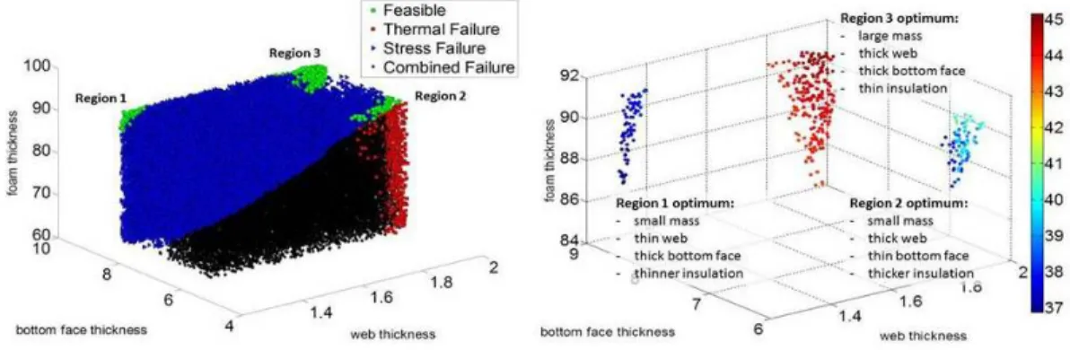
These conflicts may be resolved by candidate designs in different ways. Figure 2 displays the infeasible and
feasible regions with constraints on the temperature of the bottom face sheet and stress in the web for the three-dimensional example, in which the web, bottom face, and foam thicknesses were the design variables.
Figure 2. Feasible regions 1-3 and infeasible regions (left) and mass objective function represented by color (right). The two competitive optima in Regions 1 and 2 rely on different concepts. In Region 1 the thermal function is satisfied by a thick bottom face sheet acting as heat sink, while in Region 2 it is satisfied by thick insulation.
Three islands of feasibility are observed, in which the design is driven to protect against different failure modes. The two minimum mass designs are in Regions 1 and 2. In Region 1, the failure is primarily from stress, because the webs are thin. This is compensated by reducing the length of the web by reducing the foam thickness, and to compensate for the increase heat flow, the bottom face sheet is increased to provide a larger heat sink. In Region 2, both failure modes are present, so that the insulation is thicker to prevent thermal failure and the bottom face is thinner to reduce stress in the web. With both feasible regions being rather narrow, modeling errors can easily wipe out one of these regions, so that having both designs provides valuable insurance. Furthermore, even if modeling errors do not wipe out Region 2 but only narrow it, this can result in substantial increase in mass, while Region 1 is more robust.
This example demonstrates the benefit of multiple candidate designs due to the fragility designs from errors. In the following sections, the dynamic design space partitioning algorithm is described, and a six dimensional analytical
III.
Surrogate-Based Optimization
A surrogate is a mathematical function that (i) approximates outputs of a studied model (e.g. the mass or the strength or the range of an aircraft as a function of its dimensions), (ii) is of low computation cost and (iii) aims at
predicting new outputs.22 The set of initial candidate solutions, or points, used to fit the surrogate is called the design
of experiments (DOE). Known examples of surrogates are polynomial response surface, splines, neural networks or kriging.
Let us consider the general formulation of a constrained optimization problem, minimize
x∈S⊂ℜn f(x)
subject to g(x)≤ 0 (1)
In surrogate-based optimization, a surrogate is built from a DOE, denoted by X that consists of sets of the design variables x. For the design of experiments, there are the calculated values of the objective function f and constraints
gthat are associated with the DOE, which we denote as F and G, respectively. We will refer to X and its associated
values of F and G as a database.
The database is used to construct the surrogate approximation of the objective function ˆf and the approximation
of the constraint ˆg. We can approximate the problem in Eq.(1) using the surrogates and formulate the problem as
minimize x∈S⊂ℜn ˆ f(x) subject to ˆg(x)≤ 0 (2)
The solution to this approximate problem is denoted ˆx∗.
Surrogate-based optimization calls for more iterations to find the true optimum, and is therefore dependent on
some iteration time t. That is, after the optimum of the problem in Eq.(2) is found, the true values f ( ˆx∗) and g( ˆx∗) are
calculated and included in the DOE along with ˆx∗. At the next iteration, the surrogate is updated, and the optimization
is performed again. Therefore, we denote the DOE at a time t as Xt and the associated set of objective function
values and constraint values as Ftand Gt, respectively. The surrogate-based optimization procedure is summarized in
Algorithm1(which also refers to a global optimization procedure in Algorithm2).
Algorithm 1: Overall surrogate-based optimization t = 1 (initial state)
while t≤ tmaxdo
Build surrogates ˆf and ˆg from (Xt, Ft, Gt)
Optimization to find ˆx∗(see Algorithm2)
Calculate f ( ˆx∗) and g( ˆx∗)
Update database (Xt+1, Ft+1, Gt+1)∪ ( ˆx∗,f( ˆx∗), g( ˆx∗))
t = t +1
Algorithm 2: Constrained optimization procedure
input : ˆf ,ˆg, Xt, L output: ˆx∗ ˆx∗← argmin x∈L ˆ f(x) subject to ˆg(x)≤ 0
if ˆx∗is near Xtor out of the search domainL then
ˆx∗← argmax
x∈S
distance(Xt)
IV.
Agent Optimization Behavior
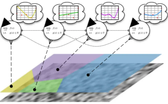
As stated in the introduction, our approach consists in splitting the space in sub-regions and assigning agents to
each of these sub-regions as presented in Fig.3. Therefore, Algorithm1can be thought of as the procedure followed
by a single agent to find one point, that will be repeating until termination. However, in the multi-agent approach
we describe here, each agent is restricted to only a sub-region of the design space, i.e.,S is replaced by a part of S.
smaller space, which we denote as Pifor the ith agent, and considers a simpler function. Each agent must consider
only the points in its sub-region, which are available in its internal database (Xt,F
t
,G
t
)i. The sub-region of an agent
is defined by the position of its center c. A point in the space belongs to the sub-region with the nearest center, where
the distance is the Euclidean distance. This creates sub-regions that are Voronoi cells.23 The choice of where to place
the center is discussed in the next section. Figure3illustrates the partition of a two-dimensional space into four
sub-regions for four agents, which requires four centers. In this example, we place the centers randomly. space partitions
will be discussed in SectionV.
min x∈S f (x) s.t. g(x)≤ 0 min x∈S f (x) s.t. g(x)≤ 0 min x∈S f (x) s.t. g(x)≤ 0 min x∈S f (x) s.t. g(x)≤ 0
Figure 3. Multi-agent System overview: agents perform surrogate-based optimization in different sub-regions of the partitioned search space based on personal surrogates (dashed l.) and exchange points with their direct neighbors (dotted l.)
The procedure of a single agent is given in Algorithm3. Assuming that sub-regions are defined, each agent fits
several surrogates it knows (as many different ways to approximate) and chooses the one that maximizes the accuracy in its sub-region (line 5-9). To avoid ill-conditioning, if more points are needed than are available to an agent, the agent asks neighboring agents for points. The neighboring agents then communicate the information associated with these points (lines 6–8). We define the best surrogate as the one with the minimum cross-validation error, the partial
prediction error sum of squares PRES SRMS. This is found by leaving out a point, refitting the surrogate, and measuring
the error at that point. The operation is repeated for p points in the agent’s sub-region (disregarding any points received
from other agents) to form a vector of the cross-validation errors eXV. The value of PRES SRMS is then calculated by
PRES SRMS = 1 pe T XVeXV (3)
Algorithm 3: Agent i optimization in its sub-region. 1 t = 1 (initial state)
2 while t ≤ tmaxdo
3 Update Pi = {x ∈ S s.t.||x − ci||2≤ ||x − cj||2, j i}
4 Update internal database from the new space partition
5 Build surrogates ˆf and ˆg from (Xt
,F
t
,G
t) i
6 if Not sufficient number of points in internal database to build a surrogate then
7 Get points from other agents closest to ci
8 Build surrogates
9 Choose best surrogate based on partial PRES SRMS error
10 Optimization to find ˆx∗[with Algorithm2( ˆf,ˆg,X
t ,Pi)] 11 Calculate f ( ˆx∗) and g( ˆx∗) 12 (Xt+1,Ft+1,Gt+1)i← (X t ,F t ,G t )i∪ ( ˆx∗,f( ˆx ∗ ),g( ˆx ∗ ))
13 Update center ci(see SectionA)
14 Check for merge, split or create (see SectionB)
15 t = t + 1
Once the agents have chosen surrogates (line 9), the optimization is performed to solve the problem in Eq.(2)
inside the sub-region (line 10). If the optimizer gives an infeasible point (i.e., the point does not satisfy the constraint
in the sub-region. To explore, the agent adds a point to the database that maximizes the minimum distance from the
points already in its internal database (see Algorithm2). The true values f and g of the iterate are then calculated (line
11), and ( ˆx∗,f( ˆx∗), g( ˆx∗)) is added to the internal database (lines 11–12).
V.
Dynamic Design Space Partitioning
The previous section expounds the cooperative optimization process performed by agents in a pre-partitioned space. The goal of this method is to have each agent locate a single optimum, such that the partitioning strongly depends on the topology of the space. Therefore, as a part of the cooperative optimization process, we propose a self-organizing mechanism to dynamically partition the space which adapts to the search space. By self-organizing, we mean that agents (and therefore sub-regions) will be created and deleted depending on the cooperative optimization process. Agents will split when points are clustered inside a single region (creation), and will be merged when local optima converge (deletion).
A. Moving the Sub-regions’ Centers
The method of space partitioning we propose focuses on moving the sub-regions’ centers to different local optima. As a result, each agent can choose a surrogate that is accurate around the local optimum, and the agent can also explore the sub-region around the local optimum. At the beginning of the process, only one agent exists and is assigned to the whole search space. Then it begins optimization by choosing a surrogate, fitting it and optimizing on this surrogate.
As a result the agent computes a new point ˆx∗t−1. Then, the center of the sub-region is moved to the “best” point in the
sub-region in terms of feasibility and objective function value (line 13). This is done by comparing the center at the
last iteration ct−1to the last point added by the agent ˆx∗t−1. The center is moved to the last point added by the agent if
it is better than the current center. Otherwise, the center remains at the previous center. For convenience, in comparing
two points xmand xn, we use the notation xm≻ xnto represent xm“is better than” xn. For two centers, instead of points
xwe would consider the centers c. The conditions to determine the better of two points are given in Algorithm4.
Algorithm 4: Algorithm to determinine if, for two points xmand xn, xm“is better than” xn(xm≻ xn) and vice
versa.
input : f (xm), f (xn), max(g(xm)), max(g(xn))
if max(g(xm))≤ 0 & max(g(xn))≤ 0 then
// both points are feasible
if f (xm)≤ f (xn) then xm≻ xn
else xn≻ xm
else if max(g(xm))≤ 0 & max(g(xn)) > 0 then
// only xm is feasible
xm≻ xn
else if max(g(xm)) > 0 & max(g(xn))≤ 0 then
// only xn is feasible
xn≻ xm
else if max(g(xm)) > 0 & max(g(xn)) > 0 then
// none is feasible
if max(g(xm))≤ max(g(xn)) then
xm≻ xn
else xn≻ xm
B. Merge, Split and Create Sub-regions
Once an agent has added a new point in its database (line 12) and moved its center to the best point (line 13), it will check whether to split, or to merge with other ones (line 14). Merging agents (and their sub-regions) prevents agents from crowding the same area, allowing one agent to capture the behavior in a region. Splitting an agent is a way to explore the space as it refines the partitioning of the space in addition to the search that each agent can perform in its sub-region. Split and merge occurs at the end of each iteration (line 14): agents are first merged (if necessary), the points belonging to the merged agent(s) are distributed to the remaining agents based on distance from the center of the remaining agents’ sub-regions, and then each remaining agents examines to determine whether to split or not.
1. Merge Converging Agents
Agents are merged (deleted) if the centers of the agents’ sub-regions are too close as measured by the Euclidean distance between the centers. We measure the minimum Euclidean distance between two centers as a percentage of the maximum possible Euclidean distance between points in the design space. When examining the agents, the agent
with the center with the lowest performance is deleted. For example, for agents 1 and 2, if c1≻ c2, agent 2 is deleted.
Before deletion, the deleted agent distributes its internal database points to closest neighbors. 2. Split Clustered Sub-regions
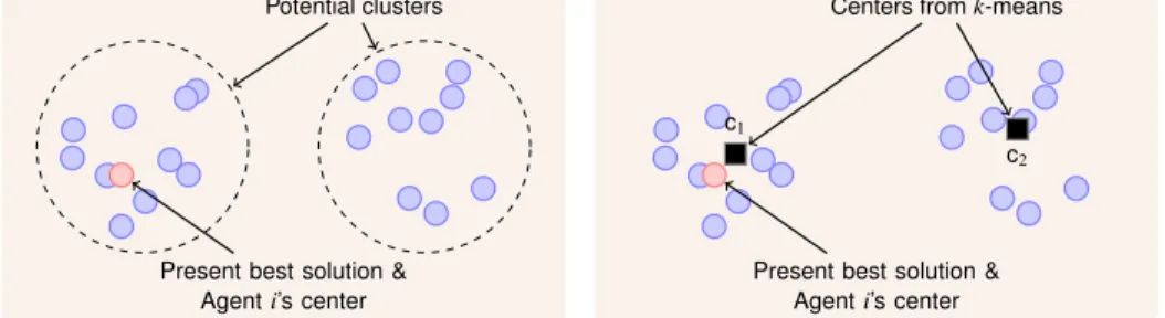
It is desirable to create an agent if it is found that points are clustered in two separate areas of a single agent’s
sub-region, as illustrated in Fig.4(a). Such a situation can occur if there are two optima in a subregion.
Potential clusters
Present best solution & Agenti’s center
(a) Potential clusters within a sub-region
Centers fromk-means
Present best solution & Agenti’s center c1
c2
(b) Clusters from k-means New agentj’s center
Present best solution & Agenti’s center
c2
(c) Final clusters after moving centers to present best solution and nearest data point
Figure 4. Illustration of process used to create an agent j given points in a single agent i’s sub-region.
Agents are created by using k-means clustering24for two clusters (k = 2) given the points in the sub-region, where
the initial guesses of the centers are the present best solution (the current center) and the mean of the dataset. Since
k-means clustering gives centers that are not current data points as illustrated in Fig.4(b), we move the centers to
available data points to avoid more calls to evaluate the expensive functions. This is done by first measuring the distance of the centers from k-means to the present best solution, and moving the closest center to the present best solution, as we want to preserve this solution. For the other center, we measure the distance of the current data points
to the other center, and make the closest data point the other center. The final clustering is illustrated in Fig.4(c). The
result is a new agent with a center at an already existing data point, where the creating agent retains its center at its present best solution.
This final clustering is validated using the mean silhouette value of the points in the sub-region. The silhouette,
introduced by Rousseeuw,25is used to validate the number of clusters, by providing a measure of the within-cluster
tightness and separation from other clusters for each data point i for a set of points. The silhouette value for each point is given as
s(i) = b(i)− a(i)
max{a(i), b(i)} (4)
where aiis the average distance between point i and all other points in the cluster to which point i belongs, and biis
the minimum of the average distances between point i and the points in the other clusters. The values of sirange from
-1 to 1. For sinear zero, the point could be assigned to another cluster. If siis near -1, the point is misclassified, and,
characterize a clustering. In this paper, we accept the clustering if all siare greater than 0 and the average value of the
silhouette is greater than some value. 3. Create New Agents
The agents may reach a point where there is no improvement made by the overall system in several iterations (i.e., the centers of all agents have remained at the same points). For example, this can occur when each agent has located the best point in its sub-region, the area around each best point is populated by points, each agent is driven to explore for several iterations, and no other potential local optima are located. This can also occur at early iterations in which the surrogates are not well-trained in the sub-region. In order to improve exploration, a new agent is created in the design space when there is no improvement for n iterations (i.e., the centers of the sub-regions have not moved for n iterations). We call this parameter the stagnation threshold. To create a new agent, a new center is created at an already existing data point that maximizes the minimum distance from the already existing centers, thus forming a new agent. The design space is then repartitioned.
VI.
Six-Dimensional Analytical Example
In this section, we examine the six-dimensional Hartman function (Hartman 6) that is often used to test global optimization algorithms. minimize x fhart(x) =− q X i=1 aiexp − m X j=1 bi j(xj− di j)2 subject to 0≤ xj≤ 1, j = 1, 2, . . . , m = 6 (5)
In this instance of Hartman 6, q = 4 and a =h1.0 1.2 3.0 3.2iwhere
B = 10.0 3.0 17.0 3.5 1.7 8.0 0.05 10.0 17.0 0.1 8.0 14.0 3.0 3.5 1.7 10.0 17.0 8.0 17.0 8.0 0.05 10.0 1.0 14.0 D = 0.1312 0.1696 0.5569 0.0124 0.8283 0.5886 0.2329 0.4135 0.8307 0.3736 0.1004 0.9991 0.2348 0.1451 0.3522 0.2883 0.3047 0.3047 0.4047 0.8828 0.8732 0.5743 0.1091 0.0381
As we wish to locate multiple optima, we modified Hartman 6 to contain 4 distinct local optima by “drilling” two additional Gaussian holes at two locations to form two local optima, in addition to the global optimum and one local
optimum provided in the literature.26 The modified Hartman 6 function is
f(x) = fhart(x)− 0.52φ1(x)− 0.18φ2(x) (6)
where the mean and standard deviation associated with φ1 and µ1 =
h
0.66 0.07 0.27 0.95 0.48 0.13iand σ = 0.3 (all
directions), respectively. The mean and standard deviation associated with φ2and µ2 =
h
0.87 0.52 0.91 0.04 0.95 0.55i
and σ2 =0.25 (all directions), respectively. The optima are displayed in Table1. To obtain an approximate measure
of the size of the basins of attraction that contain the optima, we measured the percentage of local optimization runs that converged to each optimum. To do this, twenty-thousand points were sampled using Latin Hypercube sampling and a local optimization was performed starting at each one of these points using a SQP algorithm.
The percentage of starts that converged to an optimum is also a measure of the volume of its basin of attraction in comparison to other basins. Since Local 2 has the smallest percentage of runs, it was expected that it would be the
most difficult optimum to locate by the agents. Note, however, that in six-dimensional space a ratio of 50%9% in volume
would be produced by a ratio of 0.75 in characteristic dimension.
A. Experimental Setup
Since there are no nonlinear constraints, only the objective function is approximated by surrogates.. The three possible
Table 1. Modified Hartman6 optima and the percentage of runs that found each optimum with multiple starts and a SQP optimizer
Optimum f x percentage of runs
Global -3.33 h0.20 0.15 0.48 0.28 0.31 0.66i 50 Local 1 -3.21 h0.40 0.88 0.79 0.57 0.16 0.04i 21 Local 2 -3.00 h0.87 0.52 0.91 0.04 0.95 0.55i 9 Local 3 -2.90 h0.64 0.07 0.27 0.95 0.48 0.13i 20
agent chose the best surrogate based on PRES SRMS. The set of surrogates and the minimum number of points used
to fit each surrogate are provided in Table2. If the minimum number of points are not available, points are borrowed
from neighboring sub-regions in the order of increasing distance to the agent center, and, if the requirement is still not met, then all available points are used.
Table 2. Surrogates considered in this study
ID Description minimum # of pts for fit
1 Kriging (quadratic trend)
1.5 * # coefficients for quadratic response surface 2 Kriging (linear trend)
3 Kriging (constant trend)
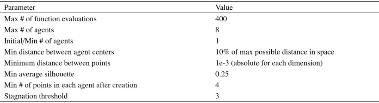
The parameters in Table3were used for all results. These parameters include maximum number of agents (e.g.,
the maximum number of computing nodes available), parameters that dictate how close points and centers can be, and parameters that define if a new agent should be created. Since we are simulating expensive function evaluations, we also fixed a computational budget to 400 function evaluations. Beyond this number, the system stops: this is our only termination criterion. Finally, we start the multi-agent system with a single agent able to split and merge with time.
Table 3. Multi-Agent Parameters for modified Hartman 6
Parameter Value
Max # of function evaluations 400
Max # of agents 8
Initial/Min # of agents 1
Min distance between agent centers 10% of max possible distance in space Minimum distance between points 1e-3 (absolute for each dimension)
Min average silhouette 0.25
Min # of points in each agent after creation 4
Stagnation threshold 3
The success and efficiency of the multi-agent approach is compared to a single agent system which performs a
classical surrogate-based optimization procedure as described in Algorithm1. However, this single agent is unable to
perform dynamic partitioning and optimizes over the whole space. This single agent has also a computation budget of 400 calls to the expensive function. The single agent configuration is a standard to which we compare our multi-agent optimizer.
In each case, (multi- or single agent), as to evaluate the capability of the algorithms to explore the search space,
we also ran several experiments for different initial DOE sizes (35a, 56, and 100) that still account for the number of
function evaluations. Therefore, for a larger initial DOE, the system executes fewer steps. For each of the cases that were studied, the results shown are the median of 50 repetitions (i.e, 50 different initial DOEs). The local optimization
problems were solved with a sequential quadratic programming (SQP) algorithm.27 DOEs are obtained using Latin
Hypercube sampling and the maximin criterion for five iterations.
aThis does not satisfy the minimum required number of points for the fit, so all points are used (a single surrogate spans the entire design space)
B. Successes to locate optima
For 50 repetitions, the success in locating a solution within some distance from the optimum with a single agent and a
multi-agent system is shown in Fig.5. This distance is the Euclidean distance normalized by the maximum possible
distance between points in the design space (here, √6). It was observed that the single agent had fewer successes
compared to the multi-agent case. In both the single and multi-agent cases, Local 2 was the optimum that was the most difficult to locate with less than 10 successes with a single agent and 32 successes with a multi-agent system. Based on the small percentage of runs that located Local 2 with multiple starts and the true function values with the
SQP optimizer (c.f. Table1), this was not unexpected.
0.02 0.04 0.06 0.08 0.1 0 10 20 30 40 50 Distance Number of successes Global 0.02 0.04 0.06 0.08 0.1 0 10 20 30 40 50 Distance Number of successes Local 1 35 56 100 0.02 0.04 0.06 0.08 0.1 0 10 20 30 40 50 Distance Number of successes Local 2 0.02 0.04 0.06 0.08 0.1 0 10 20 30 40 50 Distance Number of successes Local 3
(a) Single Agent
0.02 0.04 0.06 0.08 0.1 0 10 20 30 40 50 Distance Number of successes Global 0.02 0.04 0.06 0.08 0.1 0 10 20 30 40 50 Distance Number of successes Local 1 35 56 100 0.02 0.04 0.06 0.08 0.1 0 10 20 30 40 50 Distance Number of successes Local 2 0.02 0.04 0.06 0.08 0.1 0 10 20 30 40 50 Distance Number of successes Local 3 (b) Multi-Agent
Figure 5. For the modified Hartman 6 example, number of successes in locating each optimum with(a)a single agent and(b)multiple agents.
C. Agent Efficiency and Dynamics
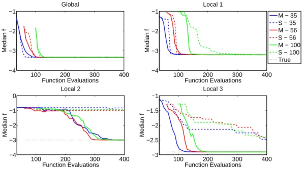
The median objective function value of the solution closest to each optimum is shown in Fig.6. For the global
optimum and Local 1, it was observed that the efficiency is nearly equal in the single and multi-agent cases. It was also observed that the smaller DOEs required fewer function evaluations to find these optima. For Local 2 and Local
100 200 300 400 −4 −3 −2 −1 Function Evaluations Median f Global 100 200 300 400 −4 −3 −2 −1 Function Evaluations Median f Local 1 M − 35 S − 35 M − 56 S − 56 M − 100 S − 100 True 100 200 300 400 −4 −3 −2 −1 0 Function Evaluations Median f Local 2 100 200 300 400 −3 −2.5 −2 −1.5 −1 Function Evaluations Median f Local 3
Figure 6. Median objective function value of solution closest to each optimum with number of function evaluations. The single agent case is denoted by “S” and the multi-agent case by “M”, with the initial DOE size represented by the number.
3, the multi-agent system has a clear advantage in finding solutions with the objective function near the true optimum value. While it is clear for the global optimum and Local 1 that smaller DOEs are more efficient, there is no clear relationship between DOE size and efficiency (consider Local 2). Recall that Local 2 was expected to be the most difficult optimum to find judging by the small percentage of runs of multiple starts with the SQP optimizer that were successful. These results confirm that exploration is required to locate Local 2, and the multi-agent system, in which exploration is an inherent feature, is more capable of finding this optimum.
Exploration by the multi-agent system was measured by the percentage of calls to the true objective function in
which exploitation or exploration occurred as shown in Fig.7. We define an exploitation call as when the agent adds
a point that minimizes the objective function. Note that we constrained the minimum distance a new point should be from an already existing data point so that multiple local optima could be located. Exploration is when a random point is added by an agent. Exploration generally occurs when exploitation has failed, meaning all starts in the sub-region resulted in points that were not far enough from existing data points or were outside of the sub-region.
We observed that the multi-agent case mostly performed exploitation with a few explorations, whereas the single agent performed exploration only 1% of the time. This could be due to the single agent seeking to tune around the global optimum and Local 1, which it locates with the fewest function evaluations. The number of times in which the an agent puts point to tune around the optimum can be reduced by increasing the minimum distance between points. In addition, it was observed that the single agent was slowly adding exploitation points in the vicinity of Local 3 as
shown in Fig.6.
Figure 8shows the median number of agents. While up to 8 agents could be created, it was observed that the
median number of agents stabilized around 4, the number of local optima. This is because once all the local optima are located, new agents are created but are soon deleted as they converge to the basins of attraction of the already found optima. 0 10 20 30 40 50 60 70 80 90 100 1 1.5 2 2.5 3 3.5 4 4.5 5 Iteration
Median Number of Agents
35 56 100
Figure 8. For a multi-agent system, the median number of agents
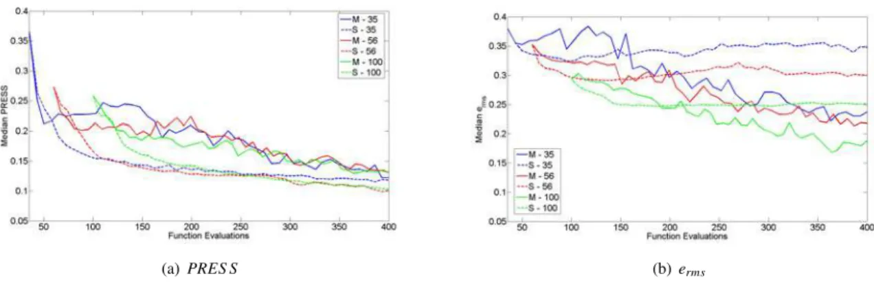
The accuracy of the surrogates was measured by the partial PRES SRMS and the error at 1000 test points by
the erms. PRES SRMS is a leave-one-out cross-validation error. In the single agent case the calculation of PRESS
is straightforward, but for the multi-agent case it is taken by calculating PRES SRMS in each sub-region and taking
the mean of the values. The values of PRES SRMS and eRMS are displayed in Fig.9. The PRES SRMS indicated
that the error was decreasing for both the single and multi-agent cases, with the single agent case slightly more
accurate. However, the eRMS provided a more global indication of the accuracy of the surrogate and showed that the
approximation made by the multiple agents improved with function evaluations more than the approximation of the single agent did. This is due to the single agent putting many points near the global optimum and Local 1, making the surrogate accurate in these locations but less accurate globally. The slow location of Local 3 by the single agent can also be partially explained by the poor accuracy of the single agent’s surrogate.
(a) PRES S (b) erms
VII.
Engineering Example: Integrated Thermal Protection System
In this section, we illustrate the multi-agent method and the importance of locating multiple candidate designs on
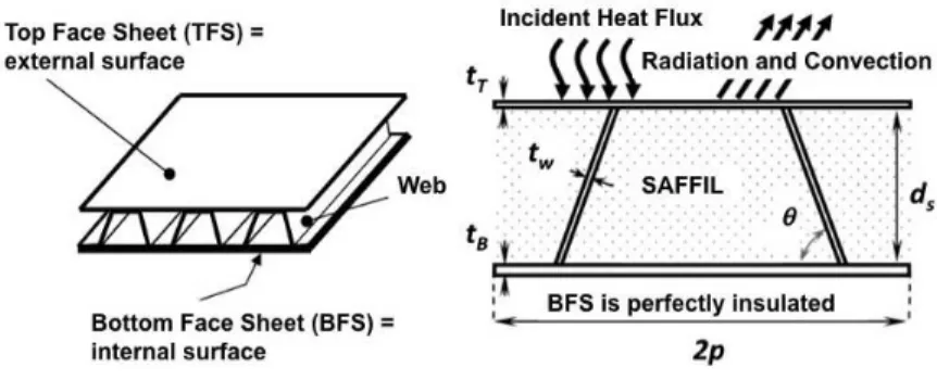
an integrated thermal protection system (ITPS). Figure10shows the ITPS panel that is studied, which is a corrugated
core sandwich panel concept. The design consists of a top face sheet and webs made of titanium alloy (Ti-6Al-4V), and
a bottom face sheet made of beryllium. Saffil R
foam is used as insulation between the webs. The relevant geometric
variables of the ITPS design are also shown on the unit cell in Figure10. These variables are the top face thickness
(tT), bottom face thickness (tB), thickness of the insulation foam (dS), web thickness (tw), and corrugation angle (θ).
The mass per unit area is calculated using Eq.(7)
Figure 10. Corrugated core sandwich panel ITPS concept
f = ρTtT+ ρBtB+
ρwtwdS
psin θ (7)
where ρT, ρB, and ρware the densities of the materials that make up the top face sheet, bottom face sheet, and web,
respectively.
The optimization problem to minimize the mass subject to constraints on the maximum bottom face sheet
temper-ature TBand maximum stress in the web σwis shown in Eq.(8).
minimize
x={tw,tB,dS,tT,θ} f(x)
subject to TB(x)− TBallow≤ 0
σw(x)− σalloww ≤ 0
xL,i≤ xi≤ xU,ifor i = 1 . . . 5
where xL= h 1.31 6.00 60.6 1.13 75.3i and xU= h 1.96 9.00 60.6 1.27 84.8i (8)
The bottom face sheet temperature and the maximum stress, which are both functions of the design variables all five
design variables, are constrained to by their maximum allowable values. As described in Sec.II, the 3-D problem,
where the bottom face, web, and foam thicknesses were the design variables, had three distinct feasible regions con-taining three local optima. For the 5-D problem, we found the true optima by solving the true optimization problem
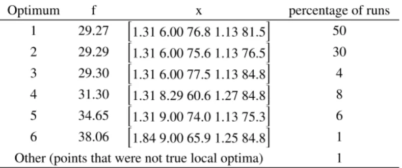
with 1000 random initial points with the SQP optimizer. Table4lists the optima that were found and gives the
per-centage of the runs that located each optimum. As the perper-centage of runs that converge to each optimum is a measure of the difficulty to locate the optimum, we observed that optimum 3 would be the most difficult to locate by the agents.
A. Experimental Setup
In this example, we follow the same experimental setup as for the modified Hartman6 example, with the parameters
provided in Table3. However, the computational budget is fixed at 120 evaluations of the expensive functions and the
maximum number of agents is raised to 10. As the objective function, the mass, calculated by the simple expression
in Eq.(7) the agents only approximate the two limit states g1and g2with surrogates. The initial DOE size was varied
Table 4. 5-D ITPS example optima and the percentage of runs that found each optimum with multiple starts and a SQP optimizer
Optimum f x percentage of runs
1 29.27 h1.31 6.00 76.8 1.13 81.5i 50 2 29.29 h1.31 6.00 75.6 1.13 76.5i 30 3 29.30 h1.31 6.00 77.5 1.13 84.8i 4 4 31.30 h1.31 8.29 60.6 1.27 84.8i 8 5 34.65 h1.31 9.00 74.0 1.13 75.3i 6 6 38.06 h1.84 9.00 65.9 1.25 84.8i 1 Other (points that were not true local optima) 1
B. Successes to locate optima
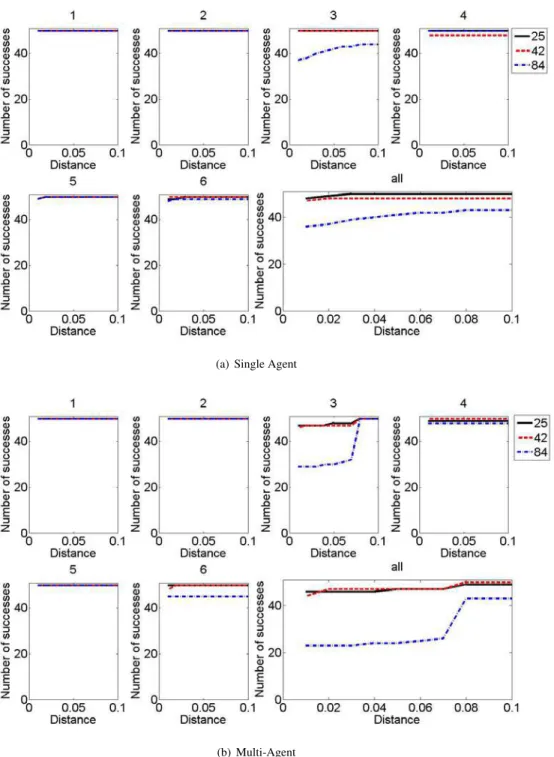
For 50 repetitions, the number of successes in locating a feasible solution within some distance from each optimum
is provided in Fig.11. The differences in the number of successes between the single and multi-agent cases for all
optima were small, with the exception of optimum 3. It was observed that the multi-agent system was less successful at locating optimum 3, particularly with the initial DOE size of 84. In comparing the success of locating all optima in a single repetition, it was clear that the success in locating all optima was dictated by the success in locating optimum 3.
(a) Single Agent
(b) Multi-Agent
Figure 11. For the 5-D ITPS example, the number of successes in locating a feasible solution within some distance from each optimum by a(a)single agent and(b)multiple agents.
C. Agents Efficiency and Dynamics
The median objective function value of the closest solution to each optimum is shown in Fig.12. It should be noted that
all solutions were feasible and that in all cases the smallest initial DOE size of 25 was the most efficient. For optima 1, 2, and 4, it was observed that the differences between the single and multi-agent cases with varying initial DOEs were small. Within 30 function evaluations, both the single and multi-agent cases were able to locate each optimum. For optima 5 and 6, it is clear that the single agent is more efficient that the multi-agent, locating the optimum with 5-10 fewer function evaluations. For optimum 3, which both agents had difficulty locating, we observed that the single agent is clearly much more efficient than the multiple agents. Note that for all initial DOE sizes, the closest solution to optimum 3 is at optimum 1 ( f = 29.27), which is not unexpected as the two optima are only a distance of 0.16 (in
the normalized design space and normalized by √5) apart making these the closest pair of all the optima.
(a) Opt 1 (b) Opt 2
(c) Opt 3 (d) Opt 4
(e) Opt 5 (f) Opt 6
Figure 12. For the 5-D ITPS example, the median f of the solution nearest to each optimum. The single agent case is denoted by “S” and the multi-agent case by “M”, with the initial DOE size represented by the number.
Figure13displays the median number of agents. Though up to 10 agents could be created, the median number of
agents stabilized around 3. Figure14compares the number of exploitations and explorations for the single and
multi-agent cases for different initial DOE sizes. We observed that, although the number of multi-agents stabilizes at 3, exploitation is still performed more by the multiple agents considering the constraint on the minimum distance between points. In all multi-agent cases, there was more exploitation than exploration. For the single agent, there was more exploration, except for the initial DOE of 84 points. This was due to the ability of the single agent to locate the multiple optima quickly with exploitation iterations due the constraint on the minimum distance between points. After this occurred, the single agent performed more exploration, which aided in the location of the most difficult optimum to locate, optimum 3. For the initial DOE of 84, the single agent had fewer evaluations in which to locate all optima, so exploitation was dominant.
(a) Number of active agents (b) Number of iterations vs function evaluations Figure 13. For the 5-D ITPS example, the number of active agents and the number of iterations.
The superior performance by the single agent was also attributed to the accuracy of its surrogate approximations.
Fig.15compares the PRES SRMS of each surrogate for the single and multi-agent cases. The PRES SRMS decreased
with increasing number of function evaluations after it initially increased. This was due to the placement of points around the optima, which made the surrogate less accurate further from the optima. This led to large errors when a point that was far away from other points was left out in calculating the cross-validation error. As more exploration
points were added, the PRES SRMS was reduced. For the multi-agent case, we observed that the PRES SRMS increased
through the function evaluations. This was due to the large number of points put around the optima in exploitation iterations, which outnumbered the exploration iterations.
Figure 15. Median PRES SRMSof the surrogates of the limit states for the 5-D ITPS example
Figure16displays the error at 1000 test points eRMS. We observed much of the same trends as with PRES SRMS,
with the surrogates in the multi-agent case decreasing in accuracy while the surrogates of the single agent cases increased accuracy.
VIII.
Discussion
The single agent approach showed a clear advantage over the multi-agent method in the ITPS example in Sec.VII.
The single agent approach is simple : a global surrogate is used and a constraint on the minimum distance between points is the only way to instigate exploration of the design space. It is advantageous in its simplicity and ease of implementation, but its success depends on how well a single surrogate can approximate the global behavior. The
accuracy measures of the limit states for the ITPS example in Fig.16show that the global surrogate is indeed more
accurate than several local surrogates. Upon further investigation of the temperature and stress trends in the design space, it was found that simple quadratic response surfaces over the design space were sufficient approximations.
On the contrary, the modified Hartman 6 function presented in Sec.VI, for which the unmodified version is often
used as a benchmark function for surrogate-based global optimization algorithms, is thought to be more complex
compared to the ITPS example. The error at test points (c.f. Fig.9(b)) shows that the accuracy of the local surrogates
is slightly better than that of the single agent’s global surrogate. In this example, we observed that the multi-agent method can be successful and efficient.
What does this say about this multi-agent algorithm? Based on these two examples, the success rate and efficiency of the multi-agent method may be dependent on having higher accuracy local surrogates compared to a global surro-gate. Otherwise, simpler algorithms may be more efficient. Further investigation on the need for local surrogates is required, and a study that uses a global surrogate with the agent-based dynamic design space partitioning is planned. It will allow us to study separately two ingredients that make up the method investigated here: local versus global surrogate and space partitioning to increase chances of visiting many basins of attraction leading to different local optima.
IX.
Conclusions and Future Work
This paper introduced a multi-agent methodology for optimization that dynamically partitions the design space as to find multiple optima. Multiple designs provide insurance against discovering that late in the design process a design is poor due to modeling errors or overlooked objectives or constraints. The method used surrogates to approximate expensive functions and agents optimized using the surrogates in the regions. The centers of the agents’ sub-regions moved to stabilize around optima, and agents were created and deleted at run-time as a means of exploration and efficiency, respectively.
The method was applied to two examples, an analytical test function and a practical engineering example. It was observed that for problems in which the behavior is simple to approximate with a global surrogate, the simpler single agent is more efficient and successful than the multiple agents. For the more complicated test function, in which local surrogates were slightly more accurate, the multiple agents outperformed the single agent. These results lead us to believe that the success of the current agent algorithm is dependent on local surrogates being more accurate than a global surrogate.
For future work, we plan to focus on using a global surrogate with the dynamic partitioning still in place. The reason for this is two-fold: (i) in the authors’ experience, there are few situations in which local surrogates are signif-icantly more accurate than a global surrogate, (ii) the complication of managing points between sub-regions to create
surrogates is removed. Efficient Global Optimization28 (EGO) is a popular global optimization algorithm that uses
a global surrogate and adds points based on the present best solution (the present best data point). It is planned to modify the EGO algorithm for use with the dynamic design space partitioning, in which each sub-region has its own present best solution.
The proposed agent optimization method also has a great potential for parallel computing. As the number of computing nodes n increases, the calculation of the expensive objective and constraints functions scales with 1/n in terms of wall-clock time. But the speed at which problems can be solved then becomes limited by the time taken by the optimizer, i.e., the process of generating a new candidate solution. In the algorithm we have developed, the optimization task itself can be divided among the n nodes through agents. We plan to explore how agents can provide a useful paradigm for optimizing in parallel, distributed, asynchronous computing environments.
Acknowledgments
This work has benefited from funding from Agence Nationale de la Recherche (French National Research Agency) with ANR-09-COSI-005 reference. This work was also supported by NASA under award No.NNX08AB40A and the Air Force Office of Scientific Research under award FA9550-11-1-0066. Any opinions, findings, and conclusions or
recommendations expressed in this material are those of the author(s) and do not necessarily reflect the views of the ANR, NASA, or the AFOSR.
References
1Jin, R., Du, X., and Chen, W., “The use of metamodeling techniques for optimization under uncertainty,” Structural and Multidisciplinary
Optimization, Vol. 25, No. 2, 2003, pp. 99–116.
2Queipo, N. V., Haftka, R. T., Shyy, W., and Goel, T., “Surrogate-based analysis and optimization,” Progress in Aerospace Sciences, Vol. 41,
2005, pp. 1–28.
3Sacks, J., Welch, W. J., J., M. T., and Wynn, H. P., “Design and analysis of computer experiments,” Statistical Science, Vol. 4, No. 4, 1989,
pp. 409–435.
4Simpson, T. W., Peplinski, J. D., Koch, P. N., and Allen, J. K., “Metamodels for computer based engineering design: survey and
recommen-dations,” Engineering with Computers, Vol. 17, No. 2, 2001, pp. 129–150.
5Zhao, D. and Xue, D., “A multi-surrogate approximation method for metamodeling,” Engineering with Computers, Vol. 27, 2005, pp. 139–
153.
6Wang, G. G. and Simpson, T. W., “Fuzzy Clustering Based Hierarchical Metamodeling for Design Space Reduction and Optimization,”
Engineering Optimization, Vol. 36, No. 3, 2004, pp. 313–335.
7Voutchkov, I. and Keane, A. J., “Multiobjective optimization using surrogates,” 7th International Conference on Adaptive Computing in
Design and Manufacture, Bristol, UK, 2006, pp. 167–175.
8Samad, A., Kim, K., Goel, T., Haftka, R. T., and Shyy, W., “Multiple surrogate modeling for axial compressor blade shape optimization,”
Journal of Propulsion and Power, Vol. 25, No. 2, 2008, pp. 302–310.
9Viana, F. A. C. and Haftka, R. T., “Using multiple surrogates for metamodeling,” 7th ASMO-UK/ISSMO International Conference on
Engi-neering Design Optimization, 2008.
10Glaz, B., Goel, T., Liu, L., Friedmann, P., and Haftka, R. T., “Multiple-surrogate approach to helicopter rotor blade vibration reduction,”
AIAA Journal, Vol. 47, No. 1, 2009, pp. 271–282.
11Shoham, Y. and Leyton-Brown, K., Multiagent Systems: Algorithmic, Game-Theoric, and Logical Foundations, Cambridge University Press,
2009.
12Modi, P. J., Shen, W., Tambe, M., and Yokoo, M., “ADOPT: Asynchronous Distributed Constraint Optimization with Quality Guarantees,”
Artificial Intelligence, Vol. 161, No. 2, 2005, pp. 149–180.
13Holmgren, J., Persson, J. A., and Davidsson, P., “Agent Based Decomposition of Optimization Problems,” First International Workshop on
Optimization in Multi-Agent Systems, 2008.
14Beasley, D., Bull, D. R., and Martin, R. R., “A sequential niche technique for multimodal function optimization,” Evolutionary computation,
Vol. 1, No. 2, 1993, pp. 101–125.
15Hocaoglu, C. and Sanderson, A. C., “Multimodal function optimization using minimal representation size clustering and its application to
planning multipaths,” Evolutionary Computation, Vol. 5, No. 1, 1997, pp. 81–104.
16Brits, R., Engelbrecht, A. P., and van den Bergh, F., “Locating multiple optima using particle swarm optimization,” Applied Mathematics
and Computation, Vol. 189, No. 2, 2007, pp. 1859–1883.
17Parsopoulos, K. E. and Vrahatis, M. N., Artificial Neural Networks and Genetic Algorithms, chap. Modification ofthe Particle Swarm
Optimizer for Locating All the Global Minima, Springer, 2001, pp. 324–327.
18Li, X., “Adaptively Choosing Neighbourhood Bests Using Species in a Particle Swarm Optimizer for Multimodal Function Optimization,”
Genetic and Evolutionary Computation (GECCO 2004), Vol. 3102 of Lecture Notes in Computer Science, 2004, pp. 105–116.
19Nagendra, S., Jestin, D., Gurdal, Z., Haftka, R. T., and Watson, L. T., “Improved genetic algorithm for the design of stiffened composite
panels,” Computers & Structures, Vol. 58, No. 3, 1996, pp. 543–555.
20Li, J. P., Balazas, M. E., Parks, G., and Clarkson, P. J., “A Species Conserving Genetic Algorithm for Multimodal Function Optimization,”
Evolutionary Computation, Vol. 10, No. 3, 2002, pp. 207–234.
21Torn, A. and Zilinskas, A., “Global Optimization,” Lecture Notes in Computer Science 350, Springer Verlag, 1989. 22Kleijen, J., Design and analysis of simulation experiments, Springer, 2008.
23Aurenhammer, F., “Voronoi diagrams: a survey of a fundamental geometric data structure,” ACM Computing Surveys (CSUR), Vol. 23, No. 3,
1991, pp. 345–405.
24Hartigan, J. and Wong, M., “Algorithm AS 136: A K-Means Clustering Algorithm,” Journal of the Royal Statistical Society. Series C
(Applied Statistics), Vol. 28, No. 1, 1979, pp. 100–108.
25Rousseeuw, P. J., “Silhouettes: a Graphical Aid to the Interpretation and Validation of Cluster Analysis,” Computational and Applied
Mathematics, Vol. 20, 1987, pp. 53–65.
26Viana, F. A. C., Multiple Surrogates for Prediction and Optimization, Ph.D. thesis, University of Florida, 2011. 27MATLAB, version 7.9.0.529 (R2009b), chap. fmincon, The MathWorks Inc., Natick, Massachusetts, 2009.
28Jones, D. R., Schonlau, M., and Welch, W. J., “Efficient Global Optimization of Expensive Black-Box Functions,” Journal of Global