HAL Id: hal-00633223
https://hal.archives-ouvertes.fr/hal-00633223
Submitted on 18 Oct 2011
HAL is a multi-disciplinary open access
archive for the deposit and dissemination of
sci-entific research documents, whether they are
pub-lished or not. The documents may come from
teaching and research institutions in France or
abroad, or from public or private research centers.
L’archive ouverte pluridisciplinaire HAL, est
destinée au dépôt et à la diffusion de documents
scientifiques de niveau recherche, publiés ou non,
émanant des établissements d’enseignement et de
recherche français ou étrangers, des laboratoires
publics ou privés.
Solving the Resource Allocation Problem in a
Multimodal Container Terminal as a Network Flow
Problem
Elisabeth Zehendner, Nabil Absi, Stéphane Dauzère-Pérès, Dominique Feillet
To cite this version:
Elisabeth Zehendner, Nabil Absi, Stéphane Dauzère-Pérès, Dominique Feillet. Solving the Resource
Allocation Problem in a Multimodal Container Terminal as a Network Flow Problem. Jürgen W. Böse,
Hao Hu, Carlos Jahn, Xiaoning Shi, Robert Stahlbock, Stefan Voß. Computational Logistics, 6971,
Springer, pp.341-353, 2011, Lecture Notes in Computer Science, Volume 6971/2011,
�10.1007/978-3-642-24264-9_25�. �hal-00633223�
Multimodal Container Terminal as a Network
Flow Problem
Elisabeth Zehendner, Nabil Absi, St´ephane Dauz`ere-P´er`es, and Dominique Feillet
Ecole des Mines de Saint-Etienne, CMP, site Georges Charpak, 13541 Gardanne, France
{zehendner,absi,dauzere-peres,feillet}@emse.fr
Abstract. Continuously increasing global container trade and pressure from a limited number of large shipping companies are enforcing the need for efficient container terminals. By using internal material handling re-sources efficiently, transfer times and operating costs are reduced. We focus our study on container terminals using straddle carriers for trans-portation and storage operations. We assume that straddle carriers are shared among maritime and inland transport modes (truck, train, barge). The problem is thus to decide how many resources to allocate to each transport mode in order to minimize vehicle (vessel, truck, train, barge) delays. We present a mixed integer linear programming model, based on a network flow representation, to solve this allocation problem. The mod-ular structure of the model enables us to represent different container terminals, transport modes and service strategies. We present parts of our model and exemplary applications for a terminal at the “Grand Port Maritime de Marseille” in France.
Keywords: container terminal, resource allocation, intermodal trans-portation, mixed integer linear programming
1
Introduction
In intermodal transportation, container terminals play the role of exchange hubs. They offer transfer facilities to move containers from vessels to trucks, trains and barges and vice versa. Due to the pressure from a limited number of large shipping companies, terminals, especially geographical close ones, face strong competition. Their competitiveness is particularly marked by vessel turnaround times. But recently, the competitiveness of a container terminal is becoming more and more a function of its delays and costs for transport to and from the hinterland. One reason is that inland transportation costs account for a large part of total costs for container shipping (40% to 80% according to [6]). Other reasons are an increased interest in door-to-door services and environmental aspects (CO2 emissions). An efficient allocation of internal material handling
have to spend at the terminal and renders the terminal more competitive. In this study, we present a mixed integer linear programming model to determine an optimal resource allocation minimizing vehicle (vessel, truck, train, barge) delays.
Numerous studies deal with different optimization problems arising at con-tainer terminals. Only a few deal with the resource allocation problem and they mostly neglect inland transport modes. [3] formulates the allocation problem of quay cranes, transport vehicles and yard cranes to vessels as a network de-sign problem. The objective is to determine the cheapest allocation to serve all vessels. [1] presents a predictive control approach based on a queuing model to allocate available resources to vessels, truck and trains. The aim is to minimize the turnaround time of vehicles. [5] presents, among other, a Markovian decision model to determine optimal policies for fleet management in real time, minimiz-ing fleet operatminimiz-ing costs and vessel waitminimiz-ing costs. [7] determines the number of vehicles required to transport containers between the quay and the yard by a disjoint paths problem. Other studies aim at minimizing truck delays but con-sider scheduling rather than allocation problems. [4] develops a general model to assign jobs to container terminal resources and to temporally arrange jobs with precedence constraints and sequence-dependent setup times. [2] develops an assignment algorithm that dynamically matches straddle carriers to waiting trucks. The aim is to minimize truck serving times and empty travels of straddle carriers.
In this paper, we propose a mixed integer linear program to allocate internal material handling resources (straddle carriers) to different vehicles arriving at a terminal. Our objective is to minimize vehicle delays with focus on landside transport modes (trucks, trains, barges). Section 2 presents the resource alloca-tion problem at a terminal. In Secalloca-tion 3, a basic resource allocaalloca-tion problem is formulated as a network flow model. Possible service strategies applied to serve different vehicles are indicated in Section 4. The basic network flow model may be adapted to these service strategies. We present an exemplary extension of the core model to represent a terminal at the “Grand Port Maritime de Mar-seille” in Section 5. In Section 6, we show and discuss experiments of the model to determine a resource allocation minimizing vehicle delays and to determine the number of resources needed to cope with the expected demand. Section 7 concludes the paper.
2
The Resource Allocation Problem
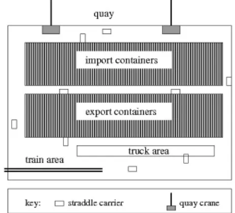
A container terminal has to provide transfer facilities for two types of container flows: Import and export containers. Import containers arrive on vessels, are un-loaded, stored at the yard, and finally transferred to landside gates where they are loaded on trucks, trains or barges. Export containers pass the terminal in the opposite direction. We concentrate our study on terminals using manned Strad-dle Carriers (called SC in the sequel) for transportation (between the quay, the yard and landside transfer points) and storage operations. Figure 1 illustrates
Fig. 1. Schematic View of a Container Terminal
the layout of such a container terminal. It presents the different areas of the terminal. Vessels and barges are loaded/unloaded at the quay by quay cranes. Trucks and trains are loaded/unloaded in specific areas. Containers are tem-porarily stored at the yard. In most cases, import and export containers are stored separately in dedicated areas. Straddle carriers move containers within the terminal.
Normally, dockers driving SCs are hired on short-term (e.g., the day before). This allows terminal operators to adapt their capacity from day to day via the number of hired dockers. For organizational reasons, manned straddle carriers are assigned to one type of tasks (e.g., serve trucks or serve a vessel) for a certain period. The arising allocation problems are to determine the needed capacity for a given day and to allocate available SCs to different vehicles arriving over the day. We focus our study on the landside part of the terminal. Our aim is to minimize the time the vehicles of the different landside transport modes stay at the terminal. We assume that arrival times and due dates (i.e. departure times) for vessels are given (e.g., imposed by the carrier or determined by the terminal operator) and that each vessel has to be served within its time window. Hence, no delays are allowed for vessels. However, our model can be extended to also minimize potential delays of vessels.
3
Core Network Flow Model
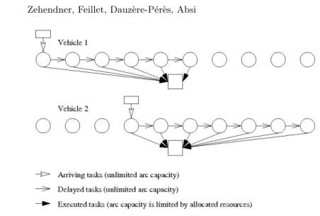
We model the resource allocation problem as a network flow problem, where containers to be moved are flows in the network and arc capacities are limited by the number of allocated resources. Our model is inspired by the approach pre-sented in [3]. Before stating the actual implementation as a mixed integer linear program, we explain the underlying idea with the help of Figure 2, which repre-sents a terminal with two vehicles arriving over the day. One network flow model is implemented for each vehicle. The round nodes stand for the discrete time pe-riods of the working day (1-10). The rectangular nodes, which are sources of
Fig. 2. Resource Allocation Problem as a Network Flow Model
flow, represent the arrival of vehicles with their associated demand for container movement requests. Each source is connected to the period corresponding to the arrival of the vehicle. The square nodes represent sinks of flow. The flows from a period node to a sink represent the number of container movements executed per period and per vehicle. Capacities on these arcs represent the maximum number of container movements that may be executed per period and per vehicle. These capacities are proportional to the number of resources allocated to the vehicle in the corresponding period. The total number of allocated resources cannot ex-ceed the total number of available resources at the terminal. The flows between two periods represent unexecuted tasks which are transferred to the next period. These arcs exist only if it is permitted to delay tasks. Note that an independent submodel is implemented for each vehicle and that those submodels are only related by one constraint limiting the total number of allocated resources. This modular structure makes it possible to include vehicle specific constraints to each submodel.
We now state the mixed integer linear program formulating these network flows. For our resource allocation problem, the situation at a container terminal may be represented by the expected workload and the terminal’s capacity. The expected workload is determined by the number of vehicles with their arrival times, their due dates and their number of required container movement requests. The terminal’s capacity is given by the number of available SCs and the average number of containers a SC can handle per period. We assume that resources may be reallocated only at discrete points in time and that all tasks have to be executed at the end of the time horizon (e.g., end of the working day).
Our objective is to provide the terminal operator with a tool to estimate the number of SCs needed to handle with the expected workload and to pro-pose a possible allocation of these resources to different vehicles. The detailed
scheduling and routing of SCs is not addressed in this study. We assume that the Terminal Operating System (TOS) uses the rough allocation of our model to determine a detailed schedule. Therefore, we use average values on the num-ber of tasks a resource can handle per shift rather than real travel times. The model is used for the resource allocation problem for the following day. There-fore, information about vehicles arrival and departure times and the number of containers to be moved are quite reliable. This allows considering information related to vehicles as deterministic. Major disruptions, however, can be handled by recomputing the model since this takes only seconds. In addition, we took into account that a container terminal is a highly dynamic and uncertain work environment. We analyzed the quality of the resource allocation obtained by the optimization model in a stochastic environment via a discrete event simulation. Results confirmed that the proposed resource allocation performs well. Details on the simulation model and the validation process are presented in [8].
We use the following sets, parameters and variables to describe the expected workload, the terminal’s capacity and the container flows in the network.
Sets and parameters:
T Number of time periods describing the time horizon M Number of transport modes being served at the terminal
Im Number of vehicles of transport mode m arriving during the time horizon
T Set of all time periods, T = {1, . . . , T } M Set of all transport modes, M = {1, . . . , M }
Im Set of all vehicles of transport mode m, Im= {1, . . . , Im}
st Number of available resources in period t
˜
dmi Period t in which vehicle i of transport mode m has to be ready for departure
rim Period t in which vehicle i of transport mode m arrives at the terminal pmi Total number of tasks to be carried out for vehicle i of transport
mode m
hm Average number of tasks a SC serving transport mode m can handle
per period (hm≥ 1)
Variables: Xm
i,t Number of resources allocated to vehicle i of transport mode m in
period t Wm
i,t Number of tasks executed in period t for vehicle i of transport mode
m, depending on the number of allocated resources Zm
i,t Number of non-executed tasks in period t for vehicle i of transport
mode m which are transferred to period t + 1
The constraints below formulate the basic network flow model for all vehicles arriving at the terminal. This core model determines a resource allocation to serve each vehicle within its time window (if such a solution exists).
Wi,tm≤ h m · Xi,tm ∀m ∈ M, i ∈ I m , t ∈ T (1) Wi,tm≥ hm· (Xm i,t− 1) + 1 ∀m ∈ M, i ∈ I m, t ∈ T (2) Zi,tm=( p m i − W m i,t, t = r m i Zi,t−1m − Wi,tm, ∀t = r m i + 1, . . . , ˜d m i ∀m ∈ M, i ∈ Im (3) Zi, ˜mdm i = 0, ∀m ∈ M, i ∈ Im (4) M X m=1 Im X i=1 Xi,tm≤ st ∀t ∈ T (5) Wi,tm, Zi,tm∈ N+ ∀m ∈ M, i ∈ Im, t ∈ T (6) Xi,tm∈ N+ ∀m ∈ M, i ∈ Im, t ∈ T (7)
Constraint (1) defines the arc capacity limiting the flow of executed container tasks. It makes sure that the number of served tasks per vehicle and per period does not exceed the capacity of resources allocated to this vehicle. Constraint (2) imposes that each allocated resource executes at least one task and prevents allocating excess resources. This makes the solution more comprehensible. Con-straint (3) formulates the mass balance conCon-straint for arriving, executed and delayed tasks for each vehicle. It also ensures that no container movement re-quests are executed prior to a vehicle’s arrival. Constraint (4) imposes that each vehicle is completely served prior to its departure. Constraint (5) guarantees that the total number of allocated resources does not exceed the number of re-sources available at the terminal. This constraint links the otherwise independent models for each vehicle. Constraint (6) ensures that tasks are always completely executed within one period (transported from their origin to their destination) or not at all. Constraint (7) imposes that resources are allocated to exactly one vehicle per period by preventing partial allocations of resources to vehicles. If resources may be shared among different vehicles per period Constraint (7) has to be replaced by Constraint (7a) which allows a partial resource allocation to vehicles.
4
Service Strategies at Terminals
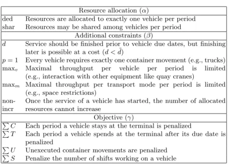
Container terminals serve different transport modes like vessels, trucks, trains and barges. These vehicles differ with regard to cargo volume, operating costs, knowledge and reliability of arrival dates, due dates and required handling equip-ment. Therefore, each transport mode is served with a specific strategy taking into account its characteristics. Service strategies for the same transport mode may also differ from terminal to terminal. We introduce a notation α|β|γ to de-scribe the service strategy for one transport mode. Table 1 presents an overview of different values that may be taken by α, β and γ. α specifies if resources may be shared among different vehicles or not. β indicates additional constraints like limits on the maximum throughput per period. γ represents the objective we want to achieve. This may be to minimize the time a vehicle spends at the ter-minal, the number of unexecuted tasks when the vehicle leaves the terminal or the number of shifts used to work on the vehicle.
Table 1. α|β|γ Notation to Describe Service Strategies Resource allocation (α)
ded Resources are allocated to exactly one vehicle per period shar Resources may be shared among vehicles per period
Additional constraints (β)
d Service should be finished prior to vehicle due dates, but finishing later is possible at a cost (d < ˜d)
p = 1 Every vehicle requires exactly one container movement (e.g., trucks) maxv Maximal throughput per vehicle per period is limited
(e.g., interaction with other equipment like quay cranes)
maxm Maximal throughput per transport mode per period is limited
(e.g., space restrictions)
non-incr
Once the service of a vehicle has started, the number of allocated resources cannot increase
Objective (γ)
P C Each period a vehicle stays at the terminal is penalized
P T Each period a vehicle spends at the terminal after its due date is penalized
P U Unexecuted container movements are penalized P S Penalize the number of shifts working on a vehicle
5
Adaptation to the Case of a Container Terminal in
Marseilles
Our core model determines a resource allocation to serve every vehicle within its time window. Thanks to the modularity of our model we can formulate trans-port mode specific submodels reflecting the specific service strategies by adding
parameters, variables and constraints. Presenting all cases is out of the scope of this paper. We rather present an exemplary adaptation to a container termi-nal at the “Grand Port Maritime de Marseille” in France. This termitermi-nal serves vessels, barges, trains and trucks. For the sake of concision, we present only the adapted submodels for barges (m=1) and trains (m=2). For trucks and vessels, we indicate only their service strategies without detailing their implementation.
5.1 Barge (m=1)
The time a barge spends at the terminal (waiting and service times) should be minimized. Resources are allocated to exactly one barge and are not shared among barges. The maximum number of resources handled per period is limited by the throughput of quay cranes. This service strategy may be represented by ded| maxv|P C with our notation. We introduce parameter qimto represent
the maximum throughput per period of the quay cranes assigned to the barge. Constraint (8) ensures that this limit is satisfied. We also introduce a binary variable, Ym
i,t, to measure the delay of a vehicle. It indicates at each period if
the vehicle is completely served and may leave the terminal (Ym
i,t = 0) or not
(Ym
i,t = 1). Each period the vehicle spends at the terminal is penalized in the
objective function. Constraints (9) and (10) together with the objective function assert that Ym
i,t is equal to zero if and only if the service of a vehicle is finished.
min Im X i=1 T X t=rm i Yi,tm for m = 1 s.t. Constraints (1)-(4), (6)-(7) for m = 1 Wi,tm≤ qim m = 1, ∀i ∈ Im, t ∈ T (8) Yi,tm≥ Z m i,t pm i m = 1, ∀i ∈ Im, t = rim, . . . , T (9) Yi,tm∈ {0; 1} (10) 5.2 Train (m=2)
Trains are served at the rail station. Railcars stay at the terminal over the day and are picked up by an engine according to a fixed schedule every day. There is a cost for each container remaining after the departure of its associated train. SCs are shared among trains. They transport containers from the common rail buffer to the yard and vice versa. The loading/unloading of trains is done by reach stackers which are not included in the model. This service strategy is equivalent
to shar|d|P U with d = ˜d. We allow resource sharing among trains, but not among different transport modes. We introduce variable ˆXtm and Constraints (4a) and (11) to limit resource sharing on vehicles of the same transport mode.
ˆ
Xtmis the total number of resources allocated to transport mode m in period t.
We also introduce variable Ui,tm to indicate the number of container movement requests remaining unexecuted at the train’s departure. Each unexecuted task is penalized in the objective function. Constraint (4) is modified to consider unexecuted tasks. min Im X i=1 Uim for m = 2 s.t.
Constraints (1)-(3), (6)-(7a) for m = 2
Zi, ˜md− Ui,tm= 0 m = 2, ∀i ∈ I m (4a) Im X i=1 Xi,tm≤ ˆXtm m = 2, ∀t ∈ T (11) ˆ Xtm∈ N+ m = 2, ∀t ∈ T (12)
5.3 Vessels and Trucks
Vessels have to be served during their imposed time windows. It is not allowed to plan a delayed departure of a vessel, but there is no incentive to finish earlier. The objective is to serve the vessel with the smallest number of shifts. SCs are allocated to exactly one vessel and are not shared among vessels. The service of a vessel requires some preparation and coordination. Therefore, no additional SCs are allocated to a vessel once its service has started, but retrieving superfluous SCs is possible. The maximum throughput per period is limited by the capacity of quay cranes. This service strategy is equivalent to ded|non-incr,maxv|P S.
Arriving trucks are assigned to parking slots where they are loaded and unloaded directly by SCs. Trucks should be served as fast as possible. We assume that each truck loads or unloads exactly one container. SCs are shared among trucks. This service strategy is equivalent to shar|p = 1|P C.1
1 To reduce the problem size we represent all trucks arriving over the working day
by one aggregated network flow model. To do so, vehicle specific parameters and variables have to be aggregated and Constraint (3) has to be modified to include arrivals in several periods.
5.4 The Entire Terminal
To represent the entire container terminal, we only have to combine the inde-pendent transport mode specific submodels. To do this, we sum the respective objective functions, include all constraints into the combined model and add one constraint limiting the number of allocated SCs. Weights cm may be added in
the objective function to represent priorities among different transport modes. To illustrate this procedure, we present the combination of the barge and the train submodels. We observe that the objective function is the sum of the delay of barges and the number of containers left at the terminal at train departures. All constraints of the two submodels are included. Constraint (5a) is added to make sure that only available resources are allocated. It takes into account the fact that resources may be shared among trains. The submodels for vessels and trucks may be added in the same manner by including their objective functions, their specific constraints and by updating Constraint (5a).
min c1· I1 X i=1 T X t=r1 i Yi,t1 + c2· I2 X i=1 Ui2 s.t. Constraints (1)-(3), (6) for m = 1, 2 Constraints (4),(7), (8)-(10) for m = 1 Constraints (4a),(7a), (11), (12) for m = 2
I1 X i=1 Xi,t1 + X 2 t ≤ st ∀t ∈ T (5a)
6
Numerical Experiments and Results
Experiments were run on actual data of one of the terminals in Marseilles. The time horizon is set to one working day and is divided into 21 one-hour periods. The data provides information on the number of vessels (0-2), of trains (1) and of barges (0-1) arriving per day. It also indicates arrival and departure times and the number of container movement requests per vehicle and the aggregated demand for trucks (280-770 requests). Information on the available SCs, the average number of resources a SC can handle per period and the chosen service strategy per transport mode were obtained via discussion with the terminal operator. The analysis was also carried out for a division of the working day into 42 half-hour periods. The analysis below holds for both cases, but we will only present results for the case with one-hour periods.
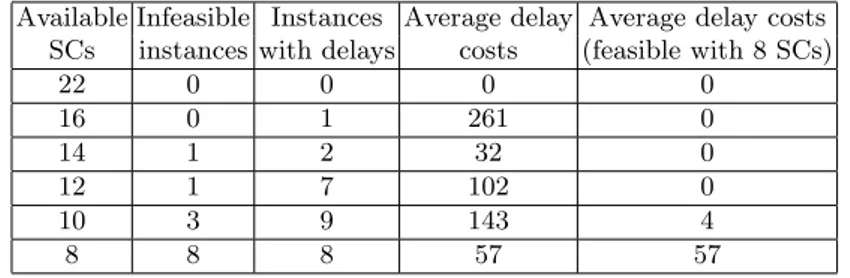
Table 2. Delays for Different Numbers of Available Straddle Carriers Available Infeasible Instances Average delay Average delay costs
SCs instances with delays costs (feasible with 8 SCs)
22 0 0 0 0 16 0 1 261 0 14 1 2 32 0 12 1 7 102 0 10 3 9 143 4 8 8 8 57 57
Experiments are run for 20 instances (days) with different numbers of avail-able straddle carriers (22, 16, 14, 12, 10 and 8) for each instance. The instances are solved using the commercial solver IBM ILOG CPLEX 12. Each feasible instance is solved in a few seconds. Infeasibility is discovered immediately. In-feasibility may occur if the number of available straddle carriers cannot serve all trucks, barges and vessels within their time windows. The results of these exper-iments are shown in Table 2. The first column indicates the number of available SCs used as input. The second column indicates how many instances are infea-sible for the given number of available resources. As expected, the number of infeasible instances increases as the number of available SCs decreases. Columns 3 to 5 present the delays for the feasible instances. Remember that delays are defined differently for each transport mode. For trucks and barges, each period the vehicle spends at the terminal (waiting and service) is penalized. For trains, unexecuted tasks are penalized. For vessels, each shift working on the vessel is penalized. To interpret the results, it must be noted that instances with large delays for a given number of available SCs may become infeasible for a smaller number of available SCs. This has impacts on the measured delays. The third column shows for how many instances delays occur. The fourth column presents the average delay costs for instances with delays. These delays highly depend on the number of feasible instances. Therefore, delays for different number of SCs can hardly be compared. The last column shows the average delay costs only for those instances that are feasible with eight SCs. As expected, decreasing the number of available SCs leads to larger delays.
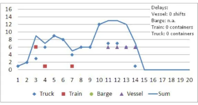
Figures 3 and 4 illustrate two resource allocations proposed by the optimiza-tion model for 14 and 10 available SCs, respectively, for an instance with 1 vessel, 0 barge, 1 train and 580 trucks. The x-axis represents the discrete time periods of the working day. The y-axis represents the number of allocated resources. Both figures show how many resources should be allocated to the different transport modes (truck, train, barge, vessel) at each period of the working day. They also indicate the total number of allocated resources per period. For 14 SCs, the train is served at periods 3, 5 and 7 and the vessel from periods 11 to 14. All trucks are served during the period in which they arrive. Since no barges arrive, no resources are allocated to barges. From periods 10 to 13, more than 10 SCs are on duty. If the number of available SCs is reduced to 10, some tasks executed
Fig. 3. Resource Allocation for 14 Available SCs
Fig. 4. Resource Allocation for 10 Available SCs
in these periods have to be executed in other periods. The vessel is then served in periods 15 to 17 and the train in period 3. Nevertheless, it is not possible to serve all trucks in their arrival periods and delays occur for 15 trucks.
This discussion shows how the model’s output indicates a possible resource allocation minimizing delays. It also illustrates how the model may be used to determine the number of SCs needed for the next working day for the expected workload. For this purpose, the model should be executed for the expected work-load several times with different numbers of available SCs. Results indicate pos-sible resource allocations but also the number of expected delays. The terminal operator may then determine the number of needed SCs for a desired service quality. Remember that SCs are driven by dockers and that the capacity may thus vary from day to day.
7
Conclusion
In this paper, we deal with the allocation problem of internal container han-dling equipment (straddle carriers) at container terminals. Our objective was to determine a resource allocation minimizing vehicle delays. Terminals serve vessels, trucks, trains and barges with adapted service strategies. We presented
a notation to describe the service strategy used at terminals for different trans-port modes. We formulated a modular mixed integer linear program based on a network flow model for the resource allocation problem at container terminals. For each transport mode, a submodel is implemented respecting its character-istics. To represent the entire terminal, these independent submodels may be easily combined. We presented parts of the model implementation for a con-tainer terminal at the “Grand Port Maritime de Marseille”. We discussed some experiments carried out for this terminal to determine an allocation of available resources to different transport modes and to determine the number of resources required to serve the expected demand with a desired service level.
In continuation of this work, the model may be used at tactical and strategic levels. At a tactical level, the model allows the benefits of a shared resource allocation to be analyzed. Different priority rules between trucks, trains, barges and vessels may also be compared. Benefits of an increasing number of tasks that can be handled per resource can also be evaluated. Such an increase may for example result from a more efficient yard organization, shorter travel distances or better trained workers. At a strategic level, the model may be used to analyze the impact of an increasing volume of containers being transported via trains and barges. This transfer from road to rail and waterways is a general aim of today’s logistics. Another possible application is to determine the number of SCs that will be necessary in future to cope with the forecasted demands. Another interesting perspective is to analyze the impacts of the possibility to forward or delay arrivals of vehicles on the number of necessary resources and delays. The model may also be coupled with a scheduling and routing problem to replace the average number of movements per SC per shift by a travel and handling times.
Acknowledgments Part of this work has been conducted within the ESPRIT project, financed by the Mission Transports Intelligents of the DGITM (Direction G´en´erale des Infrastructures, des Transports et de la Mer) of the MEEDDM (Minist`ere de l’Ecologie, de l’Energie, du D´eveloppement Durable et de la Mer). The authors would like to thank Christophe Reynaud, from Marseille Gyptis International.
References
1. Alessandri, A., Cervellera, C., Cuneo, M., Gaggero, M.: Nonlinear Predictive Control for the Management of Container Flows in Maritime Intermodal Terminals. In: 47th IEEE Conference on Decision and Control, pp. 2800–2805. IEEE Press, New York (2008)
2. Das, S.K., Spasovic, L.: Scheduling Material Handling Vehicles in a Container Ter-minal. Production Planning & Control 14, 623–633 (2003)
3. Gambardella, L.M., Mastrolilli, M., Rizzoli, A.E., Zaffalon, M.: An Optimization Methodology for Intermodal Terminal Management. Journal of Intelligent Manu-facturing 12, 521–534 (2004)
4. Hartmann, S.: A General Framework for Scheduling Equipment and Manpower at Container Terminals. OR Spectrum 26, 51–74 (2004)
5. Kang, S., Medina, J.C., Ouyang, Y.: Optimal Operations of Transportation Fleet for Unloading Activities at Container Ports. Transportation Research Part B 42, 970–984 (2008)
6. Notteboom, T., Winkelmans, W.: Factual Report on the European Port Sector. Report commissioned by European Sea Ports Organisation (ESPO) (2004) 7. Vis, I.F., de Koster, R., Savelsbergh, M.W.P.: Minimum Vehicle Fleet Size Under
Time-Window Constraints at a Container Terminal. Transportation Science 39, 249– 260 (2005)
8. Zehendner, E., Rodriguez Verjan, G.L., Absi, N., Dauz`ere-P´er`es, S., Feillet, D.: Optimizing and Simulating Transport Vehicle Allocation in a Multimodal Container Terminal. Working Paper EMSE CMP-SFL (2011)