HAL Id: hal-02930466
https://hal.archives-ouvertes.fr/hal-02930466
Submitted on 4 Sep 2020
HAL is a multi-disciplinary open access
archive for the deposit and dissemination of
sci-entific research documents, whether they are
pub-lished or not. The documents may come from
teaching and research institutions in France or
abroad, or from public or private research centers.
L’archive ouverte pluridisciplinaire HAL, est
destinée au dépôt et à la diffusion de documents
scientifiques de niveau recherche, publiés ou non,
émanant des établissements d’enseignement et de
recherche français ou étrangers, des laboratoires
publics ou privés.
Jason Brown, François Pessaux
To cite this version:
Jason Brown, François Pessaux. Interval-Based Simulation of Zélus IVPs Using DynIbex. Acta
Cyber-netica, University of Szeged, Institute of Informatics, In press, pp.1 - 16. �10.14232/actacyb.285246�.
�hal-02930466�
Interval-Based Simulation of Zélus IVPs Using
DynIbex
∗
Jason Brown
a, François Pessaux
bAbstract
Modeling continuous-time dynamical systems is a complex task. Fortu-nately some dedicated programming languages exist to ease this work. Zélus is one such language that generates a simulation executable which can be used to study the behavior of the modeled system. However, such simulations can-not handle uncertainties on some parameters of the system. This makes it necessary to run multiple simulations to check that the system fulfills partic-ular requirements (safety for instance) for all the values in the uncertainty ranges. Interval-based guaranteed integration methods provide a solution to this problem. The DynIbex library provides such methods but it requires a manual encoding of the system in a general purpose programming language (C++). This article presents an extension of the Zélus compiler to generate interval-based guaranteed simulations of IVPs using DynIbex. This extension is conservative since it does not break the existing compilation workflow. Keywords: DynIbex, Zélus, Compilation, Hybrid System, Interval, Guaran-teed Integration, Simulation
1
Introduction
Hybrid systems are commonly defined as dynamical systems mixing discrete and continuous times. They are widely present in control command systems where a continuous physical process is controlled by software components which run at dis-crete instants. The implementation of such software components involved in many critical systems has to be verified to ensure that the behavior of the global system does not lead to any critical event. One of the verification techniques is to simulate the global system. In such a simulation process, the continuous physical process is
∗This research benefited from the support of the “Chair Complex Systems Engineering - École
Polytechnique, THALES, DGA, FX, DASSAULT AVIATION, DCNS Research, ENSTA Paris-Tech, Télécom ParisParis-Tech, Fondation ParisTech and FDO ENSTA” and it is also partially funded by DGA AID. We warmly thank Julien Alexandre dit Sandretto, Alexandre Chapoutot and Olivier Mullier for the many discussions we had to achieve this work.
aUniversity of Melbourne, E-mail: [email protected] bU2IS, ENSTA Paris, E-mail: [email protected]
modeled as differential equations whose solutions are approximated by dedicated integration algorithms. The discrete processing is the software components. Both parts of the system have to interact, allowing the discrete process to react to events of the continuous one.
Simulations can be very dependent on the initial conditions of the system. Small variations may have important impacts. Moreover, the initial conditions may not always be accurately known. A solution to address these uncertainties is to compute using intervals, hence to rely on interval-based integration tools [10, 14, 2, 3, 4, 17] possibly with guaranteed arithmetic [5, 8, 13].
Domain Specific Languages and tools exist to ease the modeling, development and verification of hybrid systems (Modelica, Simulink/Stateflow, LabVIEW, Zélus and others [7]). These languages provide numerous advantages compared to a manual implementation requiring to explicitly bind the code of the software com-ponents with the runtime/library of simulation. They often propose high-level constructs (automata, differential equations, guards) with dedicated static verifi-cations (typechecking, initialization analysis, scheduling, causality analysis) and compile the hybrid model to low-level code (C, C++) to produce an executable simulation.
This work proposes to bind the flexibility of a hybrid programming language, Zélus[6], with the safety of interval-based guaranteed integration using DynIbex[1, 9]. Zélus natively generates imperative OCaml code linked with a point-wise simulation runtime. DynIbex is a plug-in of the C++ Ibex library, bringing various validated numerical integration methods to solve Initial Value Problems (IVPs). We do not address the compilation of arbitrary Zélus programs toward DynIbex. We present instead the compilation schema for an IVP described in a subset of Zélus to a C++ simulation code using DynIbex. An example is presented, showing the results obtained with the standard Zélus simulation and with the interval-based one.
The rest of the paper is organized as follows. In Section 2, we briefly present Zélus and the features we handle. Section 3 provides a quick introduction to DynIbex and demonstrates how to encode an IVP using the library. Section 4 addresses the compilation schema. Experimental results are described in Section 5. Section 6 is devoted to related work and we conclude and comment on possible further works in Section 7.
2
Zélus Succinctly, Used Features
Zélus is a synchronous programming language extended with ordinary differential equations (ODEs). It provides a wide range of features like synchronous dataflow equations, hierarchical automata, signals, data-types, pattern-matching, functional features, etc. In this paper, we will only address the constructs required to im-plement IVPs. Zélus makes it possible to model systems in which there is an interaction between discrete-time and continuous-time dynamics. In this work, we do not address any discrete-time behavior.
equations relating the inputs and outputs of each node. A node can be instantiated in another one to import the equations of the former in the latter, where parameters are replaced by the effective arguments provided at the instantiation point. This mechanism allows the reuse of sets of equations with different parameters. An IVP is represented by a system of coupled equations coming from the equations defined in a node and those imported from instantiated nodes.
The model of a simple harmonic oscillator with dampening, described by the equation ¨x + k2x + k˙ 1x = 0 with initial values x(0) = 1, ˙x(0) = 0, can be written in
Zélus as:
l e t hybrid shm_decay ( x0 , x ’ 0 , k1 , k2 ) = x where rec der x = x ’ i n i t x0
and der x ’ = −. k1 ∗ . x −. k2 ∗ . x ’ i n i t x ’ 0 l e t hybrid main ( ) = y where
y = shm_decay ( 1 . 0 , 0 . 0 , 4 . 0 , 0 . 4 )
where der x represents ˙x and der x’ is ¨x. The node main instantiates the node shm_decay with specific initial values and k1 and k2. Note that floating-point
arithmetic operators are suffixed by a dot in Zélus.
3
DynIbex in a Few Words, Used Features
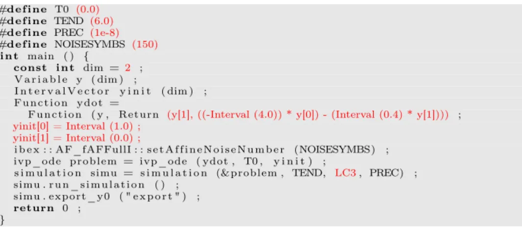
DynIbex is a C++ library that builds on the Ibex library. Ibex provides tools to develop programs for constraint processing over real numbers using interval arith-metic and affine aritharith-metic. DynIbex adds validated numerical integration methods (including handling of floating-point rounding errors). To describe an IVP one de-fines objects of predefined classes to represent the initial values and the ODEs of the system, using vector-valued representation. That is, initial values are a vector of intervals and the ODEs are “merged” into one unique function whose domain and codomain are vectors of intervals. Once these objects are defined, a dedicated func-tion is called to perform the simulafunc-tion with the desired parameters (integrafunc-tion method, duration, precision, etc.).
Using the example introduced in Section 2, we show in Figure 1 the expected result of the compilation into C++ code, where the red parts represent code de-pendent on the compiled IVP. After instantiation of the node shm_decay with the effective arguments, the set of equations is der x = x′
init 1 and der x′
= −4x − 0.4x′
init 0.
The variable dim represents the number of equations of the system, y represents the continuous state of the system, ydot encodes the differential equations in the Return expression. The mapping from the coupled equations x and x’ to the vector-valued representation assigns x to the dimension 0 (y[0]) and x’ to the dimension 1 (y[1]). All the numerical constants are transformed into single-point intervals taking rounding issues in account. If a float cannot exactly be represented, the obtained interval is the smallest containing this float. The initial conditions of the problem are stored in yinit. The number of noise symbols is set using setAffineNoiseNumber. An IVP object problem is created to group the initial
#define T0 (0.0)
#define TEND (6.0)
#define PREC (1e-8)
#define NOISESYMBS (150)
int main ( ) {
const int dim = 2 ; V a r i a b l e y ( dim ) ;
I n t e r v a l V e c t o r y i n i t ( dim ) ; F u n c t i o n y d o t =
F u n c t i o n ( y , Return (y[1], ((-Interval (4.0)) * y[0]) - (Interval (0.4) * y[1]))) ;
yinit[0] = Interval (1.0) ; yinit[1] = Interval (0.0) ;
i b e x : : AF_fAFFullI : : s e t A f f i n e N o i s e N u m b e r (NOISESYMBS) ; ivp_ode p r o b l e m = ivp_ode ( ydot , T0 , y i n i t ) ;
s i m u l a t i o n simu = s i m u l a t i o n (&problem , TEND, LC3, PREC) ; simu . r u n _ s i m u l a t i o n ( ) ;
simu . e x p o r t _ y 0 ( " e x p o r t " ) ; return 0 ;
}
Figure 1: IVP encoding in DynIbex (targeted generated C++ code) values, the equations and the initial time. A simulation object simu is created and run. Finally, the results are exported as plain text, providing for each time interval of the simulation the intervals representing the solution of each equation.
4
Compiling an IVP
4.1
Overview
For several reasons, it is impossible to simply rewrite Zélus’s backend to make it generate C++ code instead of OCaml code and get hybrid systems for free with DynIbex.
First, the generated OCaml code is tightly dependent on the ODE solver used by Zélus and the solving runtime is very different from DynIbex’s mechanisms. Sec-ond, the runtime simulation code is deeply mixed with the IVP problem code, making impossible to distinguish between code to be translated into C++, code to be transformed into intervals and code which should be ignored. Finally, intervals are strongly incompatible with point-wise simulation. General Zélus programs may contain discrete code running on events, using continuous values. When working with intervals, these values are no longer exact which makes, for instance, condi-tional constructs fuzzy : a test may be true and false at the same time. In such a situation, a usual computation cannot be carried out anymore.
For these reasons, we need a dedicated compilation schema to bind Zélus and DynIbex and decide to address only IPV in this work.
In this context, compiling the Zélus code requires two steps. First, the hierar-chy of nodes must be flattened, harvesting all the differential equations and their initial values. During this process, each node instantiation expression is replaced by the body of the node where the occurrences of its parameters are replaced by the effective expressions provided at the instantiation point. This process implies a recursive inlining mechanism which terminates since Zélus forbids recursive nodes.
Since DynIbex simulation only accepts a system of differential equations as input, regular dataflow equations must be transformed into differential equations by sym-bolic differentiation.
Once the intermediate representation of the flattened system is obtained, the multiple equations have to be aggregated into a unique vector-valued function to finally generate the C++ code. Each differential equation corresponds to one dimen-sion of the DynIbex Function data-structure. Initial conditions are also transformed into interval vectors. During this process, Zélus expressions are compiled to C++ expressions. Since nodes are flattened, leading to a list of equations, this process mostly consists of a translation of arithmetic expressions into C++, mapping the identifiers to the appropriate vector component, and converting real constants into trivial proper rounded intervals (i.e. the smallest interval containing the translated float).
4.2
Compiling to the Intermediate Representation
The restricted syntax of programs addressed in this work is given in Figure 2.
p ∶∶= n+
Program n ∶∶= hybrid f (x∗
) = y where eq+
Node
eq ∶∶= der x = e1init e2 Differential equation
∣ x= e Regular dataflow equation e ∶∶= r Real numeric constant
∣ x Identifier
∣ e1 op e2 Arithmetic expression
∣ f(e∗)
Node instantiation
Figure 2: Syntax subset of Zélus for IVP
A program p is a list of nodes. A node n is the definition of a parameterized component returning a value y which is the result of one of the equations eq defined in this node. An equation eq may be a differential equation with an initial value e2or
a regular dataflow equation binding an expression e to an identifier x. Expressions are numeric constants, identifiers, arithmetic expressions or the instantiation of a node named f with expressions. Node instantiations cannot be self-recursive.
The elaboration of the intermediate representation of an IVP proceeds recur-sively on the Abstract Syntax Tree of the program. The inlining pass relies on an environment E, a partial function from node names to node descriptions. We note ⟪n, d ⟫ the environment mapping the node name n to its description d and use the + symbol to denote the addition of a new binding to an environment. A node description is a triplet (I, y, E ) where I is the list of the node’s formal parameters, y is the output of the node (i.e. the name of one of its equations), E is the list of ivpeqs describing the ODEs of the node. An ivpeq is a triplet ⟨ x, e1, e2⟩where x is the name of the differential equation, e1is its expression and e2is its initial value.
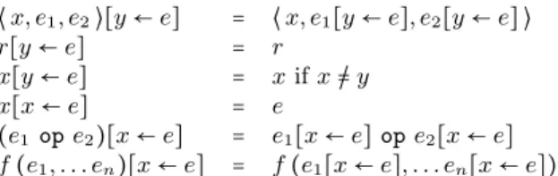
The node instantiation inlining requires a substitution operation on expressions and ivpeqs. Such a substitution is a partial application with a finite domain from
identifiers to expressions. We denote by [x1←e1; . . . ; xn←en]the substitution of the domain {x1, ⋯, xn}associating the expression eito the identifier xi. We extend
a substitution to an application from expressions to expressions and from ivpeqs to ivpeqs as described in the figure 3.
⟨ x, e1, e2⟩[y ← e] = ⟨ x, e1[y ← e], e2[y ← e] ⟩ r[y ← e] = r x[y ← e] = x if x /= y x[x ← e] = e (e1 op e2)[x ← e] = e1[x ← e] op e2[x ← e] f(e1, . . . en)[x ← e] = f (e1[x ← e], . . . en[x ← e])
Figure 3: Substitution in an ivpeq and expressions
Figure 4 gives an example of the inlining process. In gray is the Zélus code. When processing the node foo no changes occur since it contains no instantiation expression. The node bar contains two instantiations. For each of them we import the contents of the node where the formal parameters have been replaced by the effective arguments of the instantiation. Then we add this new equation and we replace the instantiation expression by the name of this new equation. Note that to avoid name conflicts, equations are renamed during this process.
l e t hybrid f o o ( a , b , c ) = v where der v = −9 . 8 − c ∗ a i n i t b foo: v0, v1, v2 -> v3
der v3 = -9.8 - (v2 * v0) init v1
l e t hybrid bar ( y , z , k ) = ( x1 ) where
rec der x2 = f o o ( x2 − x1 , 0 , k + 0 . 5 ) i n i t 2 + 3 and der x1 = f o o ( x2 ∗ x1 , z , k ) i n i t y bar: v0, v1, v2 -> v4 der v3 = v5 init (2 + 3) der v4 = v6 init v0 der v5 = -9.8 - ((v2 + 0.5) * (v3 - v4)) init 0 der v6 = -9.8 - (v2 * (v3 * v4)) init v1 l e t hybrid main ( ) = x where
x = bar ( 1 , (1 / 2) , 3 . 1 4 ) main: -> v0 der v0 = v3 init 1 der v1 = v2 init (2 + 3) der v2 = -9.8 - ((3.14 + 0.5) * (v1 - v0)) init 0 der v3 = -9.8 - (3.14 * (v1 * v0)) init (1 / 2)
Figure 4: Node instantiation inlining example
Since the Function class of DynIbex can only encode ODEs, it is impossible to directly express the equations for u or v in the following example.
hybrid f o o ( ) = u where rec der z = u i n i t 3 . 0 and u = 5 . 0 +. z +. v and v = 1 . +. z
We cannot simply inline the body of u at each occurrence in the equations since u is the return identifier of the node. The solution is to symbolically differentiate 5 + z + v, i.e. create the expressions corresponding to δ(5 + z + v) and the initial
value of 5 + z + v. Inside this expression, the identifier z represents an ODE, so its derivative is exactly the body of z. However, v represents a regular dataflow equation. Hence v must be replaced by the (recursive) differentiation of its body. Thus, the whole equation is replaced by der u = 0 + u + 0 + u. The initial value of this new equation is the original body of u in which z is replaced by the initial value of der z and v is replaced by its body in which we recursively apply the transformation. The obtained result is init 5 + 3 + 1 + 3. In summary, while processing a node definition, any equation defined by y = e must be replaced by der y = B (e) init I (e) where B (e) and I (e) are given in Figure 5.
B (r) = 0
B (e1+ e2) = B (e1) + B (e2)
B (e1∗ e2) = B (e1) ∗ e2 + e1 ∗ B (e2)
B (e1/ e2) = (B (e1) ∗ e2 − e1 ∗ B (e2)) / (e2∗ e2)
B (x) = e1 if x is defined by der x = e1 init e2
B (x) = B (e) if x is defined by x = e I (r) = r
I (e1+ e2) = I (e1) + I (e2)
I (e1∗ e2) = I (e1) ∗ I (e2)
I (e1/ e2) = I (e1) / I (e2)
I (x) = e2 if x is defined by der x = e1 init e2
I (x) = I (e) if x is defined by x = e
Figure 5: B (e) and I (e) rules
The compilation rules for expressions are given in Figure 6. The judgment E ⊢ e1→4(e2, D) means that, in the environment E, the expression e1 is transformed
into the expression e2 and produces the set of ivpeqs D.
(Num) E⊢ r →4(r, ∅) (Id) E⊢ x →4(x, ∅) (App) E(f) = ({x1, . . . , xn}, y, {⟨ d1⟩, . . . , ⟨ dm⟩}) E⊢ e1→4(e ′ 1, D1) . . . E ⊢ en→4(e ′ n, Dn) d′ 1= d1[xi← e ′ i]i=1...n . . . d ′ m= dm[xi← e ′ i]i=1...n E⊢ f (e1, . . . , en) →4(y, {⟨ d ′ 1⟩, . . . , ⟨ d ′ m⟩} ∪ D1∪ . . . ∪ Dn) (Op) E⊢ e1→4(e ′ 1, D1) E ⊢ e2→4(e ′ 2, D2) E⊢ e1op e2→4(e ′ 1op e ′ 2, D1∪ D2)
Figure 6: Compilation of expressions
The rule Num handles a real numeric constant and produces the same constant with an empty set of ivpeqs. The rule Id handles identifiers the same way. The rule App handles the node instantiation and is in charge of the effective inlining. The name f is expected to be bound in the environment to a node description. The expression returned by the rule App is the identifier naming the output of f and the ivpeqs set is the one of f in which all the occurrences of the formal parameters xi of f have been substituted by the corresponding effective argument
expressions e′
all the identifiers of the inlined node by fresh variables (i.e. not appearing anywhere in the program). This renaming is mandatory to avoid variable capture. Finally, the rule Opp recursively processes the two sub-expressions to rebuild an arithmetic expression and the union of the ivpeqs obtained for each sub-expression.
The compilation rules for equations are given in Figure 7. The judgment E ⊢ eq →3Dstates that the equation eq produces the set of ivpeqs D.
(Eq) E⊢ e →4(e ′ , D) eb= B (e ′ ) ei= I (e ′ ) E⊢ x = e →3⟨ x, eb, ei⟩ + D (Der) E⊢ e1→4(e ′ 1, D1) E ⊢ e2→4(e ′ 2, D2) E⊢ der x = e1 init e2→3⟨ x, e ′ 1, e ′ 2⟩ + D1∪ D2
Figure 7: Compilation of equations
The rule Eq handles regular dataflow equations. It transforms the body e of the equation to obtain the ivpeqs representing inlined node instantiation expressions of e. The equation is differentiated and added as a new ivpeq. The rule Der performs the inlining transformation on the body and initial value of the differential equation, and returns the set made of the ivpeqs obtained for each sub-expression extended with the one created for x.
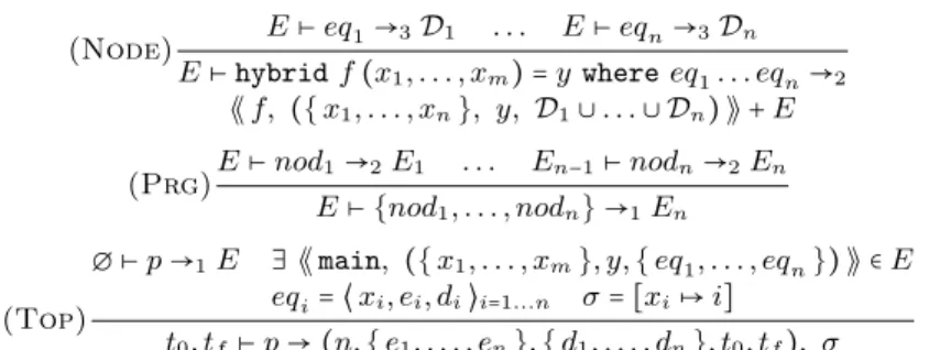
Finally, the compilation rules for nodes then programs are given in Figure 8.
(Node) E⊢ eq1→3D1 . . . E⊢ eqn→3Dn E⊢ hybrid f (x1, . . . , xm) = y where eq1. . . eqn→2 ⟪ f, ({ x1, . . . , xn}, y, D1∪ . . . ∪ Dn) ⟫ + E (Prg) E⊢ nod1→2E1 . . . En−1⊢ nodn→2En E⊢ {nod1, . . . , nodn} →1En (Top) ∅ ⊢ p →1E ∃ ⟪ main, ({ x1, . . . , xm}, y, { eq1, . . . , eqn}) ⟫ ∈ E eqi= ⟨ xi, ei, di⟩i=1...n σ= [xi↦ i] t0, tf ⊢ p → (n, { e1, . . . , en}, { d1, . . . , dn}, t0, tf), σ
Figure 8: Rules for intermediate representation synthesis
The rule Node processes one node, harvesting the ivpeqs obtained from its equations. It returns the environment extended with the node description of f . The rule Prg iterates this process on the list of nodes making the program. The description of each processed node is added to the environment to process the remaining ones. Since Zélus imposes that a node is always defined before any use of it, this ensures that we will always find the node description bound to a node identifier present in an instantiation. The rule Top processes all the nodes of the program p, then looks for a node named main. It builds the representation of the IVP as a tuple containing the size of the problem, the list of ODEs expressions, the list of initial values, the initial (t0) and final (tf) dates of the simulation and
a substitution σ. This substitution maps each identifier binding an equation to an integer representing the rank of its equation. It will be used during the C++ code generation.
Optimization The combination of the instantiation inlining and the differen-tiation process can produce duplicated equations which is inefficient since this in-creases the size of the system. Consider the Zélus program given in Section 2. After the inlining in the node main, we get the set of equations :
der x = x′
init 1 der x′= −4 ∗ x − 0.4 ∗ x′
init 0 y = x
which is transformed during differentiation of y into : der x = x′ init 1 der x′= −4 ∗ x − 0.4 ∗ x′ init 0 der y = x′ init 1
where x and y are redundant. To overcome this inefficiency, when processing equa-tions of the form y = x, we drop the equation and replace y by x in the node (i.e. in its equations and its return value).
4.3
Generating C++ Code
The C++ code generation mostly consists of generating a template like the one shown in Figure 1, where the dimension of the system, the Function object and the initial conditions are instantiated from the intermediate representation of the compiled IVP. Hence, the code generation relies on the intermediate representation of the node main and on some data outside the model (duration, integration method, precision, number of noise symbols) provided at compile-time.
The rule Top already provides the list of initial values and differential expres-sions. Most of what remains is the translation of arithmetic expressions into C++. The substitution σ returned by this rule is used while generating the initial values and the Function object representing the equations. It allows the replacement of identifiers by accesses in the arrays used for DynIbex’s vector-valued representation of the equations. Thus, in the Function object, an identifier x is translated into y[σ (x)]. In the same way, the initial value of x is set in yinit[σ (x)]. A numerical constant n is translated into the trivial interval Interval (n).
5
Experimental Results
We extended the Zélus compiler to implement the described compilation process. This new backend operates on the intermediate representation obtained after type, causality and initialization analyses and does not interfere with the standard com-pilation.
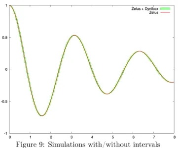
The first experiment was to simulate the system with Zélus and with our gener-ated code, then to compare the results. In Figure 9, the Zélus native simulation is represented by the red line and the simulation obtained using the intervals is shown by the green boxes.
The two simulations behave consistently. In particular, the results obtained with the standard integration runtime of Zélus always remain inside the boxes obtained
Figure 9: Simulations with/without intervals
using the intervals mechanism. This suggests that the native integration runtime of Zélus is precise enough in this example to avoid inaccuracies that could be caused by float rounding errors.
The Zélus syntax has been extended to specify an alternative interval value for any float value. This interval is only taken into account when compiling toward DynIbex. Hence, it is possible to add uncertainty on the initial value of der x, by writing y = shm_decay (1.0 [0.9; 1.0], 0.0, 4.0, 0.4). The “default” value 1.0 is then ignored and the interval [0.9; 1.0] is considered instead. The simula-tion obtained after this change, displayed in Figure 10, shows that both simulasimula-tions continue to behave consistently, but the effect of the uncertainty becomes clearly visible.
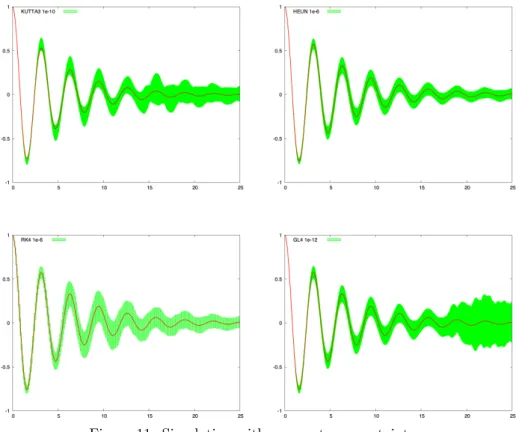
It is also possible to add uncertainty on the coefficients of the equations. The examples in Figure 11 are based on a value of k2 in [0.3; 0.4] instead of 0.4. At
compile-time, it is possible to select different integration methods, precisions, etc. From left to right, top to bottom, we used third-order Runge-Kutta 10−10, Heun’s
method 10−6, fourth-order Runge-Kutta 10−6 and fourth-order Gauss-Legendre
10−12.
Figure 11: Simulation with parameter uncertainty
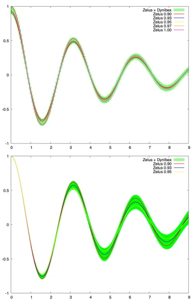
Despite a loss of precision, simulating with intervals to model uncertainties allows one to run one unique simulation instead of several point-wise simulations to try to cover the entire range of uncertainty. The simulation result is less accurate but safe and guaranteed. Running several point-wise simulations is not satisfactory: how many must be ran, which values must be chosen? There is no guaranty that the chosen strategy covers all the possible behaviors. The figure 12 shows the inclusion of several point-wise simulations in a single interval-based simulation. In the top picture, the interval for the initial condition of der x is [0.9; 1]. In the bottom picture, the interval for k2 is [0.3; 0.4]. We plot several point-wise simulations in these ranges of uncertainty. As one expects for safety purposes, the interval-based simulations cover all the point-wise ones.
Figure 12: Point-wise simulations vs interval simulation
6
Related Work
Several frameworks exist for reachability analysis of hybrid systems, though few have a high-level programming language in which to directly describe the systems. JuliaReach [14] is a Julia library performing set-based reachability analysis on both linear and non-linear systems. The description of the system to analyze has to be manually encoded in Julia using the tools provided by the library.
CORA [2] is a toolbox written in MATLAB providing advanced data-structures and reachability algorithms for linear and non-linear systems. It has been extended
with intervals and Taylor models [3, 4]. The modeling of a system is manually done in MATLAB, hence considering floating-point arithmetic as exact.
SpaceEx [10] is a verification platform to model linear (or piece-wise linear) hybrid systems and compute the sets of reachable states using different reachability algorithms. It relies on floating-point arithmetic, though it fails to account for rounding errors. Systems are modeled in a dedicated interface (or in a XML file). A graphical WEB interface is available to set parameters, run simulations and visualize the results. A translator from a subset of Simulink to SpaceEx is also available [16].
FLOW* [8] allows one to model non-linear hybrid systems with uncertainties and compute an over-approximation of reachable states using Taylor models and guaranteed floating-point arithmetic.
Hyson [5] allows one to perform set-based simulations of Simulink hybrid mod-els (continuous and discrete, linear and non-linear, using a subset of the language). It provides guaranteed integration based on Runge Kutta method with handling of floating-point rounding errors. It can be considered as an ancestor of this work.
dReal [11, 12] encodes hybrid systems as SMT modulo ODEs problems. A system has to be encoded as a first-order logic formula with the properties it must respect in the SMT-LIB format. It is then able to check if the properties of the sys-tem hold. However, it does not provide high-level constructs to write the syssys-tems. The Acumen [17, 15] framework provides ways to express various kinds of hybrid systems in a Domain Specific Language. It allows point-wise simulations to provide very fancy dynamic visual representations. It also provides an enclosure interpreter supporting intervals to handle uncertainties for system verification purposes. The main differences with our work come from the nature of the input language and the integration mechanism. Using Zélus provides various static analyses and advanced constructs. Though we do not handle some of these constructs here, work is un-derway to address a larger subset of the Zélus language, including automata, and thus model more complex systems. DynIbex was chosen as a simulation framework as it provides guaranteed integration methods which handles floating-point issues.
7
Future Work
This exploratory work can be extended in three directions. The first direction aims at considering more complex systems. We would like to address IVPs with reset conditions (guards). In such systems, the ODEs are fixed, however the continuous state can be set to particular values on some conditions. To go further, we would like to address systems with several dynamics. In these systems, the ODEs involved in the dynamics may change depending on the state of the system. This will naturally be represented in Zélus by automata. Some obvious issues arise due to the temporal and spacial uncertainties represented by the intervals when changing state in an automaton. Moreover, the compilation schema to implement this will have to remain compatible with the IVPs simulation presented here, while also handling the more elaborate constructs of Zélus.
The second direction is to add contracts in Zélus and to be able to check if they hold during the simulation. First, the form of properties to verify must be chosen since this will have an impact on the logic to use. Then there is the choice of when to verify the contracts: during the simulation or at the end of the simulation. Finally, we need to compile the formulae and represent them with DynIbex constructs.
The last extension of this work is to address the discrete behavior it is possible to model in Zélus. The programs currently supported are restricted to continuous computation. This enables us to model the dynamics of a physical system but not a controller coupled to this system.
8
Conclusion
We presented a mechanism to compile IVPs described in Zélus to C++ code us-ing DynIbex. This allows the simulation of programs written in a high-level pro-gramming language with interval-based validated numerical integration methods. Various parameters can be set at compile-time to tune the simulation accuracy. This work is fully implemented in the Zélus compiler. Extensions to handle more complex systems and to compile contracts verification on programs are in progress.
References
[1] Alexandre dit Sandretto, Julien, Chapoutot, Alexandre, and Mullier, Olivier. The dynibex library.
[2] Althoff, Matthias. An introduction to cora 2015. In Frehse, Goran and Al-thoff, Matthias, editors, ARCH14-15. 1st and 2nd International Workshop on Applied veRification for Continuous and Hybrid Systems, volume 34 of EPiC Series in Computing, pages 120–151. EasyChair, 2015. DOI: 10.29007/zbkv. [3] Althoff, Matthias and Grebenyuk, Dmitry. Implementation of interval arith-metic in CORA 2016. In ARCH@CPSWeek, volume 43 of EPiC Series in Computing, pages 91–105. EasyChair, 2016. DOI: 10.29007/w19b.
[4] Althoff, Matthias, Grebenyuk, Dmitry, and Kochdumper, Niklas. Implemen-tation of taylor models in CORA 2018. In ARCH@ADHS, volume 54 of EPiC Series in Computing, pages 145–173. EasyChair, 2018. DOI: 10.29007/zzc7. [5] Bouissou, Olivier, Mimram, Samuel, and Chapoutot, Alexandre. Hyson: Set-based simulation of hybrid systems. In Proceedings of IEEE Interna-tional Symposium on Rapid System Prototyping, pages 79–85, 2012. DOI: 10.1109/RSP.2012.6380694.
[6] Bourke, Timothy and Pouzet, Marc. Zélus: A synchronous language with odes. In Proceedings of the 16th International Conference on Hybrid Systems: Computation and Control, pages 113–118. ACM, 2013. DOI: 10.1145/2461328.2461348.
[7] Carloni, Luca P., Passerone, Roberto, Pinto, Alessandro, and Angiovanni-Vincentelli, Alberto L. Languages and tools for hybrid systems design. Found. Trends Electron. Des. Autom., 1(1):1–193, 2006. DOI: 10.1561/1000000001. [8] Chen, Xin, Ábrahám, Erika, and Sankaranarayanan, Sriram. Flow*: An an-alyzer for non-linear hybrid systems. In Proceedings of the 25th International Conference on Computer Aided Verification - Volume 8044, CAV 2013, pages 258–263, New York, NY, USA, 2013. Springer-Verlag New York, Inc. DOI: 10.1007/978-3-642-39799-8_18.
[9] dit Sandretto, Julien Alexandre and Chapoutot, Alexandre. Validated explicit and implicit Runge–Kutta methods. Reliable Computing, 22(1):79–103, 2016. [10] Frehse, Goran, Le Guernic, Colas, Donzé, Alexandre, Cotton, Scott, Ray, Rajarshi, Lebeltel, Olivier, Ripado, Rodolfo, Girard, Antoine, Dang, Thao, and Maler, Oded. Spaceex: Scalable verification of hybrid systems. In Ganesh Gopalakrishnan, Shaz Qadeer, editor, Proc. 23rd International Con-ference on Computer Aided Verification (CAV), LNCS. Springer, 2011. [11] Gao, S., Kong, S., and Clarke, E. M. dReal: An SMT solver for nonlinear
theories over the reals. In International Conference on Automated Deduction, volume 7898 of Lecture Notes in Computer Science, pages 208–214. Springer, 2013. DOI: 10.1007/978-3-642-38574-2_14.
[12] Gao, Sicun, Kong, Soonho, and Clarke, Edmund M. Satisfiability modulo odes. CoRR, abs/1310.8278, 2013.
[13] Henzinger, Thomas A., Horowitz, Benjamin, Majumdar, Rupak, and Wong-Toi, Howard. Beyond hytech: Hybrid systems analysis using interval numer-ical methods. In Hybrid Systems: Computation and Control, pages 130–144. Springer Berlin Heidelberg, 2000. DOI: 10.1007/3-540-46430-1_14. [14] Immler, Fabian, Althoff, Matthias, Chen, Xin, Fan, Chuchu, Frehse, Goran,
Kochdumper, Niklas, Li, Yangge, Mitra, Sayan, Tomar, Mahendra Singh, and Zamani, Majid. Arch-comp18 category report: Continuous and hybrid sys-tems with nonlinear dynamics. In Frehse, Goran, editor, ARCH18. 5th Inter-national Workshop on Applied Verification of Continuous and Hybrid Systems, volume 54 of EPiC Series in Computing, pages 53–70. EasyChair, 2018. DOI: 10.29007/mskf.
[15] Konečný, Michal, Taha, Walid, Duracz, Jan, Duracz, Adam, and Ames, Aaron. Enclosing the behavior of a hybrid system up to and beyond a zeno point. In 2013 IEEE 1st international conference on cyber-physical systems, networks, and applications (CPSNA), pages 120–125, United States, 2013. IEEE. DOI: 10.1109/CPSNA.2013.6614258.
[16] Minopoli, Stefano and Frehse, Goran. Sl2sx translator: From simulink to spaceex models. pages 93–98, 04 2016. DOI: 10.1145/2883817.2883826.
[17] Zeng, Yingfu, Rose, Chad G., Brauner, Paul, Taha, Walid, Masood, Jawad, Philippsen, Roland, O’Malley, Marcia K., and Cartwright, Robert. Modeling basic aspects of cyber-physical systems, part II. CoRR, abs/1408.1110, 2014. DOI: 10.1109/HPCC.2014.119.