Frequency approach for detecting nonstationarity in dependent data

Proportions of hits (for test-items T) and false alarms (for similar lures S and different lures D) presented as a function of version (expressive/mechanical) and test item (T),

We aim to use a Long Short Term Memory ensemble method with two input sequences, a sequence of daily features and a second sequence of annual features, in order to predict the next

The analysis results are shown in Fig.1. On average, 62% of used data are in a read-only state but they represent only 18% of the accesses made by the application. The propor- tions

SSN 1 The CLNN model used the given 33 layers of spatial feature maps to predict the taxonomic ranks of species.. Every layer of each tiff image was first center-cropped to a size

The Long Short-Term Memory Deep-Filer (LSTM-DF) was presented in this paper to filter rPPG signals as an al- ternative to conventional signal processing techniques that

We could imagine for instance passing the normalized disparity plane as an extra channel in the cell input and instead of learning features about the most probable color, let

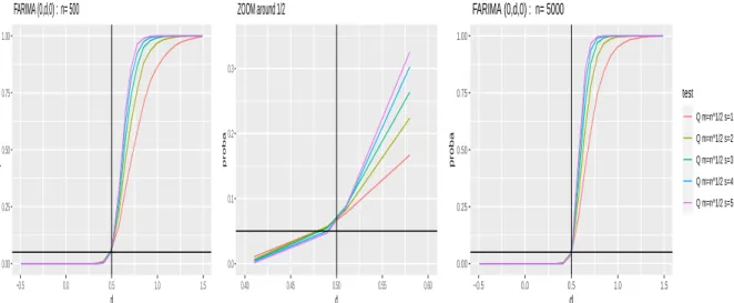
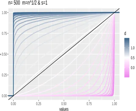
Among all wavelet estimators of the memory parameter d presented in this paper, for a given choice of wavelet and scales involved in the estimates, the estimator with optimal

Central or peripheral blocks allow the delivery of selective subarachnoid anesthesia with local normobaric and/or hyperbaric anesthetics; lipophilic opioids may be used with due

References

Bailey, N. and Giraitis, L. (2016). Spectral approach to parameter-free unit root testing. Comput. Statist. Data Anal., 100:4–16.
Beran, J., Feng, Y., Ghosh, S., and Kulik, R. (2013). Long-memory processes. Springer, Heidelberg. Probabilistic properties and statistical methods.
Deo, R. S. (1997). Asymptotic theory for certain regression models with long memory errors. J. Time Ser. Anal., 18(4):385–393.
Giraitis, L., Koul, H. L., and Surgailis, D. (2012). Large sample inference for long memory processes. Imperial College Press, London.
Giraitis, L., Leipus, R., and Philippe, A. (2006). A test for stationarity versus trends and unit roots for a wide class of dependent errors. Econometric Theory, 22(6):989–1029.
(26)
Gromykov, G., Ould Haye, M., and Philippe, A. (2018). A frequency-domain test for long range dependence. Statistical Inference for Stochastic Processes, 21(3):513–526.
Hu, C., Pozdnyakov, V., and Yan, J. (2020). Density and distribution evaluation for convo-lution of independent gamma variables. Computational Statistics, 35(1):327–342.
Hurvich, C. M. and Beltr˜ao, K. I. (1993). Asymptotics for the low-frequency ordinates of the periodogram of a long-memory time series. J. Time Ser. Anal., 14(5):455–472.
Phillips, P. C. B. and Perron, P. (1988). Testing for a unit root in time series regression. Biometrika, 75:335–346.
R Core Team (2018). R: A Language and Environment for Statistical Computing. R Foun-dation for Statistical Computing, Vienna, Austria.
Shumway, R. H. and Stoffer, D. S. (2017). Time series analysis and its applications with R examples. Springer Texts in Statistics. Springer, fourth edition.
Stoffer, D. (2019). astsa: Applied Statistical Time Series Analysis. R package version 1.9. Taqqu, M. (2003). Fractional brownian motion and long-range dependence. In Theory and
Applications of Long-Range Dependence, pages 5–38. Eds Doukhan, P. and Oppenheim, G. and Taqqu, M. Birkhauser, Boston.
Terrin, N. and Hurvich, C. M. (1994). An asymptotic Wiener-Itˆo representation for the low frequency ordinates of the periodogram of a long memory time series. Stochastic Process. Appl., 54(2):297–307.
Figure
Figure 1: Empirical level evaluated on FARIMA(0,d,0) process as function of the long memory parameter d ∈ (−.5, .5)
Figure 3: Empirical probability to reject the null hypothesis as function of d the parameter of fractional process with d ∈ (−1/2, 3/2)
Figure 4: Empirical cumulative distribution function of the P-value for Q-test for different values of d ∈ (−.5, 1.5)
Références
Documents relatifs