HAL Id: hal-00581815
https://hal.archives-ouvertes.fr/hal-00581815
Submitted on 31 Mar 2011
HAL is a multi-disciplinary open access
archive for the deposit and dissemination of
sci-entific research documents, whether they are
pub-lished or not. The documents may come from
teaching and research institutions in France or
abroad, or from public or private research centers.
L’archive ouverte pluridisciplinaire HAL, est
destinée au dépôt et à la diffusion de documents
scientifiques de niveau recherche, publiés ou non,
émanant des établissements d’enseignement et de
recherche français ou étrangers, des laboratoires
publics ou privés.
Path-Based Distance with Varying Weights and
Neighborhood Sequences
Nicolas Normand, Robin Strand, Pierre Evenou, Aurore Arlicot
To cite this version:
Nicolas Normand, Robin Strand, Pierre Evenou, Aurore Arlicot. Path-Based Distance with Varying
Weights and Neighborhood Sequences. 16th IAPR International Conference, DGCI 2011, Apr 2011,
Nancy, France. pp.199-210, �10.1007/978-3-642-19867-0_17�. �hal-00581815�
Path-Based Distance with Varying Weights and Neighborhood
Sequences
Nicolas Normand1,2, Robin Strand3, Pierre Evenou1, and Aurore Arlicot1
1 IRCCyN UMR CNRS 6597, University of Nantes, France 2 School of Physics, Monash University, Melbourne, Australia
3 Centre for Image Analysis, Uppsala University, Sweden
Abstract. This paper presents a path-based distance where local displacement costs vary both
ac-cording to the displacement vector and with the travelled distance. The corresponding distance trans-form algorithm is similar in its trans-form to classical propagation-based algorithms, but the more variable distance increments are either stored in look-up-tables or computed on-the-fly. These distances and distance transform extend neighborhood-sequence distances, chamfer distances and generalized dis-tances based on Minkowski sums. We introduce algorithms to compute, inZ2, a translated version of
a neighborhood sequence distance map with a limited number of neighbors, both for periodic and aperiodic sequences. A method to recover the centered distance map from the translated one is also introduced. Overall, the distance transform can be computed with minimal delay, without the need to wait for the whole input image before beginning to provide the result image.
@inproceedings{normand2011dgci,
Author = {Normand, Nicolas and Strand, Robin and Evenou, Pierre and Arlicot, Aurore}, Crossref = {dgci2011},
Doi = {10.1007/978-3-642-19867-0_17}, Pages = {199-210},
Title = {Path-Based Distance with Varying Weights and Neighborhood Sequences}} @proceedings{dgci2011,
Address = {Nancy, France},
Booktitle = {Discrete Geometry for Computer Imagery 2011}, Doi = {10.1007/978-3-642-19867-0},
Editor = {Debled-Rennesson, Isabelle and Domenjoud, {\’E}ric and Kerautret, Bertrand and Even, Philippe},
Isbn = {978-3-642-19866-3}, Month = apr,
Publisher = {Springer Berlin / Heidelberg}, Series = {Lecture Notes in Computer Science},
Title = {Discrete Geometry for Computer Imagery 2011}, Volume = {6607},
Year = {2011}}
The original publication is part of the proceedings of the 16th IAPR International Conference, DGCI
Path-Based Distance with Varying Weights and
Neighborhood Sequences
Nicolas Normand1,2, Robin Strand3, Pierre Evenou1, and Aurore Arlicot1
1 IRCCyN UMR CNRS 6597, University of Nantes, France 2 School of Physics, Monash University, Melbourne, Australia
3 Centre for Image Analysis, Uppsala University, Sweden
Abstract. This paper presents a path-based distance where local dis-placement costs vary both according to the disdis-placement vector and with the travelled distance. The corresponding distance transform al-gorithm is similar in its form to classical propagation-based alal-gorithms, but the more variable distance increments are either stored in look-up-tables or computed on-the-fly. These distances and distance transform extend neighborhood-sequence distances, chamfer distances and gener-alized distances based on Minkowski sums. We introduce algorithms to compute, in Z2, a translated version of a neighborhood sequence distance
map with a limited number of neighbors, both for periodic and aperi-odic sequences. A method to recover the centered distance map from the translated one is also introduced. Overall, the distance transform can be computed with minimal delay, without the need to wait for the whole input image before beginning to provide the result image.
1 Introduction
In [8] discrete distances were introduced along with sequential algorithms to compute the distance transform (DT) of a binary image, where each point is mapped to its distance to the background. These discrete distances are built from adjacency and connected paths (path-based distances): the distance between two points is equal to the cost of the shortest path that joins them. For distance d4
(“d" in [8]), defined in the square grid Z2, each point has four neighbors located
at its top, left, bottom and right edges. Similarly, for distance d8 (“d∗" in [8]),
each point has four extra diagonally located neighbors. In both cases, d4 and
d8, the cost of a path is defined as the number of displacements. These simple
distances have been extended in different ways, by changing the neighborhood depending on the travelled distance ([9,2]), by weighting displacements [5,2], or even by a mixed approach of weighted neighborhood sequence paths [10].
Section 2 presents definitions of distances, disks and some properties of non-decreasing integer sequences that will be used later. Section 3 introduces a new generalization of path-based distances where displacement costs vary both on the displacement vector and on the travelled distance. An application is presented in section 4 for the efficient computation of neighborhood-sequence DT in 2D.
2 Preliminaries
Lambek-Moser inverse of a integer sequence [4]. Let the function f de-fine a non-decreasing sequences of integers (f(1), f(2), . . . ) For the sake of sim-plicity, we call f a sequence. The inverse sequence of f, denoted by f†, is a
non-decreasing sequence of integers defined by:
f (m) < n ⇔ f†(n)�< m . (1)
An interesting property of a sequence f and its inverse f†is that, by adding
the rank of each term to these two sequences, we obtain two complementary sequences f(m) + m and f†(n) + n[4]. This property extends the results given
by Ostrowski et al. [7] about Beatty sequences [1]. From [4], we deduce that the inverse of the sequence f(m) = �τm� with a scalar τ, is f†(n) = �n
τ − 1� so
f (m) + m =�(1 + τ)m� and f†(n) + n =�(1 +1τ)n− 1� are two complementary sequences. If τ is irrational, these sequences are Beatty sequences and, for any positive n, �(1 + 1
τ)n− 1� is equal to �(1 + 1
τ)n� as given in [1].
Proposition 1. f†(f (m) + 1) + 1 is the rank of the smallest term greater than
m where f increases. Proof. f†(f (m) + 1) + 1 = m� ⇔ � f†(f (m) + 1) < m� f†(f (m) + 1)≥ m�− 1 ⇔ � f (m�)≥ f(m) + 1 f (m�− 1) < f(m) + 1 ⇔ f(m�) > f (m) and f(m�− 1) ≤ f(m) .
If we extend f with f(0) = 0, and define g by g(0) = 0, g(n + 1) = f†(f (g(n)) +
1) + 1, then f(g(n)) takes, in increasing order, all the values of f, each one appearing once.
Definition 1 (Discrete distance). A function d : Zn×Zn → N is a
translation-invariant distance if the following conditions holds ∀x, y, z ∈ Zn, ∀λ ∈ Z:
1. translation invariance d(x + z, y + z) = d(x, y) ,
2. positive definiteness d(x, y) ≥ 0 and d(x, y) = 0 ⇔ x = y , 3. symmetry d(x, y) = d(y, x) ,
In the following sections, we will drop definiteness and symmetry to define “asym-metric pseudo-distances".
Definition 2 (Disk). The disk D(p, r) of center p and radius r and the sym-metrical disk ˇD(p, r)are the sets:
D(p, r) ={q : d(p, q) ≤ r} , ˇ
Table 1. Example of a non-decreasing sequence f and its Lambek-Moser inverse. f is the cumulative sequence of the periodic sequence (1, 2, 0, 3), f†its inverse. f†(f (n) +
1)+1locates the rank of the next f increase. For instance, f(6) = 9, f†(f (6)+1)+1 = 8 is the rank of appearance of the first value greater than 9, which is 12 in this case.
n 1 2 3 4 5 6 7 8 9 10 11 12 13 14 f (n) 1 3 3 6 7 9 9 12 13 15 15 18 19 21 f†(n) 0 1 1 3 3 3 4 5 5 7 7 7 8 9 f†(f (n) + 1) + 1 2 4 4 5 6 8 8 9 10 12 12 13 14 16
By definition, any disk of negative radius is empty and the disk of radius 0 only contains its center (D(p, 0) =�p�).
Definition 3 (Distance transform). The distance transform DTX of the
bi-nary image X is a function that maps each point p to its distance from the closest background point:
DTX:Zn → N
DTX(p) = min�d(q, p) : q∈ Zn\ X�. (3)
Alternatively, since all points at a distance less than DTX(p) to p belong to
X ( ˇD(p, DTX(p)− 1) ⊂ X) and at least one point at a distance to p equal to
DTX(p)is not in X ( ˇD(p, DTX(p))�⊂ X) then:
DTX(p)≥ r ⇔ ˇD(p, r− 1) ⊂ X . (4)
The DT is usually defined as the distance to the background which is equiva-lent to the distance from the background by symmetry. The equivalence is lost with asymmetric distances, and this definition better reflects the fact that DT algorithms always propagate paths from the background points.
In this paper, we consider path-based distances, i.e. distance functions that associate to each couple of points (p, q), the minimal cost of a path from p to q. For a simple distance, a path is a sequence of points where the difference between two successive points is a displacement vector taken in a fixed neighborhood N , and the cost (or length) of a path is the number of its displacements. The cost of the path (p0, . . . , pn, pn+ v)derives from the cost of the path (p0, . . . , pn):
L(p0, . . . , pn) = r ⇒ ∀v ∈ N , L(p0, . . . , pn, pn+ v) = r + 1 . (5)
Rosenfeld and Pfaltz specifically forbid paths where a point appears more than once [8]. This restriction has no effect on the distance because a path where a point appears more than once can not be minimal. In a similar manner, they exclude the null vector from the neighborhood, forbidding a point to appear several times consecutively. As before, it has no effect on the distance. Notice that, in terms of distance, forbidding a path is equivalent to giving it an infinite cost, so that it can not be minimal. (5) can be rewritten as:
where
cv =
�
1 if v ∈ N ∞ otherwise . For a NS-distance characterized by the sequence B:
L(p0, . . . , pn) = r ⇒ ∀v, L(p0, . . . , pn, pn+ v) = r + cBv(r) , (6)
where the displacement cost cB
v(r)is 1 for a displacement vector in the
neigh-borhood B(r + 1) and infinite otherwise: cBv(r) =
�
1 if v ∈ NB(r+1)
∞ otherwise (7)
For a weighted distance with mask M = {(vk; wk)∈ Zn× N∗}1≤k≤m, the
dis-tance increment only depends on the displacement vector, but not on the disdis-tance already travelled: L(p0, . . . , pn) = r ⇒ ∀v, L(p0, . . . , pn, pn+ v) = r + cv, (8) cv= � w if (v; w) ∈ M ∞ otherwise
Briefly, the displacement cost for a vector v and the travelled distance r, is 1 or ∞, independently of r for simple distances, is equal to 1 or ∞ whether v belongs or not to NB(r)for a NS-distance, is in N∗∪ {∞} according to the chamfer mask
and independently of r for a weighted distance.
In the following, we propose to use a displacement cost, denoted by cv(r),
with values in N∗∪{∞}, that depends both on the displacement vector v and on
the travelled distance r. According to the previous remarks, the cost associated to the null displacement will always be unitary:
∀r ∈ N, c0(r) = 1 . (9)
3 Path-based Distance with Varying Weights
Definition 4 (Path). We call path from p to q, any finite sequence of points P = (p = p0, p1, . . . , pn = q) with at least one point, and denote by P(p, q), the
set of these paths.
Notice that this definition of a path is not related to any adjacency relation. The sequence P = (p) is allowed as a path from p to itself. It is distinct from P = (p, p), the path from p to itself with a null displacement.
Definition 5 (Partial and total costs of a path). Let N be a set of vectors containing the null vector 0 and the positive displacement costs cv(with c0(r) = 1
and cv�∈N(r) =∞). The total cost of the path P = (p0, p1, . . . , pn)is:
where Li(P )is the partial cost of the path truncated to its i + 1 first points (i.e.,
to its i first displacements):
L0(P ) =L(p0) = 0 , (11)
Li+1(P ) =L(p0, . . . , pi+1) =Li(P ) + cpipi+1(Li(P )) . (12)
Definition 6. We use the notation Cvk(r) = r + cvk(r). cvk(r) is the relative
cost of the displacement vk when the distance travelled so forth is r. Cvk(r)
represents the partial cost of the path after this displacement (the absolute cost of this displacement):
Li+1(P ) =Li(P ) + cpipi+1(Li(P )) = Cpipi+1(Li(P )) . (13)
Definition 7. The pseudo-distance induced by ��vk�, cvk
� is defined by: d(p, q) = 0 ⇔ p = q d(p, q) = min P∈P(p,q) � L(P )�.
Definition 8. We call minimal relative (resp. absolute) cost of displacement, denoted by ˆc (resp. ˆC), the quantity ˆcv(r) = min�cv(s) + s− r, ∀s ≥ r�(resp.
ˆ
Cv(r) = min�Cv(s),∀s ≥ r�).
Proposition 2 (Preservation of cost order by concatenation). Appending the same displacement to existing paths preserves the relation order of their costs. Let P = (p1,· · · , pnP) and Q = (q1,· · · , qnQ) be two paths with costs L(P ) and
L(Q), v a vector and P� = (p
1,· · · , pnP, pnP+v), Q�= (q1,· · · , qnQ, qnQ+v)the
extended paths with costs L(P�)and L(Q�)measured with minimal displacement
costs. Then: L(P ) ≤ L(Q) ⇒ L(P�)≤ L(Q�) . (14) Proof. From (13), L(P�) = ˆC v(L(P )) and L(Q�) = ˆCv(L(Q)). By definition of ˆ Cv, s ≤ r ⇒ ˆCv(s)≤ ˆCv(r), which gives (14).
Proposition 3. Let N =�vk�be a set of vectors and, cv(r), the displacement
costs for these vectors. There exists a path P from p to q of cost L(P ) = r measured with costs cv(r)if and only if there exists a path P� from p to q of cost
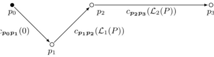
L�(P�) = r measured with the minimal displacement costs ˆc v(r). p0 p1 p2 p3 cp0p1(0) cp1p2(L1(P )) cp2p3(L2(P ))
Fig. 1. Total cost of a path P = (p0, p1, p2). Costs of displacements p0p1, p1p2 and
p2p3 depend on the partial costs L0(P ) = 0, L1(P ) = cp0p1(0) + 0 and L2(P ) =
Proof. Consider the cost of P after i displacements, Li(P ) =Li(p0, p1, . . . , pi),
we note m0 = 1, m0<i≤n = 1 +Li(P )− Li−1(P )− ˆcpi−1pi(Li−1(P )) = 1 +
cpi−1pi(Li−1(P ))− ˆcpi−1pi(Li−1(P )) and Mi =
�i
j=0mi the cumulated sum of
mi. Clearly, if L(P ) is finite then each mi is finite and positive because ˆcv(r)is
less than or equal to cv(r) by construction. Let P� be the (finite) path obtained
by mi occurrences of each point pi:
P�= (p0, p1. . . p1 � �� � m1 , . . . , pi. . . pi � �� � mi , . . . , pn. . . pn � �� � mn ) .
We take as an induction hypothesis that the partial cost of P� after m
i
occur-rences of pi, L�Mi−1(P
�), is equal to L
i(P ). It holds for i = 0 because L�M0−1(P
�) =
L� m0−1(P
�) = L�
0(P�) = 0 = L0(P ). If the hypothesis holds for i − 1, then the
partial cost of P� after the first occurrence of p
i is L�Mi−1(P
�) = L
i−1(P ) +
ˆ
cpi−1pi(Li−1(P )), and after mi− 1 repeats of pi, equals: L�Mi−1+mi−1(P
�) =
L� Mi−1(P
�) =L
i−1(P )+ˆcpi−1pi(Li−1(P ))+mi−1 = Li−1(P )+cpi−1pi(Li−1(P )) =
Li(P )and the hypothesis is true at rank i. Therefore, for every path of finite cost
rmeasured with L, there exists a path with the same cost measured with L�. This is shown in Fig. 2a.
Conversely, let P� be a path with finite cost measured by L�. We build a
path P where each point of P� appears m�
i times consecutively with m�i such
that m�
i− 1 + cpipi+1(L�i(P�) + mi� − 1) = ˆcpipi+1(L�i(P�)). By definition of ˆc,
∀r, ∃s : ˆcv(r) = cv(s)+s−r, so m�iexists. Let M0� = 0and M0<i≤n� =� i−1 j=0mj,
be the cumulated sum of the previous terms of m� i.
The induction hypothesis is that the partial cost of P , measured with L, at the first occurence of pi, LM�
i(P ), is equal to L
�
i(P�). It holds for i = 0 with
a null partial cost LM�
0(P ) = L0(P ) = 0 = L
�
0(P�). If the hypothesis holds at
rank i, the partial cost of P , after m�
i− 1 repetitions of pi, if LM�
i+m�i−1(P ) =
LM�
i(P ) + m
�
i− 1 = L�i(P�) + m�i− 1, and at the first occurence of pi+1, equals
L�
i(P�)+m�i−1+cpipi+1(L�i(P�)+m�i−1) = Li�(P�)+ˆcpipi+1(L�i(P�)) =L�i+1(P�)
and the hypothesis also holds at rank i + 1. An example of such a path is shown on Fig. 2b.
Corollary 1. Displacement costs cv and ˆcv induce the same pseudo-distance.
According to (9), any path from p to q of cost less than r can be extended with null displacements to reach cost r:
L(p0, . . . , pn= q) = s < r ⇒ L(p0, . . . , pn= q, . . . , q
� �� �
1+r−s
) = r (15)
Proposition 4. There exists a path of cost r from p to q if and only if d(p, q) ≤ r.
Proof. If a path of cost r from p to q exists then by definition of the distance, d(p, q) = r if P cost is minimal, d(p, q) < r otherwise. Conversely, if d(p, q) = s then there exists a path of cost s from p to q that, according to (15), can be extended to cost r ≥ s.
(a) p0 p1 p2 +5 +3 +3 +1 +1 +2 +1 r 0 1 2 3 4 5 6 cv(r) 5 2∞ ∞ ∞ 3 1 ˆ cv(r) 3 2 5 4 3 2 1 (b) p0 p1 p2 +3 +4 +1 +2 +1 +1 +1 +1 r 0 1 2 3 4 5 6 cv(r) 5 2∞ ∞ ∞ 3 1 ˆ cv(r) 3 2 5 4 3 2 1
Fig. 2. (a) Given P = (p0, p1, p2), shown with dashed lines, has a total cost L(P ) = 8
measured with displacement costs cv. P� = (p0, p1, p1, p1, p2, p2), solid lines, is built
in such a way that its cost L�(P�) measured with minimal displacement costs ˆcv, is
equal to L(P ) = 8. (b) Given P�= (p
0, p1, p2), shown with solid lines, has a total cost
L�(P�) = 7measured with displacement costs ˆcv. P = (p0, p0, p1, p1, p1, p1, p2), dashed
lines, is built in such a way that L(P ) = L�(P�) = 7.
Corollary 2. For any value of r greater than or equal to d(p, q), there exists a path from p to q which cost is exactly r. The closed disk centered in p with radius r is the set of points for which a path from p of cost equal to r exists:
q∈ D(p, r) ⇔ ∃P ∈ P(p, q), L(P ) = r . (16)
An iterative construction rule of disks is deduced from (16): ∀r > 0, D(p, r) = � v∈N � q : ∃P ∈ P(p, q − v) and Cv(L(P )) = r� = � v∈N s : Cv(s)=r D(p + v, s) (17)
4 Minimal Delay Distance Transform
In [12], Wang and Bertrand, proposed a single scan asymmetric generalized DT based on a neighborhood for which there exists a scanning order such that when a point p in the image is scanned, all neighbors of p have already been scanned (forward scan condition). Then, they extended this result to a sequence where two neighborhoods with forward scan condition are alternated (i.e., B = (1, 2)) [13]. In the following we propose a method to compute an asymmetric generalized DT based on any number of neighborhoods having forward scan condition used in an arbitrary order defined by a sequence B, either periodic or not. For our purpose, we will use translated versions of regular NS-distances neighborhoods, in order to meet the forward scan condition for each of them. The resulting translated distance map can easily be transformed back into a regular, symmetrical, NS-distance map.
Proposition 5. The DT of an image X with the distance induced by the neigh-borhood N and the displacement costs Cv is such that:
DTX(p) =
�
0 if p �∈ X
min� ˆCv(DTX(p− v)), v ∈ N∗� otherwise
(18) where ˆCv represents the minimal absolute displacement costs corresponding to
Cv (definition 8).
Proof. Case p �∈ X directly results from definitions 3 and 7. Suppose now that p ∈ X so any path from q �∈ X to p has at least one displacement. Prop. 3 states that distances induced by ��vk�, Cvk
� and ��
vk�, ˆCvk
� are equal so we consider the latter cost increments for which prop. 2 holds. According to prop. 2, if P = (q = p0, . . . , pn = p− v) is a minimal path from q to p − v then
P�= (q = p0, . . . , pn, p + v)has a minimal cost — among paths from q to p with
second last point p−v — equal to ˆCv(L(P )). So ˆCv(DTX(p− v)) is the shortest
distance from a point q �∈ X to p via p−v. Since all paths which last displacement v does not belong to N have an infinite cost and can not be minimal, (18) holds. 4.1 Generalized Distance Transform
When all vectors in N∗ are directed forward relatively to the scan order, (18)
propagates paths from background pixels in a single scan. As a consequence, a generalized DT using any number of neighborhoods N1. . .Nn, selected by a
sequence B, B(i) ∈ [1, n], derives directly from (7, 18) and minimal costs given by:
ˆ
Cv(r) = min�s : s > rand v ∈ NB(s)�. (19)
let χv(r) denote the characteristic function of the set NB(r) (i.e., χv(r) =
1 if v ∈ NB(r); 0otherwise) and χΣv(r)its cumulative sum (χΣv(r) = � s≤r
χv(r)).
Then according to prop. 1: ˆ
Cv(r) = [χΣv]†(χΣv(r) + 1) + 1 . (20)
Algorithm 1 produces a generalized DT using any sequence of neighborhoods (N represents their union) in forward scan condition, using displacement costs given by (20). A similar algorithm was already presented for the decomposition of convex structuring polygons [6].
4.2 Translated NS-distance transform
The sequence of disks for a NS-distance induced by a sequence B is produced by iterative Minkowski sums of neighborhoods:
Data: X: a set of points
Data: N : neighborhood in forward scan condition Data: ˆCv: minimal absolute displacement costs
Result: DTX: generalized distance transform of X
foreach p in DT domain, in raster scan do if p /∈ X then DTX(p)← 0 else l← ∞ foreach v in N do l← min�l; ˆCv(DTX(p− v)� end DTX(p)← l end end
Algorithm 1: Single scan asymmetric distance transform
For each neighborhood Nj, we apply a translation vector tjsuch that the
trans-lated neighborhood N�
j =Nj⊕�tj�is in forward scan condition. In a translation
preserved scan order, tj translates the first visited point in Nj to the origin.
As-suming a nD standard raster scan order: tj = (0, . . . , 0 � �� � n−j , 1, . . . , 1 � �� � j ) (21)
The translated neighborhoods N�
1 and N2� obtained with t1 = (0, 1) and
t2 = (1, 1) are depicted in Fig. 3a and Fig. 3b. Characteristic functions for
vectors in N�
1\ N2�, N2�\ N1� and N1�∩ N2� (see Fig. 3c-e) are respectively 1B, 2B
and the constant value 1 resulting in the following minimal displacement costs: ˆ Cv(r) = ˆ Cv1(r) = 1†B(1B(r) + 1) + 1 if v ∈ N1� and v �∈ N2� ˆ Cv2(r) = 2†B(2B(r) + 1) + 1 if v �∈ N1� and v ∈ N2� ˆ Cv12(r) = r + 1 if v ∈ N1� and v ∈ N2�
Periodic sequence. When B is a periodic sequence, minimal relative costs ˆcv
are also periodic sequences. Take the periodic sequence of the octagonal dis-tance B = (1, 2), then 1B(r)r≥0 = (0, 1, 1, 2, . . . ), 1†B(r)r>0 = (0, 2, 4, . . . ), ˆ C1 v(r)r≥0 = (1, 3, 3, 5 . . . ) and ˆc1v(r)r≥0 = (1, 2, 1, 2 . . . ). Similarly, 2B(r)r≥0 = (0, 0, 1, 1, 2, . . . ), 2† B(r)r>0 = (1, 3, . . . ), ˆCv2(r)r≥0 = (2, 2, 4 . . . ) and ˆc2v(r)r≥0 = (2, 1, 2, 1 . . . ).
Rate-based sequence. Suppose now that the sequence of neighborhoods is defined as a Beatty sequence (as in [3]): B(r) = �τr� − �τ(r − 1)�, with τ ∈ [1, 2] so that B(r)∈ {1, 2}. 1B and 2B are respectively the cumulative sums of 2 − B(r) =
(a) (b) (c) (d) (e) (f)
Fig. 3. Neighborhoods used for the translated NS-distance transform. (a), and (b) are respectively the type 1 and 2 translated neighborhoods, N�
1 and N2�. (c) and (d) and
(e) are respectively N�
1\ N2�, N2�\ N1� and N1�∩ N2�, each set associated to a different
sequence of displacement costs. (f) is the whole set of neighbors, N�
1∪ N2�, used for the
translated NS-DT. 1 1 1 1 1 1 2 2 2 2 1 1 2 2 2 3 3 2 2 1 1 2 2 2 2 3 4 3 2 1 1 2 1 1 2 2 3 2 2 1 1 1 1 2 2 2 1 1 1 1 1 1 1 1 1 1 1 1 1 1 1 1 1 1 2 2 2 2 1 1 1 1 2 2 2 2 2 2 2 1 1 2 2 2 2 2 3 3 2 1 1 2 2 2 3 3 3 2 2 4 (a) (b)
Fig. 4. (a) Octagonal DT of a binary image. (b) Translated octagonal DT. Highlighted centers of disks (a) are translated to the same location, highlighted (b) with value 3. 1B(r) =�(2 − τ)r�, 2B(r) =�(τ − 1)r�, 1†B(r) =�
r−1
2−τ� and 2†B(r) =� r τ−1− 1�.
This allows to compute ˆC1
v and ˆCv2on the fly. For the octagonal distance, τ = 32,
1B(r) =�r2�, 2B(r) =�r2�, 1†B(r) = 2r− 2 and 2†B(r) = 2r− 1.
An exemple result of algorithm 1 for the translated octagonal distance (with displacement costs obtained either from sequence B = (1, 2) either from τ = 3
2)
is shown in Fig. 4b.
4.3 Symmetric DT from asymmetric DT
Let�t(r), r∈ N∗�be a sequence of translation vectors such that the translated
disks D�(p, r) = D(p + t(r), r) and ˇD�(p, r) = ˇD(p− t(r), r) are increasing
according to the set inclusion. For a sequence of disks produced by translated neighborhoods defined in (21), the translation vectors are:
t(r) = t(r− 1) + tB(r) =� j jB(r)tj = n � j=n jB(r), . . . , n � j=1 jB(r) In particular, for the 2D case:
Data: DT�
X: translated distance map of X
Result: DTX: centered distance map of X
foreach p in DT� domain do if DT�(p) = 0then DT(p)← 0 else foreach j do r← max�1; DT�(p + tj)�
r← j†B(jB(r)) + 1; // First r ≥ DT�(p− tj) such that B(r) = j
while r ≤ DT�(p)do
DT(p− t(r − 1)) ← r
r← j†B(jB(r) + 1) + 1; // Next r such that B(r) = j
end end end end
Algorithm 2: Obtention of a regular (centered) DT from a translated DT.
DT�X has equivalence with values of DTX:
DTX(p)≥ r ⇔ ˇD(p, r− 1) ⊆ X ⇔ ˇD�(p + t(r− 1), r − 1) ⊆ X ⇔ DT�X(p + t(r− 1)) ≥ r . (23) Consequently: DTX(p) = r ⇔ DTX(p)≥ r and DTX(p) < r + 1 ⇔ DT�X(p + t(r))≤ r ≤ DT�X(p + t(r− 1)) . (24) Knowing DT�
X(p)and DT�X(p+t), we can deduce the values of DTX(p−t(r−1))
for all values of r between DT�
X(p + t)and DT�X(p)for which t(r) = t(r − 1) + t,
i.e., t = tB(r). Algorithm 2 recovers the values r of the centered DT by selecting
all r in the interval [DT�
X(p+tj), DT�X(p)]such that B(r) = j. Iterating through
values r with B(r) = j is achieved using prop. 1. Values of DT�
Xbecome available
before the whole image is computed. For instance, in a standard raster scan, as soon as line y is processed, all lines of DT�
X above y − rmaxare fully recovered
(where rmax denotes the maximal value of DT� in that line).
5 Conclusion
In this paper, a path-based pseudo-distance scheme where displacement costs vary both with the displacement vector and with the travelled distance was pre-sented. This scheme is generic enough to describe neighborhood-sequence dis-tances, weighted distances as well as generalized distances produced by Minkow-ski sums. It was shown that a set of displacement costs can be provided in a
minimal form, where each displacement vector is assigned a non-decreasing se-quence of costs, without altering the distance function. These non-decreasing sequences are directly applied in the distance transform algorithm to keep track of the costs of minimal paths from the background. An application to a translated neighborhood-sequence distance transform in a single scan was presented along with a method to recover the proper, centered, distance transform. Combined methods provide partial result with a minimal delay, before the input image is fully processed. Their efficiency can benefit all applications where neighborhood-sequence distances are involved, particularly when pipelined processing architec-tures are involved, or when the size of objects in the source image is limited.
The pseudo-distance presented here is strongly linked to the properties of non-decreasing integer sequences studied by Lambek and Moser. An implemen-tation in C language is publicly available at http://www.irccyn.ec-nantes. fr/~normand/LUTBasedNSDistanceTransform.
References
1. Beatty, S.: Problem 3173. The American Mathematical Monthly 33(3), 159 (Mar 1926)
2. Borgefors, G.: Distance transformations in arbitrary dimensions. Computer Vision, Graphics, and Image Processing 27(3), 321–345 (Sep 1984)
3. Hajdu, A., Hajdu, L.: Approximating the Euclidean distance using non-periodic neighbourhood sequences. Discrete Mathematics 283(1-3), 101–111 (Jun 2004) 4. Lambek, J., Moser, L.: Inverse and complementary sequences of natural numbers.
The American Mathematical Monthly 61(7), 454–458 (Aug-Sep 1954)
5. Montanari, U.: A method for obtaining skeletons using a quasi-Euclidean distance. Journal of the ACM 15(4), 600–624 (Oct 1968)
6. Normand, N.: Convex structuring element decomposition for single scan binary mathematical morphology. In: Nyström, I., Sanniti di Baja, G., Svensson, S. (eds.) DGCI 2003. LNCS, vol. 2886, pp. 154–163. Springer Berlin / Heidelberg, Naples, Italy (Nov 2003)
7. Ostrowski, A., Hyslop, J., Aitken, A.C.: Solutions to problem 3173. The American Mathematical Monthly 34(3), 159–160 (Mar 1927)
8. Rosenfeld, A., Pfaltz, J.L.: Sequential operations in digital picture processing. Jour-nal of the ACM 13(4), 471–494 (Oct 1966)
9. Rosenfeld, A., Pfaltz, J.L.: Distances functions on digital pictures. Pattern Recog-nition 1(1), 33–61 (Jul 1968)
10. Strand, R.: Weighted distances based on neighbourhood sequences. Pattern Recog-nition Letters 28(15), 2029–2036 (Nov 2007)
11. Strand, R., Nagy, B., Fouard, C., Borgefors, G.: Generating distance maps with neighbourhood sequences. In: Coeurjolly, D., Sivignon, I., Tougne, L., Dupont, F. (eds.) DGCI 2008. LNCS, vol. 4992, pp. 295–307. Springer Berlin / Heidelberg, Lyon, France (Apr 2008)
12. Wang, X., Bertrand, G.: An algorithm for a generalized distance transformation based on Minkowski operations. In: International Conference on Pattern Recogni-tion. vol. 2, pp. 1164–1168 (Nov 1988)
13. Wang, X., Bertrand, G.: Some sequential algorithms for a generalized distance transformation based on Minkowski operations. IEEE Transactions on Pattern Analysis and Machine Intelligence 14(11), 1114–1121 (Nov 1992)