Université de Montréal
,ï’7
// 3 q
Q1
Étude photométrique des étoiles naines blanches dans le domaine infrarouge
par
Pier-Emmanuel Tremblay Département de physique Faculté des arts et des sciences
Mémoire présenté à la Faculté des études supérieures en vue de l’obtention du grade de
Maître ès sciences (M.Sc.) en physique
Avril, 2007
J
L
+
L
jUniversité
de Montréal
Direction des bibhothèques
AVIS
L’auteur a autorisé l’Université de Montréal à reproduite et diffuser, en totalité ou en partie, par quelque moyen que ce soit et sur quelque support que ce soit, et exclusivement à des fins non lucratives d’enseignement et de recherche, des copies de ce mémoire ou de cette thèse.
L’auteur et les coauteurs le cas échéant conservent la propriété du droit d’auteur et des droits moraux qui protègent ce document. Ni la thèse ou le mémoire, ni des extraits substantiels de ce document, ne doivent être imprimés ou autrement reproduits sans l’autorisation de l’auteur.
Afin de se conformer à la Loi canadienne sur la protection des
renseignements personnels, quetques formulaires secondaires, coordonnées ou signatures intégrées au texte ont pu être enlevés de ce document. Bien que cela ait pu affecter la pagînation, il n’y a aucun contenu manquant.
NOTICE
The author of this thesis or dissertation has granted a nonexclusive license allowing Université de Montréal to reproduce and publish the document, in part or in whole, and in any format, solely for noncommercia? educational and research purposes.
The author and co-authors
if
applicable retain copyright ownership and moral rights in this document. Neither the whole thesis or dissertation, flot substantia) extracts from it, may be printed or otherwise reproduced without the author’s permission.In compliance with the Canadian Privacy Act some supporting forms, contact
information or signatures may have been removed from the document. While this may affect the document page count, it does flot represent any loss of content from the document.
Ce mémoire intitulé:
Étude photométrique des étoiles naines blanches dans le domaine infrarouge
présenté par:
Pier-Emmanuel Tremblay
a été évalué par unjury composé des personnes suivantes: Cilles Fontaine, président-rapporteur
Pierre Bergeron. directeur de recherche François Wesemael, membre dujury
Sommaire
Il existe maintenant plusieurs ensembles de données dans le domaine infrarouge pour des étoiles naines blanches dont nous présentons une analyse globale. Nous vérifions la fiabilité des observations JHK dans le système CIT, de la base de données du Two Micron Alt Sky Survey (2MASS) et de la photométrie dans l’infrarouge moyen du Spitzer Space Tetescope. Notre méthode d’analyse est la méthode photométrique qui consiste à comparer les flux infrarouges observés, intégrés sur des bandes passantes, aux flux théoriques determinés avec nos modèles d’atmosphère. On utilise d’abord cette méthode avec l’échantillon de 2MASS pour identifier systématiquement les naines blanches binaires avec n compagnon froid de la séquence prin cipale. D’autre part, avec un échantillon d’étoiles froides de 2MA$S, on détermine le ratio du nombre d’étoiles de types non-DA et DA en fonction de la température effective. Cela constitue l’étude avec le plus grand échantillon et la plus grande précision à ce jour. La va riation de ce ratio suggère que le mélange convectif de la couche superficielle d’hydrogène est responsable de la transition d’une faible fraction (-15%) d’étoiles DA vers des non-DA à basse température effective (Teff 9000 K). Finalement, l’analyse de l’évolution spectrale à très basse température effective (Teff < 5000 K) montre que notre connaissance est limitée par l’absence d’un modèle adéquat de l’opacité de l’absorption induite par collisions à hautes densités.
Mots ctefs:
étoiles : binaires — étoiles : mélange convectif — étoiles : modèles d’atmosphère — étoiles paramètres fondamentaux — naines blanches — techniques t photométriques
We present a global analysis of the many infrared photometric data sets available for white dwarfs. We evaluate the reliability of the JHK observations in the OIT system, the Two Micron Alt Sky $nrvey (2MASS) database, and the mid-inftared photometry from the Spitzer Space Tetescope. Our analysis uses the photometric method, which compares the observed infrared fluxes, integrated over bandpasses, to the theoretical fluxes from state of-the-art model atmospheres. We use this method with the 2MASS data set to identify systematically binary white dwarfs with a cool main sequence companion. Secondly, with a 2MASS sample of cool white dwarfs, we determine the ratio of non-DA to DA stars as a function of effective temperature. This study achieves a higher accuracy and uses a larger sample of white dwarfs than any previous analysis. The variation of this ratio suggests that convective mixing of the hydrogen layer is responsible for the transition of a small fraction of DA (‘15%) to non-DA stars at low effective temperatures (Teif ‘-‘ 9000 K). Finally, an
analysis of the spectral evolution at lower effective temperatures (Teff < 5000 K) shows that our knowledge is limited by the lack of accurate opacity calculations of collision induced absorptions (CIA) at high densities.
Subject headings:
stars : binaries stars : convective mixing — stars : fundamental parameters — stars : model atmospheres : — techniques : photometric — white dwarfs
Table des matières
Sommaire i
Abstract ii
Table des matières iii
Liste des figures vi
Liste des tableaux Viii
1 Introduction 1
2 Grille de modèles d’atmosphère 3
2.1 Équation d’état 3
2.2 Opacités 5
2.3 Présentation de la grille 6
3 WHITE DWARFS FROM 2MASS AND THE SPITZER TELESCOPE 8
3.1 ABSTRACT 9
3.2 INTRODUCTION 9
3.3 COMPARISON 0F CIT AND 2MASS PHOTOMETRY 12
3.4 WHITE DWARFS AND LOW MASS MAIN SEQUENCE BINARIES FROM
2MASS 16
3.4.1 The Wachter et al. Analysis 16
3.5 3.6 3.7 3.8 3.9 3.10
4 Étude du mélange convectif
4.1 Définition de l’échantillon de 2MASS
4.2 Détermination des paramètres atmosphériques 4.3 Détermination des incertitudes
4.4 Résultats sur le mélange convectif 4.5 Incertitudes systématiques
4.6 Évolution spectrale entre DA et non-DA .
4.7 Naines blanches binaires
19 22 25 28 30 33 41 50 54 56 59 63 69 71 71
5 Naines blanches absorbant dans 5.1 Observations 5.2 Connaissances actuelles . 5.2.1 Contraintes 5.2.2 Pistes de solutions 73 74 76 77 77 Remerciements 88 Annexe A 89
A Précisions sur l’équation d’état A.1 Ionisation par pression
3.4.3 The Synthetic Flux Method
INFRARED PROTOMETRY FROM SPITZER
CANDIDATE WHITE DWARFS WITH CIRCIJMSTELLAR DISKS CONCLUSION REFERENCES TABLES FIGURES l’infrarouge 6 Conclusion 81 Bibliographie 83 89 89
TABLE DES MATIÈRES
A.2 Quantités thermodynamiques 90
A.3 Illustration de l’équation d’état 90
Annexe B 93
B Échantillon de 2MASS 93
Annexe C 104
2.1 Grille de spectres théoriques 7
3.1 Differences in magnitudes between the infrared CIT and 2MASS photometric
systems for 160 cool white dwarfs 41
3.2 (J — H) vs. (H — K/K) two-color diagrams for our sample 42 3.3 Fits to the optical BVRI and infrared JHK CIT photometric energy distri
butions for selected objects 43
3.4 Same as Figure 3.2 but with the four regions defined by Wellhouse et al. (2005) 44 3.5 Observed and predicted 2MASS fluxes for several binary and tentative binary
candidates from Wachter et al. (2003) 45
3.6 Fits to the energy distribution of white dwarfs from the sample of Kilic et al.
(2006b) 46
3.7 The ratio of observed to predicted Spitzerfluxes for 12 objects from the sample
of Kilic et al. (2006b) 47
3.8 Same as Fig. 3.5 but for the six white dwarfs discussed in
§
5 48 3.9 Differences between the 2MASS observed and predicted (J—H) and (J— Ks)color indices for our sample of massive white dwarfs 49
4.1 La zone convective en terme de la fraction de la masse d’hydrogène en fonction
de Teff 53
4.2 L’échantillon de Sion (1984) 54
LISTE DES FIGURES vii
4.4 La différence de la couleur (V — J) pour des valeurs de logg de 8.5 et 7.5 en
fonction de Teff 58
4.5 Minimisation de la distribution d’énergie VJHK5 pour huit naines blanches
brillantes 60
4.6 La variation de la température effective pour une variation de (V — J) de 0.0$
magnitude en fonction de Teff 61
4.7 Différences entre les températures de notre échantillon et celles déterminées par
BRL97 et BLRO1 62
4.8 Différences entre les températures de notre échantillon et celles déterminées de
façon spectroscopique 64
4.9 Histogramme de la distribution des naines blanches de l’échantillon de 2MASS 65 4.10 Le rapport des volumes sondés pour des naines blanches riches en hélium et en
hydrogène dans un relevé limité en magnitude 66
4.11 Le rapport du nombre d’étoiles riches en hydrogène et riches en hélium en
fonction de Teff 67
4.12 La température effective à laquelle il y aura une mélange convectif pour une
fraction de masse d’hydrogène donnée . 68
4.13 Histogrammes du nombre d’étoiles DA et non-DA avec des mesures de leurs
mouvements propres 70
5.1 Minimisation photométrique de LHS 3250 76
5.2 Modèles avec une équation d’état iion-idéale 78
5.3 Section efficace ad-hoc 79
A.1 Équation d’état dans le plan logP — logp 91
A.2 Équation d’état dans le plan logP — logp (suite) 91
2.1 Espèces chimiques dans l’équation d’état 4
2.2 Types d’opacités 6
3.1 Sample of Cool White Dwarfs with Near-Infrared Photometry 33 3.2 Statistical Comparison of CIT and 2MASS Magnitudes 36 3.3 Sample of White Dwarfs with Predicted NIR Photometry 37
3.4 Sample of Massive White Dwarfs 39
4.1 Comparaison entre températures photométriques et spectroscopiques 59
5.1 Observations de naines blanches absorbant dans l’infrarouge 75
B.1 Échantillon de naines blanches de 2MASS riches en hydrogène 93 B.2 Échantillon de naines blanches de 2MASS riches en hélium 100 B.3 Échantillon de naines blanches binaires riches en hydrogène 102 B.4 Échantillon de naines blanches binaires riches en hélium 103
Chapitre
1
Introduction
Notre compréhension des étoiles naines blanches est contrainte par la seule partie qui est directement observable, soit la couche atmosphérique d’où émerge le flux. La méthode photométrique, qui consiste à comparer les flux théoriques aux flux observés intégrés sur des bandes spectrales, représente un outil d’analyse puissant. Historiquement, l’observation de couleurs (par ex. B — V) a été une ressource importante pour identifier systématiquement les candidats de naines blanches dans des relevés (par ex. PC; Green et al. 1986) et pour estimer leur température effective. Plus récemment, la minimisation photométrique en BVRIJHK, avec des données spectroscopiques pour contraindre la composition et des mesures de la paral laxe pour contraindre la gravité, s’est avérée être la méthode la plus précise pour déterminer les paramètres atmosphériques (température, gravité, composition) des naines blanches froides (Bergeron et al. 1997, 2001). La détermination de ces paramètres dans l’échantillon local de naines blanches permet d’analyser l’évolution chimique des naines blanches froides (Sion 1984; Dufour 2006) ou d’étudier la fonction de luminosité et par conséquent l’âge de la composante locale du disque (Bergeron et al. 1997). En analysant les paramètres des naines blanches les plus froides et leurs données cinématiques, on peut également contraindre la densité locale de la composante dii halo (Bergeron et al. 2005).
Pour les étoiles plus chaudes (Teff 10000 K), la méthode spectroscopique, qui compare les profils théoriques et observés des raies spectrales, s’avère plus efficace pour la détermination des paramètres atmosphériques (Bergeron et al. 1992). Cependant, la méthode photométrique
demeure un outil important. Le fait que l’on sonde le flux du continu sur une large plage de fréquences implique que la méthode photométrique n’est pas sensible aux mêmes processus physiques que la méthode spectroscopique. En particulier, la minimisation photométrique n’est affectée que faiblement par la gravité et on appelle souvent la solution photométrique un indice de températnre, ce qui apporte une contrainte importante sur la solution spectroscopique. De plus, lorsqu’on étudie des naines blanches de différents types spectraux, cette méthode est homogène car elle sonde le continu qui est créé par des processus physiques qui sont bien connus.
On s’intéresse dans cet ouvrage aux ensembles disponibles de photométrie dans le domaine infrarouge de naines blanches. Ceci inclut les données JHK dans le système CIT (Bergeron et al. 1997, 2001) et celles des bases de données du Two Micron Ati Sky $nrvey (2MASS) et du Spi zter Space Tel escope. Ces données sont importantes dans la méthode photométrique puisqu’on augmente la précision en sondant la distribution d’énergie sur une plus grande plage spectrale. De plus, la partie infrarouge du spectre électromagnétique nous permet d’étudier des objets (compagnons froids, disques) ou des phénomènes physiques (absorption infrarouge) qui ne sont pas détectables à plus haute énergie. Cette analyse à grande échelle nécessite des modèles d’atmosphère homogènes pour des naines blanches de températures effectives et compositions arbitraires, ce que nous présentons au chapitre
§
2. D’autre part, le chapitre§
3 analyse la fiabilité des données photométriques infrarouge disponibles. Ayant contraint les limites de l’utilisation des modèles et des données, la deuxième partie de cet ouvrage est consacrée à comparer les données photométriques infrarouge à nos modèles selon trois axes principaux. On présente au chapitre§
3 les contraintes de la recherche de naines blanches binaires et de disques avec les données de 2MASS. Au chapitre§
4, on utilise l’échantillon de 2MA$S pour étudier le mélange convectif dans les naines blanches froides. Finalement, on discute des naines blanches très froides absorbant dans l’infrarouge(
5).Chapitre
2
Grille de modèles d’atmosphère
d’étoiles naines blanches
Notre but est d’analyser la photométrie d’étoiles naines blanches de façon homogène à toutes les températures effectives et pour toutes les compositions. Ainsi, nous avons développé un code de modèles d’atmosphère ETL qui permet de calculer des spectres théoriques pour des températures de 2000 K à 140,000 K, pour un mélange arbitraire d’hélium et d’hydrogène et pour des longueurs d’ondes de 50 à 100000
À.
Nous utilisons comme codes de base celui de Bergeron et al. (1991, 1995, 2001) et références ci-incluses, restreint aux naines blanches froides et le code de Wesemael et al. (1980) restreint aux naines blanches chaudes. Nous avons fait la jonction entre les deux codes en plus de mettre à jour l’équation d’état et les opacités.2.1
Équation d’état
Notre équation d’état fournit les populations de toutes les espèces présentées au Tableau 2.1 pour les variables indépendantes définies comme la température, la pression et la fraction d’hélium et d’hydrogène. Les populations sont calculées par une procédure d’itérations de Newton-Raphson.
Nous utilisons l’équation d’état non-idéale de Hummer & Mihalas (1988) (dorénavant HM88), où on considère la perturbation statistique de chaque atome par ses voisins neutres
CHAPITRE 2. GRILLE DE MODÈLES D’ATMOSPHÈRE 4
TABLEAU 2.1 — Espèces chimiques dans l’équation d’état
Espèce Niveaux
x’
(eV) Rayon (À)H I 16 13.606 [1.$76-0.2941og(T)+(-0.576+0.lOOlog(T)p]n2u
HIl 1-
-H 1 0.755 1.15 b
H2 322 4.478 [2.226-0.3311og (T)+(-0.975+0.1751og (T)p]i(j)
Ht 1 2.650 1.32 b H 1 8.824 0.65 b He I 13 24.587 0.39 (n=1), 2.12 (n=2-5), 4.8 (n=6-11), 8.5 (n=12), 12.5 (n=13) He II 6 54.425 0.39n2 HelIl 1 Hej 1 2.365 1.0 HeH 1 1.961 0.76 C e 1— —
Saumon & Chabrier (1991)
b
Lenzuni & Saumon (1992) Saha et al. (1978)
Les rayons de H et H2 de Saumon & Chabrier (1991) sont valides pour Ïogp < 0, 3.46 < logT < 4.26 et t’(i)
définit le rayon des niveaux de vibrations/rotations par rapport au niveau fondamental (voir l’équation 2.41 de Saumon 1990). Les nombres de niveaux sont seulement ceux dont les populations sont calculées explicitement et diffèrent de ceux considérés dans les fonctions de partitions. Ces dernières sont calculées explicitement ou à partir de tables pour le Ht (Stancil 1994), H (Neale & Tennyson 1995), Het (Stancil 1994), HeH (Engel et al. 2005). Nous négligeons le H qui n’est jamais dominant par rapport au H.
et chargés. En bref, chaque niveau atomique lié possède une probabilité 1 — w d’être détruit par l’interaction avec son environnement. La probabilité w est définie comme w wflwC où
w7 constitue l’interaction avec les particules neutres et w’ l’interaction avec les particules chargées. Pour une espèce liée i dans l’état
j
donné, ces termes prennent la forme= exp +Tk)3) (2.1) 4 tZ 1’h/22 wj = exp
(
—-f16 1/2 e NQZ2)
(2.2) X2,jj
où k et sont des sommes sur les états liés et chargés respectivement, r représente le rayon des états définis dans le Tableau 4.2 et les autres termes sont tels que décrits dans HM$8. La fonction de partition d’une espèce donnée devient alors
Z = wj,jexp
(—)
(2.3)les états excités, une calibration faite à partir des observations de naines DA froides (Teff 8000— 10, 000 K) montrant que le modèle de HM$$ surestime les effets non-idéaux (Bergeron et al. 1991). L’équation d’état résultante du modèle de HM88 est donnée par
= fl+
(
k(Tk + r,)3) +(/
_i)
+
+ (2.4)
où l’indice s représente toutes les espèces (liées ou libres), ji est le potentiel chimique, a est la constante de radiation et
f,
sont les intégrales de Fermi-Dirac. Les termes sont, dans l’ordre d’apparition, la pression du gaz idéal, la pression résultante de l’interaction entre particules neutres, la pression de dégénérescence électronique, la pression de Coulomb’ et la pression de radiation. L’annexe A présente la correction pour permettre l’ionisation par pression, la détermination des quantités thermodynamiques et une illustration des résultats dans l’espace P-p.2.2
Opacités
À
partir des populations determinées précédement, l’opacité totale est calculée à partir des opacités individuelles identifiées dans le Tableau 2.2. Pour les transitions liés et liés-libres de l’hydrogène et de l’hélium, nous utilisons le formalisme de HM8$. La probabilité de transition entre des niveaux liés m et n est multipliée par Bj,m,=(wj,0/uj,m) pour tenir compte de la probabilité que les niveaux en question ne soient plus liés2. Si le niveau supérieur est dissocié, on peut considérer que ce sera une transition du type lié-libre, dont l’amplitude sera Di,m,n=1(wi,n*/wi,m). Le coefficient correspond à la probabilité d’occupation d’un niveau fictifn ayant l’énergie du photon.1Nous utilisons les relations standards pour un gaz neutre et un gaz complètement dégénéré avec une
interpolation entre les deux régimes. Nous négligeons la pression reliée aux interactions des particules chargées (éq. 2.2).
20n négligle le facteur Bi,n,m pour les niveaux de vibrations du H2 dans l’opacité du CIA. Ce facteur vaut
moins de 10% dans le proche infrarouge puisque la différence de rayon entre les niveaux concernés (Saumon 1990) est faible.
CHAPITRE 2. GRJLLE DE MODÈLES D’ATMOSPHÈRE 6
TABLEAU 2.2 — Types d’opacités
Opacité Populations Section efficace
H I lié-lié ni,m(H I)Bi,n,m Lemke (1997)
H I lié-libre 11i,m(H I)Dj,n,m Mihalas (1978)
H I libre-libre nen(H II) Mihalas (197$)
H2 libre-libre nn(H) on suppose celle de H I
H3 libre-libre nen(H) on suppose celle de H I
H lié-libre n(H) John (198$)
H libre-libre nn(H I) John (198$)
Ht libre-libre n(H I)n(H II) Kurucz (1970)
Ht lié-libre n(H)t Kurucz (1970)
H libre-libre nen(H2) Bell (1980)
H quasi-moléculaire n(H I) Allard et al. (1994)
He I lié-lié nj,m(He I)Bi.n,m Beauchamp (1995)
He II lié-lié njm(He II)Bi,n,m Beauchamp (1995)
He I lié-libre n,,m(He I)Dj,,*m Mihalas (1978)
He II lié-libre nj,m(He II)D,,,*,m Mihalas (1978)
He I libre-libre nen(He II) Mihalas (1978)
He II libre-libre nen(He III) Mihalas (1978)
He libre-libre nen(He) John (1968) John (1994)
Het lié-libre n(He) Stancil (1994)
He libre-libre n(He I)n(He II) Stancil (1994)
CIA H-H2 n(H I)n(H2)(1+2x10²³n(H2)) Gustafsson Frommhold (2003)
CIA H2-H2 n(H2)2(1+1.7056x10²³n(H2)) Borysow et al. (2001)
CIA He-H2 n(He I)n(H2)(1±1.8608x10²³n(He I)) Jorgensen et al. (2000)
CIA He-H n(He I)n(H I)(1+2x10²³n(He I)) Gustafsson & frommhold (2001)
Rayleigh H I n(H I) Kissel (2000)
Rayleigh H2 n(H2) Dalgarno& Williams (1962)
Rayleigh He I n(He I) Kissel (2000)
Rayleigh He II n(He II) Kissel (2000)
Thompson e ne Mihalas (197$)
voir (Lenzuni & Saumon 1992) (et références ci-incluses) quant aux corrections pour les collisions à trois corps. Les coefficients pour H-H2 et He-H2 sont une supposition.
Nous négligeons les opacités suivantes qui ne sont jamais importantes pour des naines blanches H2 lié-lié, H
lié-lié et HeH lié-lié.
2.3
Présentation de la grille
Le calcul de l’opacité de Rosseland et la résolution numérique des équations de la structure atmosphérique sont tels que décrits dans Bergeron et al. (1995, et références ci-incluses). Une différence importante se situe au niveau du calcul d’atmosphères complètement radiatives où, pour permettre la convergence, on solutionne une version mixte de l’équation d’équilibre radiatif et de l’équation de conservation du flux.
Pour les naines blanches chaudes, les effets hors-ETL deviennent importants et pour en tenir compte dans les prochains chapitres, nous utilisons la grille de DA hors-ETL telle que décrite dans Liebert et al. (2005). En bref, cette grille utilise nos modèles ETL à basses
températures effectives où les effets hors-ETL sont négligeables et effectue un branchement avec des modèles hors-ETL quand l’atmosphère devient complètement radiative en s’assurant qu’au point de jonction les spectres des deux grilles soient en accord (Teff = 20, 000 K). La
figure 2.1 illustre une partie de notre grille ETL pour des modèles d’atmosphères d’hydrogène et d’hélium. 15 10 Q) X 5
o
0.55FIGuRE 2.1 — Gauche : Illustration de notre grille de spectres théoriques hors-ETL pour une
composition d’hydrogène. Les températures effectives sont identifiées sur la figure en unités de i0 K. L’unité de flux est arbitraire et les spectres sont décalés d’une unité. Droit Même figure mais pour notre grille de spectres avec une composition d’hélium.
B ‘Ï’. 12 10 4— 2
o
0.4 0.5 0.6 0.7 0.35 0.40 0.45 0.50Chapitre
3
INFRARED PHOTOMETRIC ANALYSIS 0F WHITE
DWARFS FROM THE TWO MICRON AIL SKY SURVEY
AND THE SPITZER SPACE TELESCOPE
P.-E. Tremblay’ and P. Bergeron’
Accepted for publication in the The AstTophysicaÏ Journat,
November 2006
1Département de Physique, Université de Montréal, C.P. 6128, Succ. Centre-Ville, Montréal, Québec, Ca nada H3C 3J7; tremb1ayOastro.umontrea1.ca, bergeron(astro.umontrea1.ca
3.1
ABSTRACT
We review the available near- and mid-infrared photometry for white dwarfs obtained from the Two Micron All-Sky Survey (2MASS) and by the Spitzer Space Tetescope. Both data sets have recently heen used to seek white dwarfs with infrared excesses due to the presence of unresolved companions or circumstellar disks, and also to derive the atrnospheric parameters of cool white dwarfs. We flrst attempt to evaluate the reliability of the 2MASS photometry by comparing it with an independent set of published JHK CIT magnitudes for 160 cool white dwarf stars, and also by comparing the data with the predictions of detailed model atmosphere calculations. The possibility of using 2MASS to identify unresolved M dwarf companions or circumstellar disks is then discussed. We also revisit the analysis of 46 binary candidates from Wachter et al. using the synthetic flux method and conflrm the large near-infrared excesses in most objects. We perform a similar analysis by fitting Spitzer 4.5 and 8 m photornetric observations of white dwarfs with our grid of model atmospheres, and demonstrate the reliability of both the SpitzeT data and the theoretical calculations up to 8 /im. Finally, we search for massive disks resulting from the merger of two white dwarfs in a 2MASS sample composed of 57 massive degenerates, and show that massive disks are uncommon in such stars.
3.2
INTRODUCTION
With the recent All-Sky Data Release of the Two Micron All-Sky Survey2 (2MASS), we are
now able to retrieve near-infrared (NIR) J, H, and K3 magnitudes for more than a thousand white dwarfs that fall within the 2MASS detection limit. This database vas used in several studies aimed at identifying new cool white dwarfs (e.g., de La Fuente Marcos et al. 2005) or circumstellar disks (Kilic et al. 2006a) and seeking binary candidates (Wachter et al. 2003; Holberg & Magargal 2005; Debes et al. 2005). In the latter case, one of the main interests are the binary systems containing a main sequence star and a white dwarf. These systems might reveal important details about stellar populations and evolution. Different techniques
CHAPITRE 3. WHITE DWARFS FROM 2MASS AND ITIE SPITZER TELESCOPE 10
have been used to seek these binary candidates. lintil recently, most systematic searches were based on surveys of resolved common proper-motion binaries (Silvestri et al. 2002), but new interest has emerged for identifying unresolved binaries. Que of the reasons is that accretion from a previously unknown close companion could account for the high metal abundances observed in some white dwarfs. The preferred method for seeking unresolved binary candidates is to perform a photometric analysis. In the case where the companion is an M dwarf, the white dwarf star usually dominates the observed flux in the optical regions. Therefore, h is natural to look for an excess in the NIR, either photometrically or spectroscopically, where the contribution from the M dwarf becomes dominant (see Dobbie et al. 2005, for a review).
Exploiting the 2MASS photometric data, different methods of analysis were used to iden tify NIR excesses. Wachter et al. (2003) used the second incremental 2MAS$ data release, which covers about 50% of the sky. The authors took the approach of a (J — H, H — Ks) two-color diagram for 795 white dwarfs recovered from the 2MASS survey. They identifled 95 binary candidates. including 47 objects with prior evidence of binarity. They also suggested 15 additional tentative binary candidates. Wellhouse et al. (2005) used a similar two-color diagram approach with a sample of 51 magnetic white dwarfs as candidates for potential pre-cataclysmic variables. Whule they did not find any binary candidates, they identifled 10 objects with peculiar colors associated with very low mass companions or debris. Holberg & Magargal (2005) used the final 2MASS All-Sky Data Release to study the 347 DA stars from the Palomar-Green Survey (Liebert et al. 2005). Their technique relies on the spectro scopic determinations of effective temperature and surface gravity, which combined with the observed V magnitude, can be used to compare magnitudes predicted at J, H, and K3 with those available in the 2MASS Point-Source Catalog (PSC). The same technique had been used before by Zuckerman & Becklin (1992) and Green et al. (2000) but with independent NIR photometric data sets. The disadvantage of this technique is that reliable atmospheric parameters and V magnitudes must be available for each star.
As the low-mass main-sequence companion gets cooler typical of late-type M or L dwarfs only a mild NIR excess is observed. The NIR excesses expected from circumstellar dust disks and planets around white dwarfs could be even less significant. Zuckerman & Becklin
(1987) were the flrst to identify such a system for the 0.7 M0 DAZ star G29-38 (2326+049), also a ZZ Ceti pulsator. More recently, Kilic et al. (2005) and Beckiin et al. (2005) went through a detailed analysis of GD 362 (1729+371), a massive DAZ star with unusually high metal abundances, some nearly solar (Gianninas et al. 2004). For both objects, there was a small but significant excess in the NIR that could be detected in the K band. However, it
is from the large mid-infrared (MIR) excess (Reach et al. 2005; Beckiin et al. 2005) that the disks could be conflrmed. NIR spectroscopic observations and 2MASS data have also been used by Kilic et al. (2006a) to identify a third DAZ white dwarf, GD 56, that could harbor a circumstellar disk, although this object has yet to be observed in the MIR. Chary al. (1999) and Kilic et al. (2005, 2006a) analyzed a dozen other DA and DAZ stars and found no evidence for similar circumstellar disks. Jura (2003) disdussed possible scenarios and concluded that not all white dwarfs with heavy elements in their atmospheres possess a dust disk similar to that of G29-38. The current picture is that as much as 14% of the DAZ stars host a circumstellar disk (Kilic et al. 2006a).
According to Livio et al. (2005), disks and planets could also result from the merger of two white dwarfs. Hence, the high-mass tau of the white dwarf mass distribution (see, e.g., Liebert et al. 2005) would represent the rnost promising candidates to search for such disks or planets. Livio et al. suggest that a typical dust disk would have a mass and radius of Md 0.007 M0 and Rd 1 AU, respectively. This is much larger and massive than the disk proposed for G29-38 (Jura 2003). Therefore, the predicted flux excess should 5e easily detected in the NIR (assuming a standard composition and geometry) and the 2MASS survey should provide a useful tool to further constrain the proposed model.
In addition to the 2MASS NIR photometry, there is a developing interest to observe white dwarfs at longer wavelengths in the MIR. The SpitzeT Space Tetescope IRAC3 photometry and IRS infrared spectroscopy have been used in recent surveys of relatively bright, nearby white dwarfs to Setter constrain the atmospheric parameters of cool white dwarfs (Kilic et al. 2006b) and to seek MIR excesses from disks (Reach et al. 2005; Hansen et al. 2006). Since the contribution of a cold disk becomes dominant only in the MIR, the Spitzer data set is more
CHAPITRE 3. WHITE DWARFS FROM 2MASS AND THE SPITZER TELESCOPE 12
sensitive to search for disks than the NIR 2MASS data set.
Before undertaking a more systematic search of white dwarf stars in binaries or of cir cumstellar disk systems using 2MA$S or Spitzer data, it seems appropriate as a first step to evaluate properly the reliability of the infrared photometric data sets and the ability of dur rent model atmospheres to reproduce the observations. We thus present in
§
3.3 a comparison of 2MASS photometry with pubuished JHK magnitudes on the CIT photometric system for 160 cool white dwarfs, and assess the limitations of the 2MASS survey. We then evaluate in§
3.4 the usefulness of the 2MASS photometric data for identifying binary candidates using various techniques, and discuss the implications of our results on several studies published in the literature. In§
3.5, we perform a similar analysis but using the Spitzer TRAC 4.5 and 8 um photometry presented in Kilic et al. (2006b). Finally in§
3.6, we analyze a sample of 57 white dwarfs with spectroscopic masses above 0.8 M0 together with 2MASS photometry to search for disks around massive white dwarfs, such as those predicted by Livio et al. (2005). Our conclusions follow in§
3.7.3.3
COMPARISON 0F CIT AND 2MASS PHOTOMETRY
Our photometric sample used to compare against the 2MASS data is drawn from the detailed photometric and spectroscopic analyses of Bergeron et al. (1997, hereafter BRL97), Leggett et al. (1998), and Bergeron et al. (2001, hereafter BLRO1) who obtained improved atmospheric parameters of cool white dwarfs from a comparison of optical BVRI and infrared JHK photometry with the predictions of model atmospheres appropriate for these stars. We selected from these studies 183 cool white dwarfs with infrared JHK magnitudes measured on the CTT photornetric system (with the exception of 0704—508 that has no K measurement). This sample covers a range of effective temperatures between Teff ‘ 4000 K and 13,000 K,
and ah objects have been successfully fitted by BRL97 and BLRO1 under the assumption of single stars (or double degenerates) with no evidence for any infrared excess that could be due to the presence of an unresolved low-mass main sequence star.
We searched the 2MASS PSC for all white dwarfs in our sample using the GATOR batch file tool and a 20” search window centered on a set of improved coordinates measured by
J. B. Holberg (2005, private communication). In most instances, multiple sources were found within the search window and we unambiguously identified each object by comparing the 2MASS atlas with the finding charts available from the online version of the Villanova White Dwarf Catalogt. We recovered the 2MASS J, H, and K magnitudes for 160 stars from our initial CIT photometric sample of 183 objects. The remaining 23 objects were dropped from our analysis for the following reasons: 9 were too faint for the 2MASS survey, 11 were ;iot properly resolved due to the presence of a nearby star, and 3 could not be unambiguously identified from the comparison of the 2MAS$ atlas and the published finding charts. Our final sample of 160 cool white dwarfs is presented in Table 1 where we provide the CIT and 2MASS magnitudes for each object. The uncertainties of the CIT magnitudes are 5% except where noted in Table 1, and the 2MASS photometric uncertainties are given in parentheses
(magnitudes with null uncertainties represent lower limits).
Since the two data sets rely on completely different photometric systems, we must keep in mmd that there could be a possible offset between both systems. For instance, Carpenter (2001) have obtained an empirical color transformation (see their eqs. 12 to 15) based on a comparison of CIT and 2MASS photometry for 41 stars. However, since this transformation has been obtained in a broad general context and not specifically for cool white dwarfs, we first compare directly both photometric data sets without any transformation, and discuss the possible offsets in the present context.
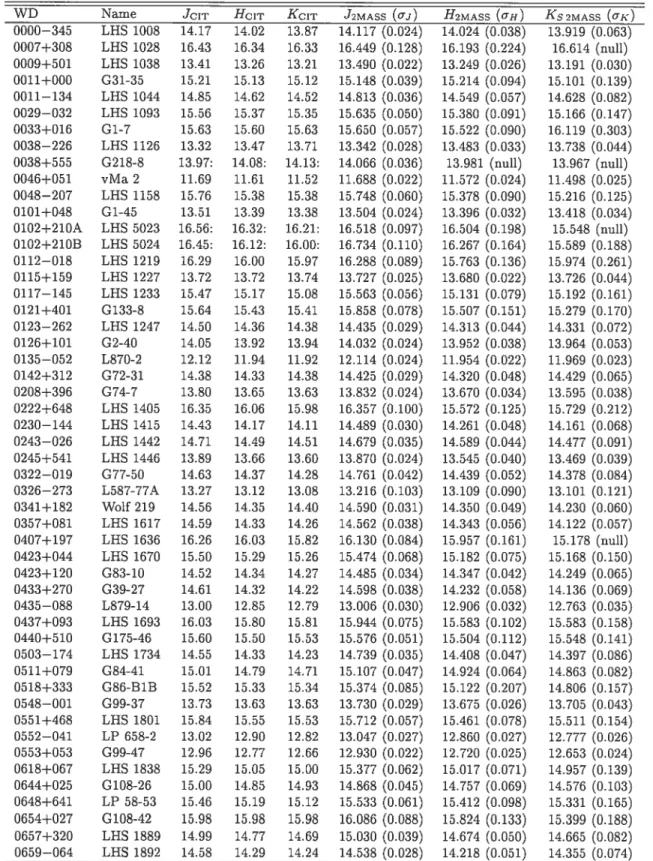
Figure 3.1 shows the differences in magnitudes between the infrared CIT and 2MASS photometric systems for the J, H, and K/Ks ifiters for the white dwarfs from Table 1. Note that the number of stars in each panel is different (159 in J, 157 in H, and 143 in Ks) since some stars have not been formally detected in one or more bands, and only lower limits are available. The size of the error bars in Figure 3.1 correspond to the combined quadratic uncertainties of both data sets, u = (uMASS +IT)’2• For both measurements to
be compatible, the error bar must touch the horizontal dashed line in each panel of Figure 3.1, which represents the mean magnitude difference between both data sets, as determined below.
CHAPITRE 3. WHITE DWARFS FROM 2MASS AND THE $PITZER TELESCOPE 14
We present in Table 2 a statistical comparison of both data sets for ail three hands. The flrst three unes correspond to the full data set while the last three unes are restricted to 2MASS magnitudes that satisfy the level 1 requirements. The second column indicates the number of stars used for the comparison (to be included. the 2MASS magnitude must have a measurement error). The third and fourth columns represent respectively the mean and the standard deviation of the magnitude differences for each band. These mean values thus correspond to the zero point offsets between both photometric systems, and we therefore adopt the following transformation based on the most accurate subsample (level 1): JCIT =
J2MASS — 0.0083, HCIT = H2MASS + 0.0094 and KCJT = K5 2MASS + 0.0133. We note that the offsets are typically five times smaller than the average 2MA$S uncertainties given in the flfth column of Table 2, (J2MASS) and these could as well be considered as zero for most
practical purposes. We also note that since the effective wavelength of the 2MASS K8 filter (2.169 im) is slightly shorter than that of the CIT K filter (2.216 jtm), the observed flux should be larger at K8 than at K, and a larger positive offset is thus expected for this baud, as is indeed observed in Table 2.
If the uncertainties of both data sets have been properly evaluated, the average combined quadratic uncertainties, (u) (last column of Table 2), should be at least as large as the standard deviations of the magnitude differences (fourth column of Table 2). This is certainly the case for the level 1 subsample, a result that conflrms the reliability of the 2MA$S level 1 photometry. For the complete sample, however, the (u) values are slightly below the standard deviations. If we assume that the CIT photometric uncertainties have been properly estimated, which is supported in 3RL97 and BLRO1 by the successful fits with white dwarf models, the 2IvIASS uncertainties might be slightly underestimated in the case of faint cool white dwarfs near the survey limit. Another way of interpreting these results is to note that in Figure 3.1, the magnitudes are not compatible within the lu combined uncertainties for 34.6%, 30.6%, and 35.0% of the stars in the complete sample at the J, H and K hands, respectively. These correspond to the objects whose error bars do not cross the horizontal dashed unes. This occurs for level 1 and fainter objects as well. At a 3u level, these numbers drop to 0.6%, 1.9% and 4.2%, respectively, which suggest that there are infrequent but large discrepancies at K8.
In Figure 3.2, we compare (J — H, H— K/Ks) two-color diagrams for various data sets. In the upper panels, we compare the two-color diagrams for the 143 stars in common in both the CIT and the 2MASS samples that have been detected by 2MASS in ail three bands. The 2MAS$ coiors appear much more scattered than the CIT colors, and this simply reftects the larger uncertainties of the former data set. Indeed, if we restrict the sample to the 49 objects that satisfy the level 1 requirements, the scatter of the 2MA$$ diagram is greatly reduced, as shown in the bottom panels of Figure 3.2. For this restricted sample, both CIT and 2MASS data appear to have a similar scatter, which is a confirmation of the comparable mean uncertainties. Since the 2MASS photometry has been used to infer the presence of unresolved white dwarf and low mass main sequence binaries, one needs to be cautious when interpreting data sets that include objects below the level 1 requirements.
For instance, we indicated by open circles in Figures 3.1 and 3.2 ten objects whose optical BVRI and infrared JHK photometry on the CIT system has been successfully fitted with single white dwarf models by 3RL97 and BLRO1. They cover a range in 2MA$S J magnitudes from 13.5 to 17. Our best fits for these stars are dispiayed in Figure 3.3. The fitting technique used here is described at length in BRL9Z. Briefiy, the magnitudes on the CIT system in Table 1 are first transformed onto the Johnson-Glass system using the transformation equations given by Leggett (1992). These magnitudes are then converted into observed fluxes using the method described by Holberg & Bergeron (2006) for photon counting devices but using the transmission functions taken from Besseli (1990) for the BVRI filters on the Johnson-Cousins photometric system, and from Bessell Brett (198$) for the JHK filters on the Johnson Glass system. The resulting energy distributions are then compared with those predicted from our model atmosphere calculations, properly averaged over the same filter bandpasses. The hydrogen- and helium-rich model atmospheres used in our analysis are similar to those described in BLRO1 and references therein, except that for the hydrogen-rich models we are now making use of the more recent H2-H2 collision-induced opacity calculations of Borysow et al. (2001) and the Hummer-Mihalas occupation probability formalisrn for ail species in the plasma. We find that the differences in the fitted parameters are small compared to those derived by BLRO1, however.
CHAPITRE 3. WHITE DWARFS FROM 2MASS AND THE SPITZER TELESCOPE 16
The effective temperature Teff, the solid angle ir(R/D)2 (with R the radius of the star and D its distance from Earth), and the atmospheric composition (H- or He-rich) are oh tained through a
x2
minimization technique, where thex2
value is taken as the sum over ail bandpasses of the difference between observed and predicted fluxes, properly weighted by observational uncertainties. The trigonometric parallax measurement, when available, is used to constrain the surface gravity through the mass-radius relation for white dwarfs, otherwise a value of log g = 8.0 is assumed. In Figure 3.3, the observed BVRIJHK fluxes are shownas error bars together with the monochromatic model fluxes (for clarity, we do not show the average model fluxes at each bandpass). The derived atmospheric parameters are given in each panel. As can be seen, the energy distributions for ail objects can be successfully reproduced by assuming a single star model.
Also reproduced in Figure 3.3 are the 2MASS magnitudes converted into fluxes using the 2MASS zero points of Holberg Bergeron (2006). We note that for 9 of the 10 objects, at least one of the fluxes at J, H, or K is flot compatible with the predicted fluxes within the
lu 2MA$S uncertainties. One exception is 0029—032, discussed later in
§
3.4. for which the model spectrum matches the 2MASS photometry even better than the CIT photometry. We thus conclude this section by stating that while the 2MASS photometry is generally reliable, one should expect occasional discrepancies. In particular, the detailed fits (not shown here) to the energy distributions using the 2MASS photometry are of good quality for most stars in our sample.3.4
WHITE DWARFS AND LOW
MASS MAIN SEQUENCE
BINARIES FROM 2MASS
3.4.1 The Wachter et al. Analysis
One of the most immediate applications to a large data set of white dwarf NIR photometry such as 2MASS is to seek infrared excesses due to cooler companions that are otherwise invisible in the optical. Wachter et al. (2003) used a sample of 759 white dwarfs from the catalog of McCook r Sion (1999) and identifled as many as 95 binary candidates and 15
tentative binary candidates based on the analysis of a (J — H, H — K3) two-color diagram built from 2MASS photometry. They extracted JHK3 magnitudes from the 2MASS second incremental data release. Their binary candidates were selected from the color criterion (J — H) > 0.4, defined by the dashed horizontal unes in our Figure 3.2, while their 15 tentative binary candidates satisfy the criterion 0.2 < (H— K3) <0.5 and 0.1 < (J—H) <0.4, defined by the dotted rectangles in Figure 3.2. In the following, we use the 2MASS final data release to recover more precise and slightly different observed JHK3 magnitudes than those reported by Wachter et al.
Using the same color criteria to study the 2MASS sample of presumably single cool white dwarfs presented in
§
3.3, we find in the upper-right panel of Figure 3.2 several binary and tentative binary candidates in both regions defined by Wachter et al. (2003). A comparison with the CIT pliotometry, however, reveals that this resuit can be readily explained in terms of the larger uncertainties of the 2MASS photometry since both regions are located 1 — 2u away from the region occupied by single white dwarfs near the center of the figure. We find that 3.5% and 8.4% of our sample observed by 2MASS contaminate the binary candidate and tentative binary candidate regions, respectively. By comparison, we find that at least 12.5% of the white dwarfs in the complete sample of 759 objects of Wachter et al. are located in the binary candidate region5. This indicates that the color criterion defined to identify companions is certainly appropriate, but also that the contamination from faint objects with large llncertainties near the 2MASS detection threshold may be significant. Furthermore, our large contamination of the tentative binary candidate region suggests that this criterion is not stringent enough, and that the corresponding subsample identified by Wachter et al. (2003, Table 2) is mostly composed of single white dwarfs.These conclusions are supported by the fact that one of the objects selected in the list of binary candidates (0102+210B) and four objects in the list of tentative binary candidates (0029—032, 0518±333, 0816+387, and 1247+550)6 are ail part of the single white dwarfsample described in
§
3.3 and whose fits are displayed in Figure 3.3. As can be seen, the CIT pho5The actual percentage may be larger depending on how many faint objects with a partial detection are
removed from the sample.
6We also found that the 2MASS identification of 0145—174 by Wachter et al. is erroneous; the actual star is much fainter and flot recovered in the 2MASS PSC.
CHAPITRE 3. WHITE DWARFS FROM 2MASS AND THE $PITZER TELESCOPE 1$
tometry for ail objects is well reproduced with single star model atmospheres. For 0029—032, our fit is even better using the 2MASS photometry than the CIT data. For the other stars, the 2MASS energy distributions appear flatter than those inferred from the CIT photometry or the model spectra, a result that could be interpreted as a flux excess in the K hand.
3.4.2
The Wellhouse et al.
AnalysisUsing a similar approach but with slightly different criteria, Wellhouse et al. (2005) sought companions to 51 magnetic white dwarfs as candidates for potential pre-cataclysmic variables. They proposed to spiit the (J — H, H — K8) two-color diagram into four regions delirniting (I) single white dwarfs, (II) main sequence binary candidates, (III) white dwarfs with very low mass companions, and (IV) objects that may be contaminated by circu;nstellar material. These representative regions are divided according to previous findings by Wachter et al. (2003) as well as theoretical color simulations. While they did not find any convincing binary candidates (region II), Wellhouse et al. identified six objects with a possible very low mass companion (region III) and four white dwarf candidates with an excess at K8 (region IV), which they interpreted as a signature of undetected planetary nebulae. This represents a total of 28.6% of their sample with formai uncertainties with a possible companion or a disk.
The four regions defined by Wellhouse et al. (2005) are reproduced here in the (J—H, H— K8) two-color diagram shown in figure 3.4, together with our common sample of CIT and 2MASS data composed of presumably single white dwarfs. From this figure, we flnd that 21% of the white dwarfs in the 2MASS data set would be considered possible candidates for a companion or a disk, while the CIT data show little evidence for such infrared excesses. This strongly suggests that the sample of magnetic white dwarfs studied by Wellhouse et al. could be entirely consistent with single stars. In addition, we note that among the six objects located in region III of Figure 1 from Wellhouse et al. are some of the most intrinsically peculiar white dwarfs7: LHS 2229 (1008+290) has been reported by Schmidt et al. (1999) and it has the strongest C2-like features ever observed, LP 790-29 (1036—204) is the strongest magnetic DQ known, and CD 229 (2010±310) shows strong unidentified absorption features in the optical
7Also, 2201—228 in that sample is probably not magnetic according to S. Jordan (2005, private communi cation).
(Wesemael et al. 1993, Fig. 19). Therefore, region III seems to 5e populated with some ofthe most peculiar white dwarfs for which there is no reason to expect their NIR colors to overlap with those of normal white dwarfs. Similarly, if we restrict our analysis to the more accurate CIT data, there are three white dwarfs located in region III of our Figure 3.4. Two of these identified in the figure are also peculiar: G240-72 (1748+708) shows a deep yellow sag in the 4400-6300
À
region (Wesemael et al. 1993, Fig. 19), and LP 701—29 (2251—070) is a heavily blanketed DZ star (Wesemael et al. 1993, Fig. 11).We also note that ail four objects in region IV of Wellhouse et al. (2005, Fig. 1) are very faint stars with 2MASS Ks uncertainties in the range 0.16-0.27. As seen in our Figure 3.4, we do expect single white dwarfs with large uncertainties to populate this particular region as well. Hence the location of the four objects identified by Wellhouse et al. in this particular region of the (J—H, H—K) two-color diagram is most naturally explained in terms of the low quality of the 2MASS data for these objects rather than the presence of planetary nebulae. We thus conclude that the identification of NIR excesses in the 2MASS PSC database requires more conservative criteria allowing for larger uncertainties in the photometric measurements below the level 1 requirements, or more accurate methods such as that presented in the following section.
3.4.3
The Synthetic Flux Method
Another technique for identifying binary candidates is to compare observed 2MA$S fluxes directly with those predicted from model atmospheres (see. e.g., Holberg Magargal 2005; Holberg & Bergeron 2006). Effective temperatures and surface gravities are first obtained using the spectroscopic method developed by Bergeron et al. (1992) where high signal-to-noise spectroscopic observations of the hydrogen Balmer unes are fitted with synthetic models. The model flux is then normalized to the observed V magnitude to predict the observed fluxes at J, H, and K using the 2MASS filter passbands from Cohen et al. (2003) and the zero points from Holberg & Bergeron (2006). Thus, only objects with known atmospheric parameters and V magnitudes can 5e used with this method. In what follows, we rely on the fitting technique and NLTE model atmospheres for DA stars described in Liebert et al. (2005) and references
CHAPITRE 3. WHITE DWARFS FROM 2MASS AND THE SPITZER TELESCOPE 20
therein.
To illustrate the method, we selected ail DA stars from Wachter et al. (2003) for which we had an optical spectrum and a published V magnitude. In Table 3, we present our sample that includes 42 binary candidates and S tentative binary candidates from Tables 1 and 2 of Wachter et al. (2003), respectively8. For each object, we give the atmospheric parameters (Teff and logg), the published V magnitude, and the predicted and observed 2MASS magnitudes at J, H, and K3. In some cases, the optical spectrum was signiflcantly contaminated by the unresolved companion, and the uncertainties on the derived parameters are correspondingly larger; these are indicated by colons in Table 3.
For most objects, a significant NIR excess is observed, with the 2MASS data being typically ‘-.2 magnitudes brighter than the values predicted from the model fits. In Figure 3.5, we present typical results for ten objects selected from Table 3. Here we show the observed 2MASS fluxes together with the predicted monochromatic fluxes calculated at the atmospheric parameters given in each panel. For 0023+388, 0034—211, 0131—163, and 0145—257, the companion can be unambiguously detected since the 2MASS fluxes are about a factor of 10 to 100 larger than the predicted fluxes. For 0145—221, only a mild NIR excess is observed and this object has indeed been identified as a WD+dL6/7 by Farihi et al. (2005) and Dobbie et al. (2005). Two of the tentative binary candidates, 0710+741 and 2257+162, do indeed show a significant excess consistent with a very low mass companion. Farihi et al. (2005) have actually conflrmed that 0710+741 is a WD+dM7. However, for 1434+289, 1639+153, and 2336—187, which are tentative binary candidates in Wachter et al. (2003), we do not observe any significant NIR excess and these objects are thus consistent with being single white dwarfs.
With the exception of these last three objects, the infrared excesses observed in Table 3 are consistent with iinresolved low-mass main sequence M dwarfs physically associated with the white dwarfs (Farihi et al. 2006). Photometric observations of single M dwarfs by Leggett et al. (1996) show that the (J—V) color index is in the range from ‘- 2 to 4, while single cool white dwarfs are expected to be in the range from —1 to 1. This explains why tlie contribution
8Note that the 2MASS identification for 40 En B (0413+077) by Wachter et al. is erroneous. With two
objects within 2”, they picked what is probably the M dwarf 40 En C instead of 40 En B itself. Thus, whule
this is stiil technically a WD+dM binary, both objects are barely resolved in 2MASS and we do not include them in our sample.
of the M dwarf can be dominant in the NIR but negligible in the optical. Many of the 44 remaining binary candidates in Table 3 have been discussed in the literature. For instance,
Farihiet al. (2005) and Farihi et al. (2006, with HST) observed 28 candidates from this list and were able to resolve the red dwarf companion(s) for 17 objects. The NIR excesses were also conflrmed by Farihi et al. (2005); Farihi et al. (2006) using JHK photometric observations for the 11 remaining unresolved objects. The presence of a companion for 9 additional objects in Table 3 has been discussed at various degrees in the literature, while for the 7 remaining binary candidates (0812+478, 0915+201, 1037+512, 1108+325, 1339+346, 1610+383, and 2257+162), we conflrm through the synthetic flux method a strong NIR excess consistent with the presence of low mass main-sequence companions.
We have seen that for a brown dwarf companion, the flux excess is not as important as for M dwarfs. In the case of the dL6/7 dwarf coinpanion to 0145—221, the flux excess at K5 is stili significant at the 12 level, however, according to Table 3. There is only one known example of a companion with a possible later spectral type, the brown dwarf companion to 0137—349, discovered from radial velocity measurements by Maxted et al. (2006), who also report a small excess at K5 from 2MASS PSC data. Burleigh et al. (2006) aso present a near-IR spectrum that conflrms the slight K-band excess they attribute to a dL8 companion. We analyzed the 2MASS photometry of this object with the method described in this section, and assumed the effective temperature and surface gravity from Maxted et al. (2006). We were able to match very well the predicted and observed 2MASS J magnitude within the uncertainties, and also identifled a flux excess at K5 at the 2.49 level, which is barely significant, but stili consistent with the presense of a disk or a companion. Therefore, the 2MASS survey is able to identify bot brown dwarf companions, but it becomes more difficult to conflrm their presence for spectral types later than about dL7.
We end this section by asserting that methods based on comparisons of observed and predicted 2MASS fluxes (or magnitudes) represent an efficient way of identifying unresolved white dwarf and low-mass main sequence binaries down to late-type L dwarfs. Our analysis also reveals, however, that (J— H, H— Ks) two-color diagrams based on 2MAS$ data should be interpreted with caution, and that regions expected to contain unresolved binaries may be
CHAPITRE 3. WHITE DWARFS FROM 2MA$S AND TEE SPITZER TELESCOPE 22
contaminated with single white dwarfs, especially when data below the level 1 requirements are considered.
3.5
INFRARED PHOTOMETRY FROM SPITZER
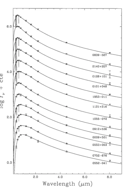
The Spitzer Space Tetescope lias been used to secure for the flrst time IRAC 4.5 and 8 ,um photometric data for relatively bright, nearby white dwarfs (see, e.g., Hansen et al. 2006). Que of the main interests of these surveys is to look for infrared flux excesses due to the presence of circumstellar disks since it is expected that the cool disk would dominate the MIR flux. It is however necessary as a flrst step to evaluate the reliability of the Spitzer data set and the ability of the mode! atmospheres to reproduce the MIR fluxes. In such an effort, Kilic et al. (20065) compared the $pitzer 4.5 and 8 im photometric data of 18 cool and bright white dwarfs with the predictions of model atmospheres. They found that the four hydrogen atmosphere white dwarfs with Teff 6000 K show a slight flux depression at 8 m, while one peculiar object, the so-called C2H star LHS 1126, suffers from a significant flux deflcit at both 4.5 and 8 im. For the warmer objects, the model fluxes seem to reproduce the SpitzeT data perfectly.
In this section, we reanalyze 14 objects from the sample of Kilic et al. (2006b) for which optical BVRI photometry and infrared JHK photometry on the CIT system are available (ail of these are already part of our cool white dwarf sample discussed in
§
3.3). In an approach similar to that described in§
3.3 (see Fig. 3.3), we determine the atmospheric parameters for each star by fltting simultaneously the average fluxes for the nine photometric bauds (BVRI, JHK/CIT, and $pitzer 4.5 and 8 jim). The synthetic fluxes in the MIR are obtained by integrating our model grid over the $pitzerIRAC spectral response curves while the observed fluxes are taken directly from Table 1 of Kilic et al. (20065). In contrast with the technique used by Kilic et al., we do not normalize the fluxes at any particular hand, but consider instead the solid angle r(R/D)2 a free parameter. Since our x2 value is taken as the sumover ah bauds of the difference between observed and model fluxes, properly weighted by the corresponding observational errors, our approach lias the advantage of allowing for the full photometric uncertainties in the fltting procedure. Furthermore, instead of assuming log g =
8.0 for ail objects, we constrain the log g value from the trigonometric parallax measurernents, as described above.
In Figure 3.6, we present our best fits on a logarithmic scale to the observed BVRI, JHK (CIT), and Spitzer photometry with the model average fluxes described above. We also plot the monochromatic fluxes for clarity; the case of LHS 1126 is discussed separately below. Another peculiar object, G240-72 (1748+708) already discussed near the end of
§
3.4.2, shows a deep unidentifled absorption in the optical ta yellow sag) and no satisfactory fit can 5e achieved for this star and it is thus left out of our analysis. For Ross 627 (1121+216), the 8 jim flux is not shown in Figure 3.6 since Kilic et al. (20065) provides oniy an upper limit due to a possible contamination from a nearby star. Our final sample thus includes 12 stars with 23 Spitzer 4.5 and 8 im flux measurements. For all cases shown in Figure 3.6, the Spitzer fluxes are well reproduced by the synthetic models. To further strengthen this conclusion, we plot in Figure 3.7 the ratio of the observed to model fluxes at 4.5 and 8 im as a function of the derived effective temperature for the 12 objects. The figure conflrms the agreement between the observed Spitzer and model fluxes at ail temperatures. In particular, we do not observe any significant flux deficit at low effective temperatures as suggested by Kilic et al. (20065). There are only 2 observations out of 23 for which the flux deficit is significant at the 1 level, and both are in the 8 im baud. It thus seems premature to conclude from these results that there is any discrepancy between the observations and the predictions of model atmospheres with pure hydrogen compositions.We mention in this context that the second coolest object in Figure 3.7 is the DA star BPM 4729 (0752—676) for which we obtain a perfect fit. This star has been studied extensively by BLRO1, and more recently by Kowalski Saumon (2006) using improved L profiles that inciude broadening by molecuiar hydrogen, and both atmospheric parameter determinations agree at the lu level under the assumption of pure hydrogen compositions. Hence for this well studied normal cool DA star, independent model atmospheres yield consistent atmospheric parameters that both match the observational data. In contrast, the two objects -LHS 1038
(0009+501) and G99-47 (0553+053) with the small 8 im flux discrepancies (bottom panel of Fig. 3.7) are magnetic white dwarfs. Both objects show lu discrepancies at J and also at 3
CHAPITRE 3. WHITE DWARFS FROM 2MÀSS AND THE SPIIZER TELESCOPE 24
for G99-47. While this suggests that the inclusion of a magnetic fleld in the model atmosphere calculations could improve the fit, we believe that the discrepancies observed here are oniy barely significant and not systematic enough to make formai conclusions. Therefore, we argue that the resuits presented in this section demonstrate the reliability of both the $pitzerIRAC photometry and our model atmosphere grid up to 8 im for studying cool white dwarfs. The consistency between models and data is critical for surveys seeking MIR infrared excesses from circumstellar disks. Our resuits indicate that the comparison of$pitzerfluxes with theoretical predictions could identify such MIR excesses with relatively high precision.
In an attempt to identify the nature of the discrepancy between our conclusions and those reached by Kilic et al. (2006b), we have performed the same anaiysis as above but with the 2MASS JHK8 magnitudes used by Kilic et al. (instead of the CIT magnitudes used in this analysis). We have also tried to normalize our solutions at V, as done by Kilic et al. In all of our experiments, the results differ only slightly from those reported here, and our main conclusions thus remain the same. We are therefore unable to explain the differences between both studies. We can only emphasize that the analysis of Spitzer photometric data appears to 5e sensitive to the details of the fltting procedure.
Another white dwarf analyzed by Kihc et al. (2006b) is LHS 1126 (0038—226) whose energy distribution is characterized by a strong infrared flux deflciency at JHK interpreted by Bergeron et al. (1994) in terms of collision-induced absorption (CIA) by molecular hydrogen due to collisions with helillm in a mixed hydrogen and helium atmosphere with N(H)/N(He)
-0.01. We do conflrm here the results shown in Figure 4 of Kilic et al. (20065) where the Spitzer fluxes are signiflcantly depressed with respect to the predictions of model atmospheres with mixed compositions. The main reason for this discrepancy is that the CIA opacity predicts a maximum absorption near the H2 fundamental vibration frequency at - 2.4jim, while the
Spitzerfluxes are more consistent with a featureless energy distribution from 1 to 8 tm. This problem is surprisingly similar to that encountered in the so-called ultra-cool white dwarfs, and in particular in the case of LHS 3250 for which the H2-H2 and H2-He CIA opacities predict absorption bands that are simply not observed in spectroscopy (Bergeron & Leggett 2002). These results may indicate that the collision-induced opacity calculations need to 5e
improved at the high densities encountered in cool white dwarf atmospheres.
3.6
CANDIDATE WHITE DWARFS WITH CIRCUMSTEL
LAR DISKS
The synthetic flux method based on a comparison of predicted and observed 2MASS fluxes (or magnitudes) was shown to be an efficient technique for detecting NIR excesses from unresolved companions
(
3.4). However, the NIR excess in the JHKs hands expected from cool circumstellar disks or planets surrounding white dwarf stars can 5e extremely small if the flux is dominated by the white dwarfin this particular wavelength range. In this section, we use the results of the ongoing spectroscopic survey of Gianninas et al. (2006) together with the 2MAS$ PSC to search for massive disks resulting from the merger of two white dwarfs, as predicted by Livio et al. (2005). In addition to the synthetic flux rnethod described above, we also compare the observed and predicted (J— H) and (J— K) color indices since this method lias the advantage of Seing independent of the normalization at V, which allows us to consider also objects with no published V magnitudes. $ince circumstellar disks are expected to 5e much brighter at K than in the other bands, we expect their color indices to be very different from those of single white dwarfs, and such objects should easily stand out in our analysis.
As discussed in the Introduction, white dwarfs resulting from mergers are expected to be found in the high-mass tail of the mass distribution. We thus selected all DA stars from the survey of Gianninas et al. (2006) with spectroscopic masses above 0.8 M0 that were formally detected by 2MASS in at least two bauds (usually the J and H bauds), for a total of 57 objects. In Table 4, we provide the effective temperature, the spectroscopic mass, the V magnitude (when available), as well as the predicted and observed 2MASS JHK8 magnitudes for each object in our sample. The atmospheric pararneters (I and 10g g) are obtained from fits to the Balmer lines using the NLTE model grid described in
§
3.4, and the log g values are converted into mass using the evolutionary models of Wood (1995) with carbon-core compositions and thick hydrogen layers. The predicted fluxes are obtained from the synthetic flux method andCHAPITRE 3. WHITE DWARF$ FROM 2MASS AND THE SPITZER TELESCOPE 26
are thus orfly given for objects with measured V magnitudes.
Five white dwarfs in Table 4 (0429+176, 0950+139, 105$—129, 1120+439, and 1711+668) show a large NIR ftux excess that is not attributable to a circumstellar disk. The predicted spectra for these stars are shown in Figure 3.8 together with the observed 2MASS fluxes. We discuss each object in turn.
HZ 9 (01,29+176) — This object is a WD+dM binary (Lanning et al. 1981) in common with the sample discussed in
§
3.4.FG 0950+ 139 — This star is in common with the sample discussed in
§
3.4. The white dwarf is surrounded by a planetary nebulae (Ellis et al. 1984) and its optical spectrum exhibits emission hues (Liebert et al. 1989). According to Fulbright et al. (1993), the low-density gas ernission and the infrared excess are best explained by the presence of a low-mass companion. FG 1058—129, PG 1120+1,39 - These two objects show a mild and unexplained infrared ex cess. In both cases, the only V magnitudes available are multichannel data from the Palomar Green survey (Green et al. 1986). Since the observed energy slopes measured by color indices are in perfect agreement with those predicted by the models (see below), it is very likely that the V magnitudes for these stars are simply erroneous. We note that Green et al. (2000) also determined a 1-sigma significant excess at J for PC 1120+439.RE J1711+664 (1711+668) — This white dwarf is a barely resolved visual pair (Finley et al. 1997). The predicted NIR flux from this white dwarf is too low to be detected by 2MASS. Thus only the dM star 2” away from the white dwarf is detected in the PSC.
We exclude from our analysis the three objects with known companions, but we keep PG 105$—129 and PG 1120+439.
We compare in Figure 3.9 the observed and predicted (J—H) and (H— K) color indices as a function of H and K, respectively, for the remaining 54 white dwarfs in our sample. An examination of these results indicate that all stars are consistent with the predicted white dwarf colors within 3a uncertainties, both above and below the level 1 requirements. Two glaring exceptions are G1-7 (0033±016) and CBS 413 (1554+322), wliich are among the faintest objects in the bottom panel of Figure 3.9 (labeled 1 and 2, respectively). For G1-7, however, the color indices derived from the CIT photometry given in Table 1 are in excellent
agreement with those predicted by the models. Also, CBS 413 bas not been detected at H but it is unexpectedly bright at K8! Since this object has no published V magnitude, it is flot clear whether the J detection is indeed from the white dwarf. and thus whether the color excess at K8 is even real. Therefore, we conclude from the resuits shown in Figure 3.9 that there is no strong evidence for H or K8 excesses in this sample of massive white dwarfs, and for the presence of massive circumstellar disks around them.
For comparison, we also reproduce in Figure 3.9 the location of three white dwarfs with previously identifled circumstellar disks: G29-38 (2326+049), GD 362 (1729+371) and CD 56 (0408—041). The atmospheric parameters for all three stars have been determined using our own spectroscopic observations, and the predicted 2MASS color indices have been estimated from the same method as above. For the metal-rich DAZ star CD 362, we use the more accurate atmospheric parameters of Gianninas et al. (2004) who took into account the presence of heavy elements in their model atrnosphere calculations. Only GD 362 in our sample is a massive white dwarf with M = 1.24 M0. while we obtain M = 0.70 and 0.60 M0 for
G29-38 and GD 56, respectively. The disk around G29-G29-38 vas the flrst discovered and studied extensively in the MIR (Reach et al. 2005). The object is clearly identifiable in Figure 3.9
with(JKS)2MASS(JKS)pred 0.52±0.04, a’ l2uresult. The second object, GD 362, is
a massive DAZ star for which Becklin et al. (2005) reported the discovery of an important flux excess at L’ (3.76 m) and N’ (11.3 km). Kilic et al. (2005) obtained a near infrared spectrum in the 0.8 — 2.5 zm range but found only a mild flux excess at K. Both studies concluded that the presence of a dust disk could account for the observations. Given that GD 362 is particularly faint (V = 16.3), only lower limits at H and K3 are available in the 2MASS P$C.
Instead, we use in Figure 3.9 the JHK3 magnitudes measured by Beckiin et al. (2005). With these measurements, GD 362 exhibits a color excessOf(J—K3)obs—(JKS)pred 0.22±0.04, a 5g result. Unfortunately, this photometric accuracy is only achieved in the 2MASS sample for J brighter than 14.1, and a color excess of the magnitude found in GD 362 cannot be easily uncovered in the majority of white dwarfs detected by 2MASS. For GD 56. Kilic et al. (2006a) reported a NIR excess in both the 2MASS data and in their own infrared spectroscopic observations. Unlike the two previous objects, GD 56 lacks the MIR observations that could