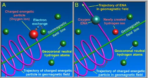
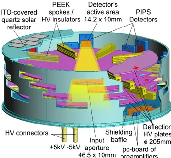
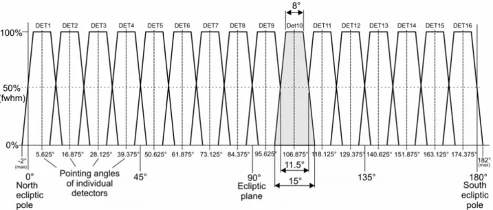
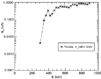
The NUADU experiment on TC-2 and the first Energetic Neutral Atom (ENA) images recorded by this instrument
26
0
0
Texte intégral
Figure
+7


Documents relatifs