DYNAMIC PREDICTION OF TRAFFIC CONDITIONS USING STREAMING DATA AND BAYESIAN APPROACH
MOHAMMAD KIANPOUR
DÉPARTEMENT DES GÉNIES CIVIL, GÉOLOGIQUE ET DES MINES ÉCOLE POLYTECHNIQUE DE MONTRÉAL
MÉMOIRE PRÉSENTÉ EN VUE DE L’OBTENTION DU DIPLÔME DE MAÎTRISE ÈS SCIENCES APPLIQUÉES
(GÉNIE CIVIL) JANVIER 2017
c
ÉCOLE POLYTECHNIQUE DE MONTRÉAL
Ce mémoire intitulé :
DYNAMIC PREDICTION OF TRAFFIC CONDITIONS USING STREAMING DATA AND BAYESIAN APPROACH
présenté par : KIANPOUR Mohammad
en vue de l’obtention du diplôme de : Maîtrise ès sciences appliquées a été dûment accepté par le jury d’examen constitué de :
M. TRÉPANIER Martin, Ph. D., président
M. FAROOQ Bilal, Ph. D., membre et directeur de recherche M. PATTERSON Zachary, Ph. D., membre
DEDICATION
To my wife. That without her support I could not continue. And to my older son, that without his understanding I had stopped.. . .
ACKNOWLEDGEMENTS
I am very grateful to my supervisor, Prof. Bilal Farooq, whose encouragement, guidance, hours of assistance, sound advices, and dedication immeasurably improved this thesis, and indeed were indispensable to its completion. I am thankful for these thoughtful and insightful comments to ensure that a quality document will result from this endeavor.
I really appreciate the valuable help of Prof. Catherine Morency and the City of Montréal for providing me with the data. Also, I must thank Dr. Anae Sobhani and Mr. Hamzeh Alizadeh, PhD candidate, for the time that they spent on reading this thesis and their comments for better writing the document.
RÉSUMÉ
La diffusion des données peut être définie par son volume remarquable, la génération de vitesse, la richesse de l’information et la diversité de l’information. Aujourd’hui, de grandes quantités de données, produites par de nombreuses sources nouvelles, peuvent être classées dans ce type de données. Des domaines tels que le transport et l’ingénierie du trafic peuvent bénéficier de ces ensembles de données. L’utilisation de diffusion de données pour créer de nouvelles méthodes de modélisation des comportements de déplacement peut être utile de trois manières. Tout d’abord, cela peut réduire le temps requis et le coût de collecte de données suffisantes avec les méthodes conventionnelles. Deuxièmement, cela peut augmenter le niveau de précision des modèles proposés et les simulations mises en œuvre. De plus la diffusion de données peut réduire la dépendance à l’égard des données traditionnelles. La prédiction des conditions de circulation a des effets notables sur la diminution des ef-fets nocifs de la congestion dans un réseau urbain. Dans cette thèse, nous définissons une approche pour l’utilisation de la diffusion des données provenant de diverses sources dispo-nibles de façon ubiquitaire, par ex. Les traces de GPS (Global Positioning System), la caméra de trafic, l’approvisionnement de foule, etc. La diffusion de données nous donne la possibilité d’utiliser plus d’informations avec les sources de données traditionnelles pour développer des modèles de transport urbain. Par conséquent, nous élaborons un cadre qui utilise des données en continu pour prédire les conditions de circulation à court terme au niveau du lien dans un réseau urbain. L’approche bayésienne qui définit la probabilité d’un événement basé sur d’autres événements expérimentés a été mise en œuvre pour mettre à jour la probabilité de conditions de circulation possibles. En utilisant l’approche bayésienne qui exploite la diffusion de données en continu, nous créons un nouveau type de modèle de prédiction du trafic dans cette étude.
Nous élaborons un modèle de prévision qui utilise les connaissances existantes sur les condi-tions du trafic urbain et les données en continu fournies en tant que nouvelles sources non traditionnelles. Les conditions de circulation sont simulées par un modèle antérieur. En dé-veloppant l’approche bayésienne pour prédire la probabilité d’un état, en utilisant à la fois la simulation des conditions de circulation et les mesures provenant des sources de données en continu, nous considérons la probabilité de notre connaissance préalable des conditions de circulation, la probabilité des mesures et le modèle conditionnel pour chaque état possible des conditions de circulation dans le réseau urbain.
La probabilité d’un état basé sur les données de diffusion disponibles est définie en multi-pliant la probabilité de l’état défini par le modèle précédent par le rapport de la probabilité
définie par le modèle conditionnel sur la probabilité des mesures. Nous définissons la liaison de réseau d’état par liaison. Le résultat de la méthode proposée est l’état le plus probable du système en considérant les données de diffusion disponibles à chaque temps. Par conséquent, nous sommes en mesure de recommander l’état le plus probable à chaque étape de temps ainsi que les paramètres de lien (vitesse, débit et densité).
L’approche proposée est appliquée à un cas réel pour démontrer la faisabilité de l’approche. Deux routes artérielles Nord-Sud vers le centre-ville de Montréal ont été considérées comme l’étude de cas. Les états probables du réseau urbain sont définis en simulant diverses condi-tions de circulation basées sur différents ensembles de temps de déplacement qui sont dis-ponibles à partir des données fournies par les véhicules flottants qui ont parcouru les routes choisies.
Les résultats démontrent que l’approche bayésienne proposée est capable de nous guider dans la définition de l’état le plus probable du réseau routier urbain. Cette approche peut amélio-rer les capacités de prévision des conditions à court terme du réseau routier urbain.
De plus, les prévisions de trafic à court terme, en tant que modèle de mise à jour, peuvent aider les opérateurs et les utilisateurs des réseaux routiers urbains à optimiser leurs décisions d’exploitation et d’utilisation de ces réseaux.
Mots-clés: Mise à jour bayésienne, diffusion de données, Prévision de flux de trafic,
ABSTRACT
Streaming data can be defined by its remarkable volume, generation of speed, richness of information, and diversity of information. Today, large volumes of data, produced by many new sources, can be classified as this type of data. Domains such as transportation and traffic engineering can benefit from these datasets. Using streaming data to create new methods of travel behaviour modelling can be helpful in three ways. First of all, it can reduce the required time and cost of collecting sufficient data from conventional methods. Secondly, it can increase the accuracy level of proposed models and implemented simulations. Finally, it can reduce dependency on traditional cross-sectional data.
Predicting traffic conditions has noticeable effects on decreasing the harmful impacts of con-gestion in an urban network. In this thesis, we define an approach for using streaming data coming from various ubiquitously available sources e.g. GPS (Global Positioning System) traces, traffic camera, crowdsourcing, etc. Streaming data provides us with the possibility of using more information along with traditional sources of data to develop urban transporta-tion models. Therefore, we propose a framework that uses streaming data for predicting short-term traffic conditions at link level in an urban network. The Bayesian approach that defines the probability of an event based on other experienced events has been implemented to update the probability of possible traffic conditions. By using the Bayesian approach that exploits streaming data, we create a new type of traffic prediction model in this study. We develop a prediction model that uses the existing knowledge of urban traffic conditions and streaming data provided as new non-traditional sources. The traffic conditions are sim-ulated by a prior model. In developing the Bayesian approach to predict the probability of a state, using both simulation of the traffic conditions and measurements coming from the source of streaming data, we consider the probability of our prior knowledge of traffic condi-tions, the probability of measurements, and the conditional model for each possible state of traffic conditions in the urban network.
The probability of a state based on the available streaming data is defined by multiplying the probability of the network state defined by the prior model by the ratio of the probabil-ity defined by the conditional model over the probabilprobabil-ity of measurements. We define the network state link by link. The output of the proposed method is the most probable state of the system considering available streaming data at each time-step. Therefore, we are able to recommend the most probable state at each time-step as well as link parameters (speed, flow, and density).
ap-proach. Two North-South arterial routes to Montréal downtown have been considered as the case study. The probable states of urban network are defined by simulating various traffic conditions based on different sets of travel times that are available from the data provided by floating vehicles that have traveled the chosen routes.
Results demonstrate that the proposed Bayesian approach is able to guide us for defining the most probable state of urban road network. This approach can improve capabilities of short-term conditions prediction of the urban road network.
Moreover, short-term traffic prediction results, as an updating model, can help operators and users of urban road networks to optimize their decisions for operating and using these networks.
LIST OF CONTENTS DEDICATION . . . iii ACKNOWLEDGEMENTS . . . iv RÉSUMÉ . . . v ABSTRACT . . . vii LIST OF CONTENTS . . . ix
LIST OF TABLES . . . xii
LIST OF FIGURES . . . xiii
LIST OF SYMBOLS AND ABBREVIATIONS . . . xv
LIST OF APPENDICES . . . xviii
CHAPTER 1 INTRODUCTION . . . 1
CHAPTER 2 LITERATURE REVIEW . . . 4
2.1 Short-term prediction of traffic flow . . . 4
2.1.1 Detection technologies . . . 4
2.1.2 Short-term traffic prediction methods . . . 5
2.2 Traffic modelling frameworks . . . 9
2.2.1 Cell transmission model (CTM) . . . 9
2.2.2 Cellular automata (CA) . . . 9
2.2.3 Queue-based simulations . . . 10
2.2.4 Car-following models . . . 10
2.2.5 Comparison between traffic modelling frameworks . . . 12
2.3 Contribution of this study . . . 14
CHAPTER 3 METHODOLOGY . . . 17
3.1 General framework . . . 17
3.2 Bayesian updating approach . . . 19
3.4 Prior car-following traffic model . . . 23
3.5 Traffic simulation and calibration tool . . . 24
3.5.1 Lane changing effects . . . 25
3.5.2 Volume entering into each link from upstream . . . 25
3.6 Link state definition using speed . . . 26
3.7 Link state definition using density . . . 26
3.8 Defining probability of measurements . . . 28
3.9 Measuring conditional model . . . 30
3.10 Effect of dependency between connected links . . . 31
3.11 Algorithms for implementing the proposed methodology . . . 33
CHAPTER 4 CASE STUDY, DATA AND DESCRIPTIVE ANALYSIS . . . 36
4.1 Case study . . . 36
4.1.1 Detailed characteristics of the chosen routes . . . 37
4.2 Data description . . . 38
4.2.1 GPS dataset . . . 39
4.2.2 Traffic volume dataset . . . 45
4.2.3 Travel time dataset . . . 45
4.3 Data analysis . . . 51
4.3.1 Analysis of available GPS data . . . 51
4.3.2 Analysis of available counted data . . . 52
4.3.3 Analysis of travel time data . . . 52
4.4 Simulating the possible states of traffic conditions . . . 55
CHAPTER 5 IMPLEMENTING THE PROPOSED METHOD, RESULTS AND DIS-CUSSION . . . 57
5.1 Implementing the proposed methodology . . . 57
5.2 General results and discussion . . . 58
5.3 Results for sample link . . . 59
CHAPTER 6 SENSITIVITY ANALYSIS . . . 64
6.1 Sensitivity of the results to sampling rate . . . 64
CHAPTER 7 VALIDATION . . . 68
CHAPTER 8 CONCLUSION . . . 73
8.1 Benefits . . . 74
CHAPTER 9 FUTURE STUDIES AND DIRECTIONS . . . 76 BIBLIOGRAPHY . . . 78 APPENDICES . . . 82
LIST OF TABLES
Table 2.1 Applied approaches in short-term prediction of traffic flow . . . 8
Table 2.2 Summary of comparison between four traffic modelling frameworks . 14 Table 4.1 Summary of links’ characteristic in the chosen routes . . . 38
Table 4.2 Travel time (sec) in Acadie-Parc -SB direction . . . 49
Table 4.3 Travel time (sec) in Acadie-Parc -NB direction . . . 49
Table 4.4 Travel time (sec) in St. Urbain (SB direction) . . . 50
Table 4.5 Travel time (sec) in St. Laurent (NB direction) . . . 50
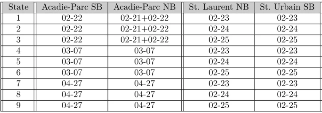
Table 4.6 Nine various inputs (series of travel times) for defining nine different possible states of the network of the case study . . . 51
Table 7.1 Result of validation . . . 68
Table 8.1 Limitation in implementing Poisson distribution . . . 75
Table A.1 Characteristic of the links in Acadie-Parc -SB direction . . . 82
Table A.2 Characteristic of the links in Acadie-Parc -NB direction . . . 83
Table A.3 Characteristic of the links in St. Urbain (SB direction) . . . 84
Table A.4 Characteristic of the links in St. Laurent (NB direction) . . . 85
Table B.1 Some rows of a recorded GPS traces as an example . . . 86
Table C.1 Start time of recording trajectories in Acadie-Parc -NB direction . . . 87
Table C.2 Start time of recording trajectories in Acadie-Parc -SB direction . . . 88
Table C.3 Start time of recording trajectories in St. Laurent-NB direction . . . 88
Table C.4 Start time of recording trajectories in St. Urbain-SB direction . . . . 88
Table D.1 Counted traffic data at intersections . . . 89
LIST OF FIGURES
Figure 2.1 Visual angle and the related factors . . . 12 Figure 2.2 Statement of contribution . . . 15 Figure 3.1 Conventional modelling framework without considering impacts of
re-cently experienced traffic conditions, based on Furnish and Wignall (2009) . . . 17 Figure 3.2 Improved network modelling framework using a Bayesian updating
fra-mework and user-centric streaming data for considering the impacts of recently experienced traffic conditions . . . 18 Figure 3.3 Defining the probability of a network state as prior knowledge
consi-dering available measurements using Bayesian framework . . . 20 Figure 3.4 Flow diagram describing the steps and processes required for defining
the most probable state of urban network at time t . . . . 21 Figure 3.5 Modelling the urban road network (a) at its two elements : Links (b)
and intersections (c) . . . 24 Figure 3.6 The steps used in the process of simulating possible states of traffic
conditions by SUMO and calibrating by SA method . . . 25 Figure 3.7 Link state at three times tji0 (a), t0ji (b), and t (c) and the volume
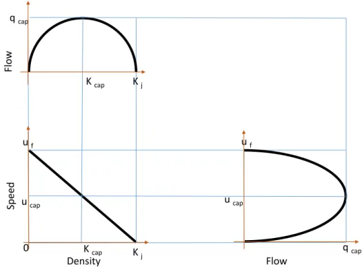
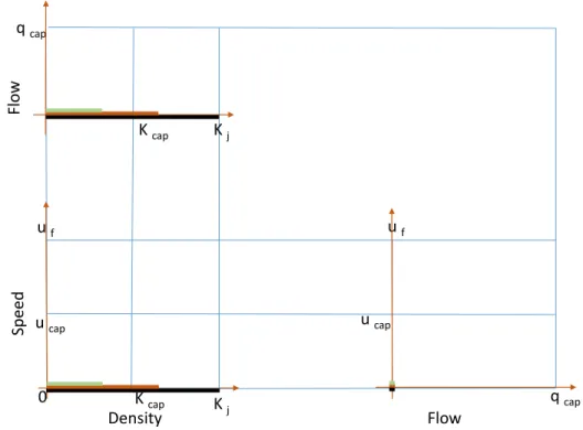
entering into each link between t0ji and tji0 (a) and t0ji and t (c) . . . . 27 Figure 3.8 Fundamental diagram when the value of speed is non-zero. . . 28 Figure 3.9 Fundamental diagram when the value of speed is zero. . . 29 Figure 3.10 A simple demonstration of link i1 connected to the other links through
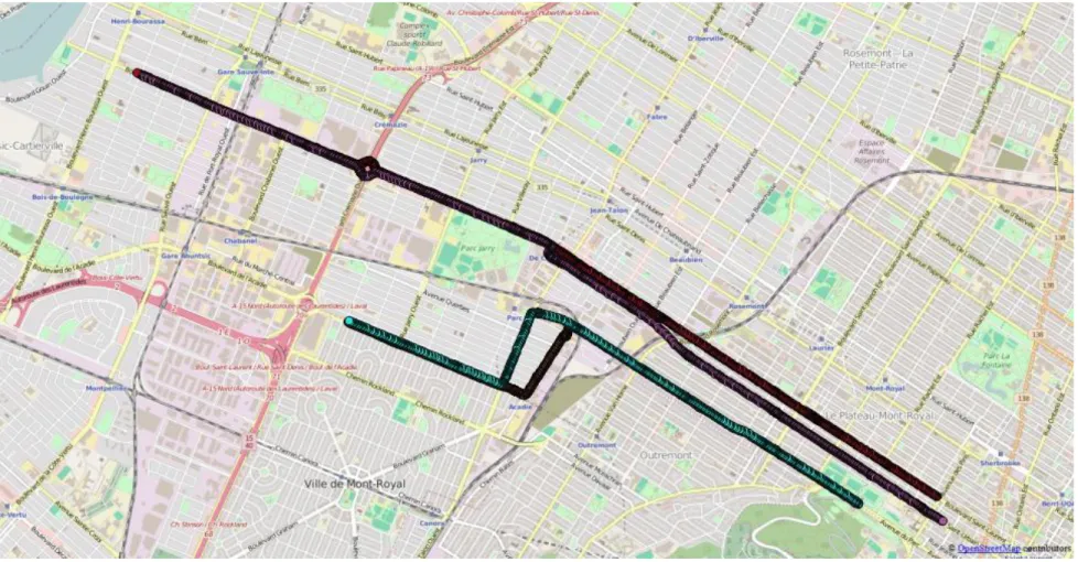
4 intersections . . . 31 Figure 3.11 Related matrices for the simple network presented in Figre 3.10 . . . 32 Figure 4.1 Case study area . . . 36 Figure 4.2 Chosen routes as the east access to Montréal downtown considering the
blockage by Mont Royal hill . . . 37 Figure 4.3 Defining the availability of recorded trajectories in the chosen routes
using QGIS . . . 40 Figure 4.4 Summary of data availability on base of start time of recording
trajec-tories on different months and days in Acadie-Parc NB direction . . . 41 Figure 4.5 Summary of data availability on base of start time of recording
Figure 4.6 Summary of data availability on base of start time of recording
trajec-tories on different months and days in St. Laurent NB direction . . . 43
Figure 4.7 Summary of data availability on base of start time of recording trajec-tories on different months and days in St. Urbain SB direction . . . . 44
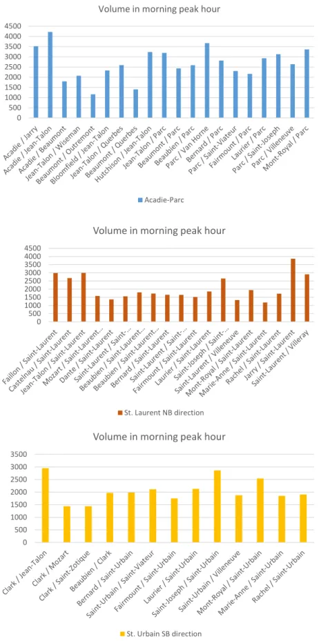
Figure 4.8 Traffic volume at each intersection in morning rush hour . . . 46
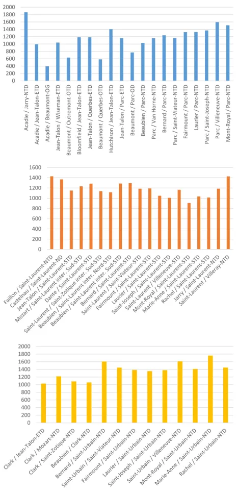
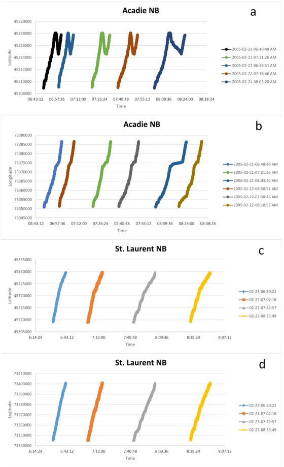
Figure 4.9 Main turn and its volume at each intersection in morning rush hour . 47 Figure 4.10 Available GPS recorded trajectories during morning peak hour (07 :30 A.M. to 08 :30 A.M.) . . . 53
Figure 4.11 Various patterns of the routes as it is clear from latitude (a and c) and longitude (b and d) of GPS traces . . . 54
Figure 4.12 Modeled network using SUMO (Output by SUMO GUI) . . . 56
Figure 5.1 Distribution of calculated probability of each available state . . . 60
Figure 5.2 The most probable state at each time . . . 61
Figure 5.3 Predicted speed in link P45 . . . 63
Figure 5.4 Predicted density in link P45. . . 63
Figure 6.1 The most probable state at each time using 50 % of available streaming data . . . 66
Figure 6.2 The most probable state at each time using 75 % of available streaming data . . . 67
Figure 7.1 Comparing the results of the proposed method by real speeds reported by GPS traces for links P45, P47, and P49 . . . 70
Figure 7.2 Comparing the results of the proposed method by real speeds reported by GPS traces for links P51, P53, and P55 . . . 71
Figure 7.3 Comparing the results of the proposed method by real speeds reported by GPS traces for links P57, P59, and P61 . . . 72
Figure D.1 Description of possible directions in counting traffic volumes at each intersection . . . 89
Figure E.1 Average experienced speed within morning rush hour on 2005-02-23 . 90 Figure F.1 Average experienced speed in different time spans of the days . . . 91
Figure F.2 Average experienced total travel time in different time spans of the days 92 Figure H.1 Node numbers and the related intersections . . . 94
Figure H.2 Link numbers and the related intersections in Acadie-Parc route . . . 95
Figure H.3 Link numbers and the related intersections in St. Laurent - St. Urbain route . . . 96
Figure J.1 Latitude and longitude of the links in the study area defined for using in validation of the results of the proposed method . . . 105
LIST OF SYMBOLS AND ABBREVIATIONS
GPS Global Positioning System
ITS Intelligent Transportation System
SM Social Media
FC Floating Car
SP Smart Phone
SC Smart Card
AVI Automatic Vehicle Identification
AVL Automatic Vehicle Location
PF Particle Filtering
LN-CTM Link Node Cell Transmission Model
PHD Probability Hypothesis Density
LWR Lighthill, Whitham, and Richards
NN Neural Network
CTM Cell Transmission Model
CA Cellular Automata
GHR Gazis-Herman-Rothery
AP Action Point
SA Simulated Annealing
TT Travel Time
State Traffic conditions in an urban road network
Status Speed value for each probe vehicle defines its status between two possible statuses
MPS Most Probable State
SUMO Simulation of Urban MObility
FFS Free Flow Speed
NB North Bond
SB South Bond
QGIS Quantum GIS
GUI Graphical User Interface
TS Time-Step
t Time index
j Probe vehicle index
aj(t) Acceleration of car j at time t
vj(t) Speed of car j at time t
T Reaction time of a driver
∆v(t − T ) Relative speed between jth car and the (j − 1)th
car located in front
∆x(t − T ) Space between jth car and the (j − 1)th
car located in front
c, f , k Model parameters in GHR model
α1, α2, α3, and α4 Model parameters in safe distance model β1, β2, β3 , β4, and β5 Model parameters in linear (Helly) model dj(t) Desired following distance for car j at time t
w Width of a car
Θ Visual angle of leader car from point of view of follower driver
A Current event in general Bayesian equation
B Experienced event in general Bayesian equation
i Link index
I Total number of links
Si
t State of link i at time t
vit Speed of link i at time t
dit Density of link i at time t
qti Flow of link i at time t
St Prior state of an urban road network at time t from
simulation b
St State of an urban road network at time t from
measurements
N Number of possible sets of TT in the urban road network
b
vjit Reported speed of probe vehicle j located in link i at time t (St1, ..., Stn, ..., StN) N possible states of traffic conditions at time t
(SP1, ..., SPn, ..., SPN) N states probabilities for N possible states of traffic
conditions
P Mt Probability of measurements at time t
(CMt1, ..., CMtn, ..., CMtN) N conditional models for N possible states of traffic
conditions at time t
(BPt1, ..., BPtn, ..., BPtN) N Bayesian probabilities at time t for N possible states of
traffic conditions
decreases to zero in link i
t0ji Time of entering probe vehicle j into link i
qx Rate of change of flow with respect to space
dt Rate of change of density with respect to time
∆t The reference period before time t for defining the probability of measurements
σvˆi
t−∆T ,t Standard deviation of measured speed between t − ∆T and
t for link i µˆvi
t−∆T ,t Average of measured speed between t − ∆T and t for link i
t? Dissipation time of the queue located ahead of the probe
vehicle
XDi The coordinate of the intersection located downstream of
the link i
L The effective average length of vehicle
Sr The uniform service rate of intersection
∆tr Remaining time of red time of the signal located at down
stream after the time that the probe vehicle starts reporting its speed as zero
tG The time that the first next green time changes to red QU i The volume of arrived vehicles after the probe vehicle
from upstream of the link i
λ Density mean of link i between tji0 and t
LIST OF APPENDICES
APPENDIX A - Detail of link characteristics in the chosen arterials
(source : Jandik (2015)) . . . 82 APPENDIX B - Structure of file of recorded GPS traces . . . 86 APPENDIX C - Detail of start time of recording trajectories in the chosen arterials . 87 APPENDIX D - Counted traffic data at intersections from 2003 dataset of traffic survey 89 APPENDIX E - Analysis of average speed (source : Jandik (2015)) . . . 90 APPENDIX F - Analysis of speed and travel time distribution within three time spans
of day . . . 91 APPENDIX G - Turning probabilities defined in order to create input files required to
simulate traffic conditions . . . 93 APPENDIX H - Introducing characteristics of the nodes and the links used in
simula-ting states by SUMO . . . 94 APPENDIX I - The codes used in running SUMO to define the probe vehicles and
travel times of the links . . . 97 APPENDIX J - Latitude and longitude of the links . . . 105 APPENDIX K - Implemented formulas using Excel for calculations . . . 106
CHAPTER 1 INTRODUCTION
With the increase in car ownership rate in megacities, people have increased their car us-age for daily activities. As a result, megacities experience high levels of traffic congestion, on a daily basis. Governments cannot build new infrastructure to cover the increasing de-mand. Therefore, new methods have emerged to deal with the imbalance in the supply and demand. Finding new policies and solutions is a high priority for decision makers and re-searchers. Various policies have been proposed to decrease the congestion on urban roads. For example, investing strategically in public transit, optimizing road network performance, eliminating bottlenecks, adding and optimizing new roadway capacity, and road pricing have been recommended (Staley, 2012). Also, real time management and route guidance have been considered as a suitable solution to increase network capacity. However, in order to assess the sustainability of these policies, a precise understanding is required about the spatio-temporal dynamics of traffic conditions on the urban road network.
It is required to know, what are the basic traffic indicators such as speed, flow, and density, in quasi-realtime on link-by-link basis of the road network. Furthermore, it is possible to perform short-term forecasting of the state of the system based on these statistics. Finally, it would enable us to pre-emptively apply various strategies to optimize the flow and maximize the throughout of the network.
Accessing the information produced by new sources, commonly known as Big Data, enables us to understand various phenomena in transportation and traffic engineering. Especially, it helps us for short-term vehicular flow modelling. Using streaming data obtained from the user-centric sources will help us improve the understanding of recently-experienced events in urban road networks. Thus, we can draw a more realistic picture of the short-term traffic conditions by developing new prediction methods. The streaming nature of the data provided by this new source alongside with traditional data that need noticeable finance and effort, can be exploited for better short-term predictions.
In order to make traditional models of demand and activity behaviour, the required data is collected using a small subset of the whole population for a short duration of time every 5 to 10 years. Nowadays, new technologies like GPS, sensors, smart phones, and social media platforms provide us with the opportunity to increase the volume of collected data to develop more accurate transportation models (Vij and Shankari, 2015). Predicting traffic conditions is one of the fundamental parts in Intelligent Transportation System (ITS) (Li et al., 2015). Using more data enables us to develop better models to predict future conditions of the road network more precisely.
Existing traffic simulations are calibrated once using traditional datasets that are predomi-nantly cross-sectional in nature and collected once every couple of years. In these simulations there is no feedback from the recently experienced states of traffic conditions in the network and they are only recalibrated whenever the new cross-sectional dataset is available. These simulations are used to predict the future of the urban network without considering the short-term important feedbacks from local spatial and temporal variations. Therefore, there is a need to consider and apply these feedbacks and update our simulations based on the new information about the short-term state of the urban network. Using recently avail-able streaming data from various sources such as smart phones, traffic cameras and social networks, we can simulate short-term traffic conditions with feedback to incorporate recent conditions.
Streaming data/longitudinal data sources provide us with the ability to develop new meth-ods of predicting traffic conditions. Streaming data are the most recently addressed sources of data that can be used to improve our knowledge of traffic conditions. Moreover, their real-time features give us the opportunity to manage and control traffic in order to increase the performance of transportation systems (Shi and Abdel-Aty, 2015). Streaming data can be collected using network based or user-centric techniques (Danalet et al., 2014). Stream-ing data collected by user-centric techniques can provide individual level patterns of traffic behaviour.
More formally, Social Media (SM), Floating Car (FC), Smart Phone (SP) and Smart Card (SC) are categorized in the set of user-generated data sources. Mining, managing and analyz-ing this type of data, in order to understand the complexity and dynamics of trip patterns, is a noticeable job considering the amount, richness, and dynamism. Therefore, we need to create new advanced methods to analyze these data; develop individual-level models; and simulate individual transportation and activity patterns (Gkiotsalitis and Stathopoulos, 2015). User-centric data generated by the users of the urban road network, enable us to access the required information that we need to define the spatio-temporal fluctuations of traffic indi-cators at link level. We can define different possible states of traffic conditions in an urban network. By accessing to real-time data about traffic indicators in part of urban road net-work, we can define which possible state of traffic conditions in whole of urban road network is more probable, regarding available streaming data received form user-centric sources. In this research, we concentrate on using the Bayesian approach to define the most probable state of an urban network using streaming data provided by user-centric sources as well as the simulation of traffic dynamics. We define the prior model using a traffic microsimulator to create possible states of traffic conditions in the urban road network. Also, we calcu-late the probabilities of measurements using user-centric data available as streaming data
and measure a conditional model for each possible state of urban traffic conditions at each time-step, using the output of the traffic microsimulator and streaming data. The proposed methodology enables us to predict link-by-link traffic conditions at a given time, based on available streaming data.
This research has two main cores: a traffic microsimulator that can generate the traffic con-ditions in possible states of the urban road network and a proposed Bayesian approach that enables us to decide about the most probable state at each time-step. Therefore, in the fol-lowing chapter on the review literature we focus on these two main topics to elaborate which traffic modelling frameworks and prediction methods have been used and what are our best options in these two main cores of this study.
The rest of this thesis is organized as following: First, we will present a literature review to describe how various approaches have been used for short-term traffic predictions. Next, our methodology development is presented that explains how the proposed Bayesian approach is used to define the most probable state of the urban road network. A case study of Montréal will be explained and after reviewing and analyzing the available data, some discussion about the results of this study and the sensitivity of the analysis will be presented. The validity of the results of the proposed method will be tested and finally, conclusions and future research directions are presented.
CHAPTER 2 LITERATURE REVIEW
This chapter has been divided into two main sections so as to cover the existing literature dedicated to predicting traffic flow conditions in short-term and different modelling frame-works. The first section presents the methods of short-term prediction of traffic flow. Deciding about the best underlying modelling framework is an important task. Hence, the second sec-tion describes advantages and disadvantages of the different traffic modelling frameworks that work at various levels of spatio-temporal aggregation and employ different assumptions in modelling.
2.1 Short-term prediction of traffic flow
Level of complexity of models, spatio-temporal coverage of available data, characteristics of data used for calibration and validation, existence of non-linearity relationship between indicators, and temporal variations in observations for an indicator in an urban road network are some examples of the factors that affect the reliability of traffic condition predictions (Canaud et al., 2013). Consequently, developing new methodologies for overcoming these issues is essential.
Existing studies use different sources of data from various detection technologies. In next part, we present a brief review of available detection technologies. Afterwards, we focus on different method of short-term prediction of traffic flow in existing literature.
2.1.1 Detection technologies
For monitoring urban traffic, in order to understand its macroscopic characteristics such as link level travel time, speed, and flow (Nantes et al., 2013) and to answer the numerous needs of the urban community, traffic information systems play a specific and paramount role (Herring, 2010). Recently, there is a growing endeavor in estimating and forecasting ar-terial network traffic conditions, by using probe data (Hofleitner et al., 2012). Short-term traffic management and control can greatly benefit by predicting traffic flow indicators such as travel time, speed, and volume.
In order to predict traffic conditions, we need detection/tracking technology to measure traf-fic indicators in urban road network. There are three types of technologies: in-roadway and over-roadway detectors and off-roadway technologies (Shi and Abdel-Aty, 2015). Loop de-tectors are examples of in-roadway dede-tectors. Installing and repairing these types of sensors
can disturb traffic. In specific situations, they have noticeable failure rates; for instance, in unsuitable weather and road surface conditions. Located over the roadway or alongside and placed at some distance from the nearest traffic lane, the over-roadway sensors have evolved from video image processing to more up-to-date microwave radar sensors. Their most im-portant advantage is minimizing traffic disruptions for installation and maintenance. Probe vehicle is an example of the off-roadway technologies that need in-vehicle devices in addi-tion to fixed infrastructures compared to in - and over - roadway technologies. GPS, cellular phones, Bluetooth, Ground-Based Radio Navigation, Automatic Vehicle Identification (AVI) and Automatic Vehicle Location (AVL) are some examples of this type of detection techno-logies.
In - and over - roadway technologies have the ability of traffic counting, but speed measu-rement by these two types of technologies is less accurate than probe vehicle as an example of off-roadway technologies (Martin et al., 2003). While all vehicles do not have in-vehicle devices, access to complete and accurate information about some traffic indicators is not possible using off-roadway technologies (Shi and Abdel-Aty, 2015).
Various existing studies have used different sources of data and have employed different ap-proaches for predicting traffic conditions using available data. In next part, we concentrate on existing methods of short-term prediction of traffic conditions.
2.1.2 Short-term traffic prediction methods
Park and Lee (2004) created travel time models on arterial roads using loop detectors in the network and a dedicated probe vehicle with installed communication devices. They im-plemented neural networks to calibrate the model and validated their model under limited conditions. Coifman (2002) developed a method using data from a loop detector installed at a single point of a freeway to define link travel time. The proposed method is not able to consider the effect of a delay or a queue resulted by an incident. Coifman and Krishnamur-thy (2007) developed a method for detecting congestion in a link located between two loop detectors installed in a freeway by reidentificating long vehicles. In arterials, access to land use is not limited as freeways. Therefore, reidentification of some vehicles that exit arterials between two consecutive loop detectors is not possible between all loop detectors at the end of links. Hence, it can be concluded that their proposed method is not usable for arterials. Jenelius and Koutsopoulos (2013) used GPS traces to develop an arterial road travel time model in Stockholm. They implemented a maximum likelihood based approach for correlating link characteristics, mean link conditions, and weather conditions to the link speed. Their statistical approach is noticeable that considers the effects of mentioned conditions. But the approach is not able to consider the effects of the traffic conditions from the surrounding
network that is possible by implementing a traffic simulation. In their statistical approach, travel time between two points was considered as a combination of stochastic links’ travel times and deterministic intersections’ delays. Their assumption about delay at intersection cannot reflect what happens in reality.
Pascale et al. (2013) estimated link densities in highway using noisy and sparse measure-ments of density collected from road-embedded sensors, by proposing recursive Bayesian approach combined by a particle filtering (PF) approach (a sampling method). In traffic simulation, they used a stochastic form of Link Node Cell Transmission Model (LN-CTM). They implemented numerical tests and concluded that even in situations of very sparse sen-sor deployment, estimating the traffic conditions is possible using mathematical methods. They modeled traffic conditions at a macroscopic level that does not enable their proposed approach for using individual level data.
Canaud et al. (2013) created a new tool for estimating vehicular density on urban roads. They proposed the use of Probability Hypothesis Density (PHD) for solving the state esti-mation problem. By evaluating their PHD filter against particle filter (PF), they concluded that the PHD filter can be considered as a suitable alternative. The proposed method is not appropriate for developing an approach to use real-time traffic data for defining the short-term state of urban road. The approach is suitable for studying a specific link and cannot enable us to define traffic indicators in the whole urban road network when we have access to measurements in only a part of network.
Herring (2010) proposed a hybrid approach by implementing a general system architecture to analyze traffic data and disseminate accurate, timely traffic information through the Inter-net. This approach leveraged the advances in the fields of machine learning and traffic theory (using hydrodynamic theory) to estimate arterial traffic conditions. Two different approaches using historical data in modelling traffic conditions applied: Regression and Bayesian. The second approach has been introduced as the better one based on the results of this study. It is noticeable that learning from historical data when there is considerable changes in traffic volumes cannot be accurate. Also, there is a need to combine the Bayesian approach with traffic simulation for achieving more trustworthy results that has not been applied to this study.
Hofleitner et al. (2012) used a dynamic Bayesian network. They used sparsely observed probe vehicles, and proposed a probabilistic modelling framework for approximately defining and forecasting travel time distributions on urban roads. Their method represented the spatio-temporal dependency on the network by considering traffic state as hidden, which is affected by travel time observations. It provided a flexible framework to learn traffic dynamics from historical data and to perform real-time estimations with streaming data. While in the
Baye-sian updating method the prediction at each time step is updated based on available data, the proposed method in this study considered the dynamism that affects the current traffic state. The sampling rate of probe vehicles in their study did not provided detailed informa-tion about the locainforma-tion where vehicles encountered delay. Compared to the baseline approach, their method provided 35 % increase in estimation accuracy. This approach in short-term modelling traffic conditions is notable as it only considers experienced traffic conditions re-ported by GPS traces. But this approach is not able to provide predictions about the part of the network that is not covered by probe vehicles at all.
Nantes et al. (2013) captured the spatio-temporal relationship between volume and travel time. They proposed an approach based on a simple Bayesian network for analyzing and pre-dicting the complex dynamics of flow or volume that was based on travel time observations from Bluetooth sensors. Their proposed Bayesian approach was simple as it considered the current state dependent only on the previous state and the travel time indicator dependent only on current state (first-order transition model). They considered distribution of obser-vations by sensors Gaussian. The complex dynamics of arterial volume and travel time was estimated and predicted effectively by their proposed Bayesian network. They estimated the joint distributions, over sequences of volume values. Their proposed method focuses on the streaming data in part of the urban road network. The method is not able to produce results about part of the network that has not been covered by the sensors.
Polson and Sokolov (2014) developed a PF and learning method to estimate current traffic conditions (density) and key parameters of Lighthill, Williams, Richards (LWR) model. They proposed an algorithm that could improve on existing methods by permitting real-time up-dating of the posterior distribution of the critical density and capacity parameters through on-line learning. Even at shock waves, their PF algorithm was able to estimate uncertainty of the traffic state by considering mixture distribution. Moreover, by using the Bayesian pa-rameter learning and estimation, improving the estimation bias was possible. By fixing the parameters it led to mis-estimation. If the relationship between flow and density changes over time or there is a queue or bypassing traffic, the proposed method is not realistic even in highways.
Staňková and De Schutter (2010) proposed a PF method for predicting/estimating traffic density using Daganzo’s cell transmission model, based on jump Markov linear system (a nonlinear switching Markov system of multiple linear models). They used importance sam-pling in their PF method to select samples with higher normalized importance weights, the ratio of a sample probability over the probability of an arbitrary proposal distribution. They concentrated on the performance of their method and the system properties by comparing its result with the output of microsimulation by Aimsun 6. Although, they assumed that
conges-tion happens in one segment only, the extension of their approach to the model that contains all possible congestion modes was straightforward. They mentioned that more research is needed to apply the proposed method to the more general problems respecting performance in time, variance, etc.
Chen and Rakha (2014) used a new PF approach to define travel time in highway by applying real-time and historical data. They used a different sampling strategy to filter out invalid or low wighted particles and replace them with historical data that had the same data sequence in real-time measurements.
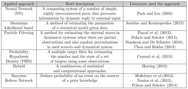
Modelling urban road traffic using traditional methods of data collection has some disad-vantages. To overcome these disadvantages, there are various approaches already proposed, which can be categorized into Statistical approach to Neural Network, Bayesian approach and so on. A summary of these methods is presented in Table 2.1.
Vlahogianni et al. (2014) reviewed the literature related to short-term forecasting methods.
Table 2.1 Applied approaches in short-term prediction of traffic flow
Applied approach Brief description Literature used the approach Neural Network A computing system of a number of simple,
(NN) highly interconnected parts that processes Park and Lee (2004) information by dynamic reply to external input
Maximum A method of estimating the parameters Jenelius and Koutsopoulos (2013) Likelihood based of a statistical model given data
Particle Filtering A method for estimating the internal states in Pascal et al. (2013), dynamical systems when there are partial Polson and Sokolov (2014), observations and also random perturbations Stankova and De Schutter (2010),
in used sensors and dynamical system Chen and Rakha (2014) Probability A multiple target filter for estimating
Hypothesis the number and the state of a set Canaud et al. (2013) Density (PHD) of targets using some observations
Hybrid A combination of statistical Herring (2010) and computational approaches
Bayesian Defines probability of an event on the context Hofleitner et al.(2012), Believe Network of a prior knowledge Nantes et al. (2013),
Polson and Sokolov (2014) They mentioned 10 important challenges related to this topic. These challenges are related to integration of predicting models; the problem of forecasting traffic and variable choice; data issues and the impact of new technologies on available datasets; developing novel prediction algorithms; and the effect of artificial intelligence model on integrating models into prediction schemes.
Reviewing existing literature, summarized in Table 2.1, it can be concluded that the dynamic prediction of link by link traffic conditions in whole of a complete network using streaming data and Bayesian approach is not possible by the proposed methods of existing literature.
Although, there are some Bayesian approaches have only been used at corridor or neighbo-rhood level, the proposed methods are not able to predict traffic conditions in whole of a network when we have access to streaming data in a part of network. The Bayesian approach in most of the reviewed existing literature has been used to explore historical and real-time data for estimating traffic state in a part of the urban road network. While combination of a simulation based on traditional data and a Bayesian approach that uses streaming data available in a part of network and the simulation outputs has not been applied in the related literature to predict traffic conditions in the whole network. We need to do this combina-tion to increase the ability of the new proposed approach of this study in traffic condicombina-tions prediction when we have no information in a part of the network regarding the randomness in space and time of streaming data. Therefore, we aim to study the problem and we will explain our rational for the selected method. In the following part, we focus on reviewing the literature in order to choose a suitable traffic flow modelling framework.
2.2 Traffic modelling frameworks
We need to model traffic conditions in an urban network; therefore, a review of existing traffic modelling framework is presented here.
2.2.1 Cell transmission model (CTM)
In this framework, the network is divided into cells based on the differences in link properties and connections to other links (Alecsandru, 2006). The occupancy of each cell at each time-step is defined based on its occupancy, inflow at the last time-time-step, and the outflow from the connected downstream links at the current time-step. This approach is reasonably suited and appropriate for planning analysis problems and its macroscopic nature makes it more efficient from a computational point of view. It also requires minimal effort for calibration since it has comparably less parameters. CTM makes traffic flow modelling more realistic1 in
various implementations containing both static and dynamic traffic assignment procedures. This method is suitable for some specific applications, for instance, it is suitable for analysis of disaster evacuation solutions at the planning level. In CTM, the network is divided into cells resulting in possible geometric limitations (Alecsandru, 2006). If the network is divided into many small cells, we need additional memory. Therefore, CTM is not suitable for modelling large-scale urban network. We want to model different facility types. For instance, when we have freeways and intersections on city streets, modelling of large-scale networks will be 1. Because the way it defines the state of each cell at each time-step is more compatible with what happens in reality.
computationally inefficient.
2.2.2 Cellular automata (CA)
It is used in traffic flow microsimulation to model the behaviour of cars traveling on a road network. The basic idea is to discretize space in cells of equal size, each of which can be occupied by at most one vehicle. Cars drive through these cells by choosing their speed according to the space available in front of them. The advantage of cellular automata (CA) is that link capacities are generated from the properties of the links and drivers’ behaviour. The major drawback of this method is its computational cost as every agent is simulated in every time step, which is usually a second (Maerivoet and De Moor, 2005). Ignoring the computational cost, developing a model by CA can be useful for modelling special links and is not suitable for modelling a whole network.
2.2.3 Queue-based simulations
In this method, the intersections would be modeled alone where (Charypar et al., 2007): 1. Links are modeled as they "process" cars moving through the network.
2. A queue stores cars coming from each link together with their respective entry times. 3. Each link’s capacity and space available for cars are parameters of the model.
4. The related links cooperate in each time-step by considering different link constraints such as capacity, free speed, travel time, intersection precedence and space available at the next link, in order to define the next position of cars in the network.
Queue-based models are faster than CA mainly because the number of simulated units is smaller (links vs. cars). A special form of queuing simulation (event-based) is based on the occurrence of events (Charypar et al., 2007). There is no fixed time-step and the cars are only processed when an associated event (e.g. arrival, departure, etc.) occurs. Entering or leaving a link is also considered an event. It means that event processing rate is related to the flow in all time-steps.
2.2.4 Car-following models
This type of models describe the behaviour of drivers in an urban network (Brackstone and McDonald, 1999). They assume that the behaviour of each car is a function of the proceeding car. To model the reaction of driver to the followed car, there are various types of models that can be classified as car-following models. Gazis-Herman-Rothery (GHR) model (Gazis et al.,
1961), safety distance or collision avoidance models (Kometani and Sasaki, 1959), and Linear (Helly) models (Helly, 1959) are classified in this category. Also, there are other approaches in this category, the most important types of which are Psychophysical or Action Point (AP) models (Michaels, 1963) and Fuzzy logic-based models (Kikuchi and Chakroborty, 1992).
GHR model
In the GHR model, acceleration of car j at time t, aj(t), is defined by (Brackstone and
McDonald, 1999):
aj(t) = c(vj(t))f
∆v(t − T )
(∆x(t − T ))k (2.1)
Where vj(t) is the speed of car j at time t, ∆v(t−T ) and ∆x(t−T ) are the relative speed and
the space between jthcar and the (j − 1)th car located in front, T is reaction time of a driver, and c, f , and k are the model parameters. This type of car-following models introduced by Chandler et al. (1958), has been adopted and improved by Herman et al. (1959), Gazis et al. (1961) and others.
Safe distance model
In safe distance models, the safe following distance, ∆x(t − T ), is defined by (Brackstone and McDonald, 1999):
∆x(t − T ) = α1.(vj−1(t − T ))2+ α2.(vj(t))2+ α3.vj(t) + α4 (2.2)
Where α1, α2, α3, and α4 are the model parameters.
This set of car-following models were introduced by Kometani and Sasaki (1959) and impro-ved by Gipps (1981). They were used in some simulating models, for instance, in INTRAS and CARSIM in the USA (Benekohal and Treiterer, 1988).
Linear (Helly) model
In Linear (Helly) model, aj(t) is defined by (Brackstone and McDonald, 1999):
aj(t) = β1.∆v(t − T ) + β2.(∆x(t − T ) − dj(t)) (2.3) dj(t) = β3 + β4.vj(t − T ) + β5.aj(t − T ) (2.4)
Where dj(t) is desired following distance for car j at time t and β1, β2, β3, β4, and β5 are
the car by considering the reaction time of the driver. This model proposed by Helly (1959), then calibrated by Hanken and Rockwell (1967) and others. Also, in the mid nineties, a combination of the linear model and GHR model proposed by Xing (1995).
Action Point (AP) model
In AP model that was proposed by Michaels (1963), a driver in approaching a vehicle considers its visible dimension by realizing the relative speed that affects the visual angle of the vehicle (Brackstone and McDonald, 1999). Figure 2.1 shows how the visual angle and its changes over time can be defined using next equations:
Θ = 2 arctan( w 2∆x) (2.5) dΘ dt = − w∆v (∆x)2 (2.6)
There is a threshold for (∆x)∆v2 in the literature (Brackstone and McDonald, 1999). By
excee-ding this threshold, the driver decelerates and adjusts its speed. Also, the other threshold for adjusting minimum space between two consecutive vehicles is considered. Although, it seems that this model simulates drivers’ behaviour correctly and is able to explain what happens in reality, proving or disproving its validity is difficult and calibrating its individual elements and the thresholds has been rarely successful.
Follower Vehicle Leader Vehicle Δx Ɵ
Figure 2.1 Visual angle and the related factors
Fuzzy logic-based model
Fuzzy logic-based models consider some logics in describing the driver behaviour (Brackstone and McDonald, 1999). For example, the term "too close" or "not close" can be defined and quantified. If the time space between two vehicle is less than 0.5 s, the separation is "too close" and its membership number is 1 and if it is more than 2 s, the separation is "not close" and its membership number is 0. Using Fuzzy output set we can define the pattern of driver behaviour by applying the mentioned sets by logical operators. This approach used to ”fuzzify” the GHR model (Kikuchi and Chakroborty, 1992), and also the other models.
2.2.5 Comparison between traffic modelling frameworks
In this section, we compare the four frameworks in traffic modelling (CTM, CA, Queue-based, and Car-following) to find the most appropriate simulator to supply its outputs parallel to streaming data, that is at individual level, and feed them to the Bayesian approach that was chosen as the suitable approach in section 2.1.2 for this study.
Hofleitner et al. (2012) used CTM for developing a Bayesian model using streaming data in arterial travel time estimation. Also, Alecsandru (2006) tried to consider the effect of random driving behaviour at macro level and developed a CTM based approach to apply this behaviour. The following results can be mentioned from his study:
1. It is assumed that the randomness of the aggregate behaviour at a macroscopic level is the result of random behaviour of individual drivers. Therefore, random variation in the observed short-term capacity is the result of the randomness in minimum headway; and the random variation in local jam densities is the result of randomness in minimum space headway.
2. In CTM, by the modified flow advancing equation, the effect of randomness can be applied to the free flow speed, flow capacity, space capacity, and the speed of the backward moving wave.
3. Results of the case study by constant and dynamically varying wave speed show that there are some fluctuations in cell occupancies over time. However, in both cases the total travel time was approximately the same.
Stochastic CTM model has been developed using the Bayesian approach to estimate travel time and density in a network. But considering that we need to produce the outputs from the target traffic modelling framework at a microscopic level, using CTM and the stochastic form developed by Alecsandru (2006) is not a suitable choice for a traffic modelling framework. Cellular automata (CA) considers the behaviour of drivers stochastically. The system that generates this stochasticity has not been developed enough. For instance, it contains some rules for increasing the speed of a vehicle and braking to avoid collisions. The stochasticity in the system, for example in braking events, is defined by a random number drawn from a uniform distribution that is compared with a stochastic noise parameter (called the "slow down probability") that defines the probability of decreasing vehicle speed. Therefore, from the behavioural point of view, CA modelling framework is not able to consider the probabi-listic nature of driver behaviour accurately (Maerivoet and De Moor, 2005).
To apply this modelling framework, we need considerable computational time for simulation. Also, we mentioned that it is suitable for simulating parts of a network and special links. It is not computationally suitable for the entire target network. Therefore, using this framework
is not recommended for generating the output we need to use with available streaming data. Queue-based modelling framework focuses on simulating events at intersections. Although, this approach gives us outputs at each car level, it can only model the intersections. There-fore, we cannot use it to feed its outputs with available streaming data that are at microscopic level.
Car-following models enable us to consider different patterns of drivers’ behaviour in order Table 2.2 Summary of comparison between four traffic modelling frameworks
Framework Simulation Stochasticity Computational Output level limitation compatibility CTM Dividing a Is possible Is not suitable Cannot generate at
link into cells in large scale microscopic level CA A cell for Is not realistic Suitable for At microscopic level
one vehicle part of network
Queue-based Vehicle at Is possible Suitable for At microscopic intersection large scale level Car-following Vehicle Is possible Suitable for At microscopic
in link large scale level
to increase the realism of a chosen model by applying motivational and attitudinal factors. This approach is confirmed by available evidence and it is more realistic framework in mo-delling traffic conditions due to these various patterns. But it can be noted that relating the mentioned features to observed dynamic behaviour has been rarely addressed in the existing literature (Brackstone and McDonald, 1999). Efforts have been made to develop these types of models. However, it can be concluded that car-following models can better capture the microscopic behaviour in links regarding available streaming data. The summary of these comparisons is presented in Table 2.2.
We propose using car-following modelling framework that is able to provide outputs at a microscopic level as the prior distribution in the Bayesian framework. It does not have the limitations of CTM and CA in computing ; and can consider stochasticity in modelling traffic conditions.
Therefore, applying microscopic car-following modelling framework can provide better results by considering individual behaviour and its effects on link parameters. We need to know what happens at low level in the network in order to consider the effects of streaming data that are at microscopic level on developing more realistic understanding about the urban road network.
2.3 Contribution of this study
It has been demonstrated that traffic conditions in urban network cannot be predicted with naive and deterministic models. For instance, patterns of traffic conditions differ for a given link in the same duration of time for two different working days of a week. Also, the patterns change from a working day of a month to an other month for the same season. These fluctua-tions cannot be simulated by a deterministic model. In the age of streaming and longitudinal data, the stochastic nature of traffic conditions needs to be captured by new models. Exis-ting models simulate traffic conditions in urban networks using traditional data and their outputs for a network are fixed sets of link properties. The fluctuations in the patterns of traffic conditions dictates considerable uncertainty for using the outputs of a simulation as the urban network state.
Using the user-centric streaming data, we can create a more realistic image of network state in short-term. We can update the existing model that has been developed using traditional data by implementing a feedback from these new sources of non-traditional data. Therefore, the updated prediction of urban network state leads us to recommend a more realistic state. Figure 2.2 shows the contribution of this thesis. Based on Figure 2.2, we try to prove the ability of the proposed methodology for achieving more realistic understanding of traffic conditions in an urban network by fusing the outputs of simulation of various possible states of traffic conditions and streaming data using the Bayesian framework.
We can define link-by-link parameters of the urban road network stochastically. Moreover, the proposed method enables us to assess long term policies. Although, the output of this study is not an operational tool, it can provide us with the opportunity to think about developing one that would help us control and manage congestion in urban road networks dynamically and help users in optimizing their route choice decisions. The main output of this study as a prototype tool, proves us the capability of the proposed method for traffic conditions prediction by using streaming data parallel to the traffic simulation that is based on traditional data.
We propose a Bayesian approach to use the simulation outputs of various possible urban network states and available streaming data for defining the most probable state of the ur-ban network. The next chapter mainly consist of: (1) Streaming data and improvement in traffic prediction methods; (2) Bayesian updating approach; (3) Structure of traffic model using car-following framework.
In the proposed Bayesian approach, the related probabilities of prior simulations and the probabilities of available measurements, streaming data, are defined. Also, the conditional models using the simulation outputs of various possible states and streaming data are
mea-THE MOST PROBABLE STATE
Available streaming data Probable microsimulated urban road network states
FUSING
STREAMING DATA
&
TRAFFIC MICROSIMULATION
USING
BAYESIAN APPROACH
Figure 2.2 Statement of contribution
sured. Finally, using the proposed methodology we can define the probability of each possible state and predict the most probable urban network state at each time-step.
CHAPTER 3 METHODOLOGY
3.1 General framework
Implementing different strategies to manage congestion on urban networks, improving their states, and maximizing their capacities are possible by understanding traffic conditions and short-term forecasting in each link (Farooq, 2013). Figure 3.1 shows the procedure used in a conventional network modelling framework that only uses traditional data. A traffic model is calibrated and validated only once using traditional data and it is implemented for short-term prediction. We know that there are different patterns of traffic behaviour at the same time during different weekdays or different months of a season. Figure 3.2 shows the improved procedure with feedback by implementing recent events in the network that we try to cover it as much as possible on the frame of this thesis. Conventional method of traffic prediction (Figure 3.1) cannot consider the effects of these differences. By implementing streaming data available from sensors (Figure 3.2), we can consider the effect of the mentioned differences on traffic conditions in traffic conditions prediction methods that we propose by using a Baye-sian approach and user-centric streaming data.
Streaming data as a non-traditional source of information provides us with the ability to
Traditional data Conventional traffic model Without considering recently experienced state Existing understanding about traffic conditions
Figure 3.1 Conventional modelling framework without considering impacts of recently expe-rienced traffic conditions, based on Furnish and Wignall (2009)
improve traffic conditions prediction methods. Probe vehicles (vehicles with any form of GPS devices) are able to generate streaming data required to use for this improvement. If there are enough probe vehicles that have in-vehicle devices, they can prepare real-time traffic information at an individual level. However, while only some vehicles have these devices,
Traditional Data Existing traffic model Likelihood Streaming Data Sensors Bayesian framework Updated traffic state
Figure 3.2 Improved network modelling framework using a Bayesian updating framework and user-centric streaming data for considering the impacts of recently experienced traffic conditions
accessing complete traffic indicators by just using this data is not very accurate. Therefore, there is a strong need to efficiently integrate and fuse streaming data with forecasting tools that use traditional data. This integration can help us to estimate the network state more precisely. It noticeably impacts the value of transportation system analysis.
There are direct and indirect benefits from using streaming data. Direct ones can be classified into congestion reduction, incident prediction, and travel time estimation. Strengthening the traffic simulation methodologies by developing, calibrating and validating new generation of models can be categorized as indirect benefits (Shi and Abdel-Aty, 2015).
Previously used tools like embedded sensors, for example loop detectors and camera tech-nology, have considerable disadvantage that were mentioned in section 2.1.1. User-centric sources of data have remarkable advantages in comparison to other sources. For instance, by accessing the streaming data produced by probe vehicles, achieving a sample of speed in the network is possible (Farooq, 2013). Therefore, in this thesis, streaming data available from probe vehicles will be used to improve the prediction of traffic conditions.
Figure 3.2 shows the proposed procedure of traffic prediction with feedback from streaming data. By using streaming data and the outputs of a traffic model, we can consider the impact of recently experienced traffic conditions in a part of network on our understanding about traffic conditions in whole of the network. A Bayesian approach is proposed to use the out-puts of a traffic simulation and streaming data. By defining likelihoods of all possible states of an urban road network we can recommend the one with a higher likelihood as the most probable state of the urban network at each time-step. The Bayesian updating approach is
explained in the next section.
3.2 Bayesian updating approach
The Bayesian framework, which was introduced by Thomas Bayes is a powerful tool for inter-preting a current event in the context of experienced events or recently available knowledge (Stone, 2013). Different studies have concluded that the Bayesian framework is suitable for effectively prediction of the complicated arterial conditions specifically the related hidden dynamism (Herring, 2010; Hofleitner et al., 2012; Nantes et al., 2013; Polson and Sokolov, 2014).
The reason that leads us to use this approach for updating our understanding about traf-fic conditions in an urban road network is its ability in relating the experienced events to current event. This approach enables us to consider posterior understandings of the network state and its probability regarding available measurements, streaming data, as the recently experienced events. By combining this approach with a traffic simulator that generates the different posterior understandings, we can predict traffic conditions of a whole network while we have no access to complete data of measurements in the network (Nantes et al., 2013). This framework generally is explained by the following equation :
P (A | B) = P (B | A).P (A)
P (B) (3.1)
Where A is the current event and B is the experienced event.
This framework can be used when there are new updates on traffic conditions. We can apply the effect of new information on updating the understanding of reality about traffic conditions as the most probable state of the urban road network.
Urban network combines two types of elements: links and intersections. In a network, at a certain time t, we are interested in determining the most probable state of the system i.e. traffic conditions in a road network link by link. The state of each link consists of three elements: flow, density, and speed. For a link i at time t, we can define the state variables as
Si
t = (vti, dit, qit). This state is the combination of three elements: vti as speed, dit as density,
and qi
t as the flow in link i at time t. The state of the network at time t can be defined as St = (St1, ..., Sti, ..., StI). We consider S and ˆS as the state of the urban network respectively
from simulation and measurement that are the combination of the states of all links.
We want to find the probability distribution P (St | Sbt) (equation 3.2). Where Sbt is the measurement received as user-centric streaming data. In this condition, applying the Bayesian
framework discussed above is possible. We can write:
P (St|Sbt) =
P (Sbt| St).P (St)
P (Sbt)
(3.2)
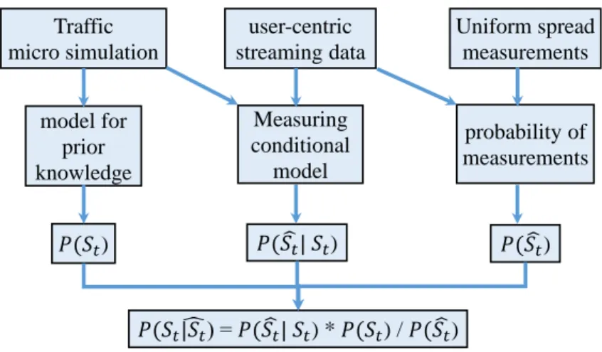
Where P (St) is the prior knowledge, P (Sbt | St) is the measurement model and P (Sbt) is the probability of measurements. This proposed approach mathematically encapsulate the pro-cesses in Figure 3.3. model for prior knowledge Traffic micro simulation 𝑃(𝑆𝑡) user-centric streaming data Measuring conditional model 𝑃( 𝑆𝑡| 𝑆𝑡) Uniform spread measurements probability of measurements 𝑃( 𝑆𝑡) 𝑃(𝑆𝑡|𝑆𝑡) = 𝑃( 𝑆𝑡| 𝑆𝑡) * 𝑃(𝑆𝑡) / 𝑃( 𝑆𝑡)
Figure 3.3 Defining the probability of a network state as prior knowledge considering available measurements using Bayesian framework
Based on Figure 3.3, we microsimulate traffic conditions in each possible state of urban network; implement user-centric streaming data; and assume uniform spread in measure-ments. This means that measurements are distributed by an equal time gap between each two consecutive measurements. This is a realistic assumption when each probe vehicle reports its features at the start and the end of a fixed time duration. Then, we define the probability of different existing traffic conditions in various possible states of urban networks; measure the conditional model; and define probability of measurements.
We follow the same basic approach developed by Danalet et al. (2014) on using Wi-Fi traces to predict pedestrians’ activities on a campus. They considered the Bayesian framework for modeling the relationship between the probability of potential activity in the context of available streaming data as measurement about pedestrian activities. They considered that normal distribution is able to describe the errors in latitude and longitude of activity location. Also, they assumed that the errors in latitude and longitude are independent. P (St) will be
computed using historical datasets that we use to create a new model as traffic microsimula-tor, while P (Sbt | St) will be computed based on the GPS traces stream giving us the sample measurements at time t and microsimulation outputs.