HAL Id: tel-02406878
https://tel.archives-ouvertes.fr/tel-02406878
Submitted on 12 Dec 2019HAL is a multi-disciplinary open access archive for the deposit and dissemination of sci-entific research documents, whether they are pub-lished or not. The documents may come from teaching and research institutions in France or abroad, or from public or private research centers.
L’archive ouverte pluridisciplinaire HAL, est destinée au dépôt et à la diffusion de documents scientifiques de niveau recherche, publiés ou non, émanant des établissements d’enseignement et de recherche français ou étrangers, des laboratoires publics ou privés.
To cite this version:
Tarun Jairaj Narwani. Dynamics of protein structures and its impact on local structural behaviors. Human health and pathology. Université Sorbonne Paris Cité, 2018. English. �NNT : 2018USPCC160�. �tel-02406878�
Thèse de doctorat
de l’Université Sorbonne Paris Cité
Préparée à l’Université Paris Diderot
Ecole doctorale [Hématologie, Oncologie et Biothérapies et ED 561]
DSIMB / INSERM UMR S_1134
Dynamics of protein structures and its
impact on local structural behaviors
Par Tarun Jairaj NARWANI
Thèse de doctorat de Biotechnologies et Biothérapies
Dirigée par Alexandre G. de Brevern
Présentée et soutenue publiquement à Paris le 27 Juin 2018
Président de jury : Rodriguez-Lima, Fernando / PR / Université Paris Diderot Rapporteurs : Callebaut, Isabelle / HDR / CNRS, Université Pierre et Marie Curie Rapporteurs : Leclerc, Fabrice / HDR / CNRS, Université Paris-Sud, Saclay Examinateurs : André, Isabelle / HDR / CNRS, INSA, Toulouse
Examinateurs : Offmann, Bernard / PR / Université de Nantes
Dynamique des structures protéiques et son impact sur les comportements
structuraux locaux
Les structures protéiques sont de nature hautement dynamique contrairement à leur représentation dans les structures cristallines. Une composante majeure de la dynamique structurelle est la flexibilité des protéines inhérentes. L'objectif principal de cette thèse est de comprendre le rôle de la dynamique inhérente dans les structures protéiques et leur propagation. La flexibilité des protéines est analysée à différents niveaux de complexité structurelle, du niveau d'organisation primaire au niveau quaternaire. Chacun des cinq premiers chapitres traite un niveau différent d'organisation structurelle locale avec le premier chapitre traitant des structures secondaires classiques tandis que le second analyse la même chose en utilisant un alphabet structurel - les blocs protéiques. Le troisième chapitre se concentre sur l'impact d'événements physiologiques spéciaux comme les modifications post-traductionnelles et le désordre sur les transitions d'ordre sur la flexibilité des protéines. Ces trois chapitres indiquent une mise en œuvre dépendante du contexte de la flexibilité structurelle dans leur environnement local. Dans les chapitres suivants, des structures plus complexes sont prises en compte. Le chapitre 4 traite de l'intégrine αIIbβ3 impliquée dans des
troubles génétiques rares. L'impact des mutations pathologiques sur la flexibilité locale est étudié dans deux domaines rigides de l'intégrine αIIbβ3 ectodomaine. La flexibilité inhérente dans ces domaines est montrée
pour moduler l'impact des mutations vers les boucles. Le chapitre 5 traite de la modélisation structurelle et de la dynamique d'une structure protéique plus complexe du récepteur des chimiokines des antigènes du groupe Duffy incorporé dans un système de membrane mimétique érythrocytaire. Le modèle est soutenu par l'analyse phylogénétique la plus complète sur les récepteurs de chimiokines jusqu'à ce jour, comme expliqué dans le dernier chapitre de la thèse.
Mots clés :
Flexibilité de la structure des protéines, allostérie, Blocs Protéiques, fragments de double personnalité, modification post-translationnelle, Intégrine αIIbβ3, Thrombasthénie de Glanzmann, thrombocytopénie allo-immune fœtale / néonatale, paludisme à Plasmodium vivax, récepteurs des chimiokines des antigènes du groupe Duffy, phylogénie moléculaire.
Dynamics of protein structures and its impact on local structural
behaviors
Protein structures are highly dynamic in nature contrary to their depiction in crystal structures. A major component of structural dynamics is the inherent protein flexibility. The prime objective of this thesis is to understand the role of the inherent dynamics in protein structures and its propagation. Protein flexibility is analyzed at various levels of structural complexity, from primary to quaternary levels of organization. Each of the first five chapters’ deal with a different level of local structural organization with first chapter dealing with classical secondary structures while the second one analysis the same using a structural alphabet - Protein Blocks. The third chapter focuses on the impact of special physiological events like post-translational modifications and disorder to order transitions on protein flexibility. These three chapters indicate towards a context dependent implementation of structural flexibility in their local environment. In subsequent chapters, more complex structures are taken under investigation. Chapter 4 deals with integrin
αIIbβ3 that is involved in rare genetic disorders. Impact of the pathological mutations on the local flexibility is studied in two rigid domains of integrin αIIbβ3 ectodomain. Inherent flexibility in these domains is shown to modulate the impact of mutations towards the loops. Chapter 5 deals with the structural modelling and dynamics of a more complex protein structure of Duffy Antigen Chemokine Receptor embedded in an erythrocyte mimic membrane system. The model is supported by the most comprehensive phylogenetic analysis on chemokine receptors till date as explained in the last chapter of the thesis.
Keywords:
Protein structural flexibility, Allostery, Protein Blocks, Dual personality fragments, Post-translational modifications, Integrin αIIbβ3, Glanzmann Thrombasthenia, Fetal/neonatal Alloimmune Thrombocytopenia,
Gratitude of a graduate
Similar to proteins that are composed of amino acids, a person’s character is developed by the blocks of interactions with different people throughout life. There are many such people in my life that I need to thank for I can be eligible to compile a thesis manuscript.
I would like to thank my thesis supervisor, advisor, mentor, and a great friend, Dr. Alexandre G. de Brevern (Alex) for being the backbone of my thesis work. He provided a conductive and motivating environment for research and innovation. I thank him for our discussions in the central room of the lab that were quintessential to our project developments. I also thank him for putting trust in me with varied research themes that might felt like a challenge at first but Alex’s constant motivation and energy translated it to an adventurous joy ride. I am indebted towards him and his family, Helene, Snoopy and, aunt Roselyne, for providing the love and affection that acted as an immune system towards my home sickness. I will cherish our times in the lab and outsides, especially our prefecture and CROUS fun times.
I will extend my gratitude towards the INSERM unit head Prof. Yves Collin (Yves) and our team director, Prof. Catherine Etchebest (Cathy) for being extensively student friendly in administrative matters. Recommendation letters from Yves were very instrumental in getting my VISA to France. While, my interactions with Cathy have been a great learning experience. I take this place to thank Cathy for our brainstorming sessions on varied scientific questions that have always enhanced my knowledge. I would like to thank Prof. Olivier Bertand for fruitful discussions on DARC and his wife for a wonderful dinner at their place. These memories will always own a sweet spot in my heart.
I would like to thank my colleagues from Team 1, 3, and 4, Claude, Jean-Phillippe, Dominique, Arnauld, Jean-Lopez, Mariano, Wasim, Sophie, Melanie, Sebastian, Maria, Slm, Saby, Zaineb, Marilou, Megane, Irene, Nelly, for providing a friendly environment that helped me adjust easily in a new workplace. My lab mates for being a great support during my tenure and especially during my thesis writing days. I thank Jean-Christophe (J-C) for being my French culture reference and a mentor in need. I thank Sofiane for our Tacos treats and making me learn football, in theory. Along with him, I thank Akhila and Rajas for taking good care of me during my thesis writing days. They have been of great help to my French speaking disability, alongside master interns, Natacha, Sarah, Madeliene, Katia, and Soubika who handled my prefecture, bank, CAF, doctor, and velib calls. I am indebted towards their open heartedness and affection. I will
power naps during the thesis writing days.
It will be unjustified if I claim that my thesis would have been completed without my collaborators and the hard-working master interns. I thank all my scientific collaborators starting with Dr. Vincent Jallu, Dr. Sophie Abby, Prof. N. Srinivasan, Dr. Salwa Karboune, Dr. Pierrick Craveur, Dr. Joseph Rebehmed, and Dr. Agnel Praveen Joseph. Their contributions to my projects and research is quintessential. I would especially thank Dr. Sophie Abby for providing a new perspective to DARC (Chapter 6) by mentoring me on molecular phylogenetics. I will extend my sincere appreciations to four master interns that I got the opportunity to mentor, M. Matthieu Gouget, Madam Sali Anies, Madam Sarah Kaddah, and Madam Soubika Bisoo. Their work and efforts have been largely instrumental in the Integrins project.
My life has been quite a joy-ride and a major portion of the happiness is contributed by my dear friends, Udit, Gauravs, Abhishek, Harjot, Chetan, and Ishwar. I might have missed them a lot during my stay in Paris however, the quotient of happiness and craziness is fulfilled by Aurore, Matthieu (Chicken parents), Natacha (my lady), Hubert (stack.overflow), Yassine (Yes Sin), and Nicolas (Nikola-San). Aurore and Matthieu provided the care and affection that helped me merge easily with a new culture while I thank Hubert for being there professionally and personally to help me being a better person. With lots of affection I thank Natacha for her amazing cookies along with Yassine for the fun and craziness drive that we share in lab and ‘elsewheres’. I will duly cherish the fandom of Christopher nolan’s that I shared with Nicolas and thank him for introducing me to funny Japanese games.
I extend my sincere gratitude towards my mentors, Dr. Nandita Bacchhawat, Prof. N. Srinivasan, Dr. Srikrishna Subramanian, and Prof. P.P Mathur for their encouragements and careful honing of my skills that forms the very foundation of my research. I sincerely thank my parents for being an open-minded couple and letting me pursue research. I especially thank my father for always fighting for me and defeating all my defeats. The constant support, enlightenment, care, and love that I have received from Miss Himani Tandon is much beyond a thank-you. However, I will still thank her along with my parents for being the most instrumental people in my life.
Towards the end, I would like to thank some people with superhuman capabilities. I extend my gratitude to the security personnel and housekeeping staff of INTS, M. Gabriel, M. Kareem, M. Habib, M. Aziz, M. Kareem, M. Jamal, M. Nabeel, and Madame Sali and Gasama for being
My research, writing skills, personality, energy, and character is a blessing of all these people and therefore Dr. Tarun Jairaj Narwani does not exist without his experiences with these people.
Sincerely,
I. Introduction...1
I.1 Proteins...1
I.1.1 Protein sequence...1
I.1.2 Structure of proteins...2
I.2 Protein structure organization...3
I.2.1 Primary structure...3
I.2.2 Secondary structure...3
I.2.3 Super secondary structure...6
I.2.4 Tertiary and quaternary level of protein folding...7
I.3 Structural and functional classification of proteins...7
I.4 Protein types based on cellular environment...9
I.4.1 Globular proteins...9
I.4.2 Fibrous proteins...9
I.4.3 Membrane proteins...9
I.5 Experimental determination of protein structure...10
I.5.1 X-ray crystallography...11
I.5.1.1 Crystal packing defects...13
I.5.2 Nuclear magnetic resonance...13
I.5.3 Cryo-electron microscopy...14
I.5.4 Circular dichroism spectroscopy...16
I.6 Computational structural biology...17
I.6.1 Secondary structure assignment...18
I.6.2 Secondary structure prediction...19
I.6.3 Protein Blocks: A structural alphabet...20
I.6.4 Tertiary structure prediction...22
I.6.4.1 Modeller...23
I.6.5 Accuracy of predicted models...24
I.6.6 Dynamic nature of protein structures...25
I.6.7 Molecular dynamics...25
I.6.8 Normal mode analysis...28
I.7 Biomolecular interactions...29
I.8 Molecular phylogenetics...30
I.8.1 Type of changes...30
I.8.2 Substitution rates...31
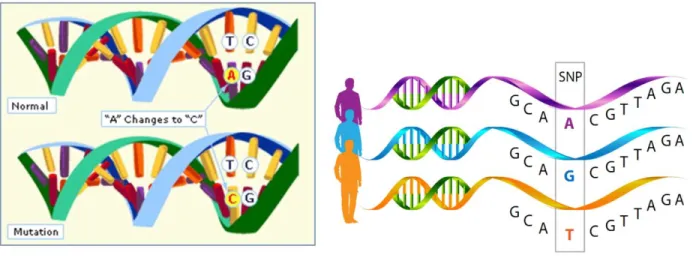
I.8.3 SNP or mutation...31
I.8.4 Phylogenetic tree generation...31
I.8.5 Types of phylogenetic trees...33
I.8.6 Reliability of tree topology...34
Objectives...36
Chapter 1 : Understanding dynamic behaviors of secondary structures...37
1.1 Introduction...37
1.1.1 α- Helices...37
1.1.2 310- Helices...38
1.1.3 π- Helices...38
1.1.4 Prediction of helices from amino acid sequences...39
1.2.1 Data-set preparation...40
1.2.2 Protocol for MD simulations...42
1.2.3 Analysis of local protein conformation...42
1.2.4 Clustering approach...43
1.3 Results and discussions...44
1.3.1 Analyses of protein structures...44
1.3.2 Analyses of molecular dynamics...44
1.3.3 Helical persistence during simulation...45
I.3.3.1 α-helix...45
I.3.3.2 310- helix...46
I.3.3.3 π-helix...47
1.3.4 Impact of sec. structure reassignment on the persistence status...48
1.3.5 Conformational exchanges during simulations...49
1.3.6 k-means Cluster analysis...50
1.3.7 Impact of sec structure reassignment on the exchange rates and dynamics...54
1.4 Conclusions and future perspectives...55
Chapter S1 : Recent advances on polyproline II...58
S1.1 Introduction to polyproline II helices...59
S1.2 Amino acid compositions in PPII helices...60
S1.3 Assignment methods for PPII...61
S1.4 Physiological importance of PPII...64
S1.5 Pathological roles of PPII...66
S1.6 Recent advances in PPII research...67
2.1 Introduction...70
2.1.1 A brief recap...70
2.1.2 Limitations of SSAMs...70
2.1.3 Why Protein Blocks?...71
2.1.4 Previous studies on local flexibility of protein structures...71
2.2 Methods...72
2.2.1 Data set preparation...72
2.2.2 Protocol for MD simulations...72
2.2.3 Analysis of local protein conformation...72
2.2.4 k-means clustering...72
2.3 Results and discussions...73
2.3.1 Analyses of the data set and simulations...73
2.3.2 Dynamics of the non-helical secondary structures...75
2.3.3 Cluster analysis of non-helical states...76
2.3.3.1 Clusters of β-strand...77
2.3.3.2 Clusters of β-turn...78
2.3.3.3 Clusters of bend...79
2.3.4 Overall PB analysis with respect to the initial assignment...80
2.3.5 Cluster analysis of Protein blocks- PB evolution...84
2.3.5.1 Clusters of PB a...84
2.3.5.2 Clusters of PB b...85
2.3.5.3 Clusters of PB f...86
2.3.5.4 Clusters of PB g...87
Chapter 3 : Local protein flexibility in light of physiological structural events...90
3a : Impact of post-translational modifications on protein backbone conformation...92
3a.1 Introduction...92
3a.1.1 Physiological role of Post-Translational Modifications...92
3a.1.2 The PTM code...93
3a.1.3 Effect of PTMs on protein structure...94
3a.1.4 Computational analysis of PTM...94
3a.1.5 PTM-SD...95
3a.2 Methods...97
3a.2.1 Data set preparation...97
3a.2.2 Protein Blocks assignment...99
3a.2.3 Local structure entropy – Neq...100
3a.2.4 Normalization of the B-factor values...101
3a.3 Results and discussions...102
3a.3.1 Impact of PTM on overall protein backbone conformational diversity...102
3a.3.1.1 Neq analysis...102
3a.3.1.2 Analysing structural conformations using PBs....104
3a.3.2 Local backbone diversity in modified structures...105
3a.3.2.1 Neq analysis...105
3a.3.2.1 Statistical significance of differences in local and global flexibility...108
3a.3.3 B-factors and comparison of backbone mobility with and without modifications....109
3a.4 Conclusions and perpectives...111
3b : Characterization of Dual Personality Fragments – DPF...113
3b.1.2 Identification of DPF...116
3b.1.3 Characterization of DPF...117
3b.1.4 Functional importance of DPF...118
3b.1.5 Dynamics in DPF...118
3b.2 Methods...119
3b.2.1 Data set preparation...117
3b.2.2 Feature assignment...117
3b.2.3 Pairwise sequence alignment...118
3b.2.4 Identification of DPF, Order and Disorder regions...120
3b.3 Results and discussions...121
3b.3.1 Data set statistics...112
3b.3.2 Amino acid distributions...122
3b.3.3 Secondary structure distributions...124
3b.3.3.1 Protein blocks distribution...125
3b.3.4 B-factors distribution...127
3b.3.5 Trends in Relative solvent accessibility (rSA) values...128
3b.4 Conclusions and perpectives...130
Chapter 4 : Local structural dynamics in multidomain proteins...134
4.1 Introduction...134
4.1.1 Integrins...135
4.1.1.1 Inside-out signaling...136
4.1.1.2 Outside-in signaling...136
4.1.2 Integrin αIIbβ3...136
4.1.4 Defective expression of integrin αIIbβ3...140 4.1.5 Domains of interest...141 4.1.5.1 Calf-1 domain...143 4.1.5.2 Calf-2 domain...143 4.2 Methods...144 4.2.1 Structural data...144
4.2.1.1 Modeling the missing regions in Calf-2...144
4.2.2 Selected mutations and their structural variants...145
4.2.3 Molecular dynamics...145
4.2.3.1 Trajectory analysis using Protein Blocks...146
4.3 Results and discussions...147
4.3.1 Completing the missing regions in Calf-2 domain...147
4.3.2 Structural analysis of the Calf-1 domain...148
4.3.3 Inherent flexibility in the Calf-1 domain...151
4.3.3.1 Flexible yet rigid: Resolving ability of Neq...151
4.3.4 Comparisons of dynamics between GT variants and WT Calf-1...153
4.3.5 Protein block analysis of WT and variant dynamics...154
4.3.5.1 R724Q...154
4.3.5.2 L653R...156
4.3.5.3 C674R...158
4.3.5.4 Other variants...159
4.4 Conclusions and perspectives...161
Chapter 5 : Protein dynamics in structural assemblies...164
5.1.2 Plasmodium vivax...166
5.1.3 An introduction to DARC...167
5.1.3.1 Sequence of ACKR1 (DARC)...168
5.1.3.2 Physiology of ACKR1 and Chemokine Receptors...170
5.1.3.3 Structure of ACKR1...172
5.1.4 Homology modeling of DARC...173
5.2 Methods...176
5.2.1 Structural template selection...173
5.2.1.1 Template search...176
5.2.1.2 Template selection...177
5.2.1.3 Phylogenetic Analysis for template selection...179
5.2.1.4 Tree generation and visualization...179
5.2.2 Structural Modelling...179
5.2.2.1 Sequence Alignment...179
5.2.2.2 Structural Modelling and assessment...180
5.2.3 Membrane Building...181
5.3 Results and discussions...182
5.3.1 Phylogenetics based selection of the template...182
5.3.2 Structural model for Duffy Antigen / Chemokine Receptor...184
5.3.2.1 T20 test for the selection of the best model...184
5.3.2.2 Structural orientation in the bilayer...185
5.3.3 Comparison with the old computational model of DARC...186
5.3.4 Generation of a mimic RBC bilayer...188
5.4 Conclusions and perspectives...192
Chapter 6 : An evolutionary perspective on Chemokine Receptors...196
6.1 Introduction...196
6.1.1 Chemokines...196
6.1.2 Chemokines and their receptors...199
6.1.3 Chemokine signalling in brief...202
6.1.4 Conservation of microswitches in chemokine receptors...203
6.1.5 Nomenclature of chemokine receptor...204
6.1.5.1 Atypical chemokine receptors...207
6.1.5.1 Virus encoded chemokine receptors (vChemR)...208
6.2 Methods...209
6.2.1 Extraction of homologs and building the dataset...209
6.2.2 Data-set optimization...211
6.2.3 Multiple Sequence Alignment...211
6.2.4 Generating the phylogenetic tree...212
6.2.5 Tree visualization...213
6.3 Results and discussions...213
6.3.1 Composition of the dataset...213
6.3.1.1 Viral chemokine receptors...214
6.3.2 Multiple sequence alignment...214
6.3.3 Tree topology...216
6.3.3.1 Evolutionary placement of ACKR1...217
6.3.3.2 Occurrence of Viral encoded chemokine receptors...218
6.3.6 Structural relatedness between clades...222
6.4 Conclusions and perspectives...228
Conclusive outline......232
I. Introduction...1
I.1 Amino acid structures...2
I.2 Dihedral angles…...3
I.3 Protein structure organization...4
I.4 Beta sheets conformation...5
I.5 Protein family classification...8
I.6 Type of proteins based on cellular environment...10
I.7 Bragg`s law...11
I.8 Workflow of X-ray crystallography...12
I.9 Statistics of EM maps...14
I.10 Simplified view of electron microscopy...15
I.11 A sample CD-spectra for a protein...17
I.12 Growth of sequence space versus structural space...18
I.13 Workflow of PSIPRED...20
I.14 Protein Blocks……...21
I.15 Workflow of Modeller...24
I.16 DNA Substitutions…...30
I.17 Point mutations and SNP...32
Chapter 1 : Understanding dynamic behaviors of secondary structures...37
1.1 Different types of helices...39
1.2 Normalized B-factors, RMSf, and rASA for helices...45
1.3 Normalized B-factors, RMSf, and rASA for whole dataset...46
1.6 Different clusters for 310-helix...52
1.7 Different clusters for π-helix...53
Chapter S1 : Recent advances on polyproline II...58
S1.1 Structural characteristic of three secondary structures...58
S1.2 Orientation and structural organization of different helices...59
S1.3 Ramachandran Map...62
S1.4 Interaction of Nova Protein K homology domain with RNA hairpin...66
S1.5 Year wise publication trends on Polyproline II helices...68
Chapter 2 : Understanding local structure behaviors using Protein Blocks...70
2.1 Distribution of different structural properties in whole dataset...75
2.2 Dynamic exchanges of non-helical DSSP states...76
2.3 Evolution of β-clusters...77
2.4 Evolution of β- turn clusters...78
2.5 Evolution of clusters for bend...80
2.6 CPB in regards to relative solvent accessibility...82
2.7 Exchange rates among different PBs...83
2.8 Evolution of clusters for PB a...85
2.9 Evolution of clusters for PB b...86
2.10 Evolution of clusters for PB f...87
2.11 Evolution of clusters for PB g...88
2.12 Hierarchical clustering of the 5-clusters of each PB...90
Chapter 3 : Local protein flexibility in light of physiological structural events...90
3a : Impact of post-translational modifications on protein backbone conformation...92
3a.3 Using Neq to understand protein backbone flexibility...101
3a.4 Comparison of PTM sites of N-glycosylation and Phosphorylation...103
3a.5 Flexibility profiles of different types of phosphorylation...105
3a.6 N-glycosylation on the Asn141 of human renin endopeptidase...107
3a.7 Local structure comparison of phosphorylation and methylation...108
3a.8 Normalized B-factor distribution for different proteins with and without PTMs...110
3a.9 Impact of methylation on Actin and its ligand binding...111
3b : Characterization of Dual Personality Fragments – DPF...115
3b.1 An example of disorder to order transition...116
3b.2 Schematic flow of DPF, Order and Disorder identification...121
3b.3 Length distribution of DPF across the dataset...122
3b.4 Number of DPF per structure...123
3b.5 Amino acid distributions in Order, DPF, and Disorder...124
3b.6 Secondary structure distribution between DPF and order regions...126
3b.7 Protein Blocks distribution of DPF and order regions...127
3b.8 Normalized B-factor distribution of DPF and Order...128
3b.9 Relative solvent accessibility distribution for DPF and Order...129
Chapter 4 : Local structural dynamics in multidomain proteins...134
4.1 Family schematics of Integrins...135
4.2 Inside-out signaling in Integrins...137
4.3 Closed to open transition of integrin αIIbβ3...139
4.4 Most frequent structures in L33- β3 and V33- β3...142
4.5 Calf-1 and Calf-2 domains demarcation and structural organization...143
4.8 RMSD curves of the WT form of Calf-1 domain...150
4.9 Local rigid conformation in a deformable loop...152
4.10 Ribbon model of Calf-1 domain showing the location of studied variants...153
4.11 Calf-1, RMSf of the different systems...154
4.12 Variant R724Q...155
4.13 The variant L653R…...157
4.14 The variant C674R…...159
4.15 Comparative study of the 𝛥PB values for all WT-variant pairs...160
Chapter 5 : Protein dynamics in structural assemblies...164
5.1 An affair of Plasmodium vivax and ACKR1...165
5.2 Life cycle of a Plasmodium...166
5.3 Disruption of GATA-1 box…...168
5.4 Sequence and structural schema of ACKR1...169
5.5 Chemokine system signalling...171
5.6 Plasmodium vivax and ACKR1 interactions...175
5.7 Phylogenetic placement of ACKR1...183
5.8 Structural model for ACKR1...185
5.9 Structural comparison between old and new models of DARC...187
5.10 Membrane embedded ACKR1 dimer...189
5.11 Dimer interface...191
Chapter 6 : An evolutionary perspective on Chemokine Receptors...196
6.1 Chemokines structure and classification...197
6.2 Schematic representation of chemokines receptors...199
6.5 Chemokines and their receptors... 206 6.6 MSA used for HMM building...210 6.7 MSA used for tree generation...216 6.8 Evolutionary perspective on chemokine receptors...218 6.9 Taxonomic distribution of different chemokine receptor clades...220 6.10 Mammalian contribution to different chemokine receptor sequences...221 6.11 Topology of ACKR1 clade...223 6.12 Tracing ACKR1 evolutionary developements...224
I. Introduction...1
I.1 Characterization of different types of helices found in proteins...4
Chapter 1 : Understanding dynamic behaviors of secondary structures...37
1.1 SCOP ids of the final selected 169 domains...41 1.2 Behaviors of helices...44 1.3 Initial state perseverance of each helix...48 1.4 Exchange rates of helices expressed as percentages...49 1.5 Analysis of different clusters...54
Chapter 2 : Understanding local structure behaviors using Protein Blocks...70
2.1 Frequencies of occurrence of DSSP states during dynamics...73 2.2 Frequencies of occurrence of all PBs during dynamics...74 2.3 CPB- Frequency of PB staying in the initial PB assignment...81
Chapter 3 : Local protein flexibility in light of physiological structural events...90 3a : Impact of post-translational modifications on protein backbone conformation...92
3a.1 The dataset for PTM analysis...97 3a.2 Dataset for phosphorylation sites...98 3a.3 Dataset to analyze local and global impacts of PTMs on 4 proteins...99 3a.4 Statistical tests for the 4 proteins...109
Chapter 5 : Protein dynamics in structural assemblies...164
5.1 Three tier method for filtering template structures...178
Chapter 6 : An evolutionary perspective on Chemokine Receptors...196
INTRODUCTION
I.1 ProteinsProtein are the mediators of information content stored in the DNA and perform myriad of functions inside the cell. From being signalling molecules [1] to enzymes [2] to cellular receptors [3] to forming cytoskeleton [4], they are involved in regulating the cellular function at every step. Genetic information stored in the DNA is transcribed by RNA polymerase into an mRNA transcript which is then used by ribosomes to translate a protein biopolymer. Such sequential transfer of information from DNA to RNA to Protein is known as the central dogma of molecular biology [5]. For a protein to mediate its function, it is required to fold correctly and therefore the relation between protein structure and function is quintessential [6].
I.1.1 Protein sequence
Proteins are made up of amino-acids attached to one another via peptide bonds [7]. Amino acids are the organic molecules containing amine (-NH2) and carboxyl (-COOH) groups as well as an R (side-chain) group which is specific to each amino acid (Fig I.1a). A presence of the amine and carboxyl group states that between pH 2.2 - 9.4, the amino acids contain a negative carboxylate as well as positive ammonium group, hence existing as Zwitterions. Based on the R group, the amino acids can be classified into polar/nonpolar or aliphatic/aromatic or charge/uncharged residues (Fig I.1b). Generally, the non-polar residues form the core of the protein structures while the polar residues are present on the surface to carry out important functions such as catalysis [8].
Figure I.1. Amino acid structure in (a) shows the –NH2, R and –COOH groups and (b) shows the
classification of amino acid based on the nature of R group.
+Source internet, www.stanford.edu/tutorials/biochem/
I.1.2 Structure of proteins
The structure of a protein is dictated by its sequence. Anfinsen, in early 70s conducted a very elegant experiment to prove this characteristic point [9]. The paradigm of sequence-structure-function relationship holds true for majority of the proteins. It states that if two proteins have similar sequences, then it is highly likely that they have similar structures which in turn implies that they should have similar function [10,11]. This underlying principle has been extensively used to predict function for a given protein [12,13]. In order to classify protein structures, it is important to understand the recurring patterns in their 3D arrangement. Ramachandran et al used a model system of two-linked peptide units to identify those conformations which displayed no short-contact between any two atoms [14]. The conformations were selected based on the accessible rotations around N-Cα and C-Cα single bonds called phi (Φ) and psi (Ψ) dihedral angles respectively (Fig I.2).
The values obtained for each accessible Φ and Ψ were plotted as what is famously known today as Ramachandran map. It was observed that the polypeptide backbone can take up certain conformations which are allowed according to the Ramachandran map confirming the occurrence of regular structures in proteins.
Figure I.2. Polypeptide chain in fully extended conformation showing the Φ and Ψ dihedral
angles. The different bond lengths are also shown.
++Source internet: Nelson & Cox, Lehninger Principles of Biochemistry, 4th ed. (2004)
I.2 Protein structure organisation
Protein structures can be organised into four levels of structural hierarchy viz. primary, secondary, tertiary and quaternary (Fig I.3).
I.2.1 Primary structure
An organisation of amino-acids in a linear fashion, next to one another, depicts the primary structure of the protein (Fig I.3). Sequential arrangement of amino acids in a polypeptide chain refers to its primary structure. A protein generally adopts this conformation during the translation process, when the peptide is being polymerized from the ‘P’ site of the ribosome.
I.2.2 Secondary structure
The second level of structural organisation in a protein is defined by secondary structures and is governed by a highly regular, local sub-structural arrangement of polypeptide backbone. Traditionally, these include α-helices and β-sheets (Fig I.3) which are identified by a fixed intra
Figure I.3: Levels of protein structure organisation; Primary, Secondary, Tertiary and
Quaternary structures.
+Source internet, www.ucsf:com/lectures/molecularbiology/proteins
and inter-chain hydrogen-bonding pattern. These secondary structures have a fixed geometry defined by their backbone dihedral angles (Φ and Ψ) and are known to occupy definite location in the Ramachandran map. Example, α-helices occupy the Φ, Ψ position -57, -47 while β-sheets typically occupy position -140, 130. Apart from α-helices, the most prominent helices occurring in the protein, 310 and π-helices are other types of helices that occur in proteins. These types of 3 helices are distinguished by the H-bonding pattern between them. The intra-chain H-bond is formed between i and i+4 residue in the α-helix, between i and i+3 residue in the 310-helix and i and i+5 residue in the π-helix [15,16]. The Φ and Ψ values for these helices are given in Table I.1.
Table I.1. Characteristics of different types of helices found in proteins.
Helix type Phi (Φ) Psi (Ψ) Description
α-helix (R) -57 -47 Right handed α-helix
310-helix -49 -26 Right-handed 310-helix
π-helix -57 -80 Right-handed π-helix
Apart from these, proteins can have also kinks in helices which is often introduced due to a proline residue in the middle of α-helix [17]. Separately, polyproline helices and collagen triple
helix enjoy status of being special cases of secondary structure elements which occur at different Φ, Ψ values than the regular helices and sheets [18,19]. sheets are formed by arrangement of strands in register with each other. They are also classified further into antiparallel and parallel β-sheets depending upon the direction of the strands in register which in turn decides the geometry of H-bond. In an antiparallel arrangement, the consecutive β-strands are in opposite direction to each other such that the N-terminus of one strand is adjacent to the C-terminus of the next (Fig I.4a). This results in a planar H-bond arrangement which deems most suitable for the stability of the β-sheets. The backbone dihedral angles Φ and Ψ for antiparallel sheets are –140°, 135°. On the other hand, parallel β-sheets have the two strands running in same direction making the inter-strand H-bond slightly out-of-plane (Fig I.4b), hence lowering the stability of parallel sheets when compared to antiparallel. The dihedral angles Φ and Ψ are –120°, 115° for the parallel sheets. Strands are rarely long, maximum 15 residues in length and most β-sheets contain less than 6 strands. Side chains from adjacent residues of a strand in a β-sheet are found on opposite sides of the sheet and do not interact with one another. Therefore, like α-helices, β-sheets have the potential for amphiphilicity with one face being polar and the other being non-polar. It has also been noted that parallel sheets are generally buried inside while antiparallel sheets have one side exposed to the solution [20].
Figure I.4. The top and side views of (a) antiparallel β-sheet (b) parallel β-sheet.
Like the kinks in helices, β-sheets are known to have β-bulges which are caused by interruption in the hydrogen bonding [21]. A β-bulge is a region between two consecutive β-type hydrogen bonds which includes two residues (positions 1 and 2) on one strand opposite a single
residue (position x) on the other strand. Two common types of β –bulges are known viz. the “classical” β-bulge and the “G1” β-bulge. The main functional attribute of β-bulges is to accommodate for any single residue insertion or deletion within a β-structure [21].
Besides helices and sheets exist a third kind of structural element called turns which help in reversing the direction of a polypeptide chain. Turns are mainly found on the protein surface and hence contain polar or charged residues and were first identified in protein structures by Venkatachalam [22]. Turns are further classified into α-, β- and γ-turns, out of which β-turns are the most common ones consisting of a sequence of four residues They were defined as linked by a 1-4 (310-type) hydrogen bond between the -C=O of the first residue and the -NH of the fourth residue [20].
α-helices and β-sheets are composed of repetetive units of particular hydrogen bonding patterns as shown in Table I.1 and Fig. I.4. These repetetive units are classified based on their hydrogen bonding and length. A β-bridge is a singelton hydrogen bond observed in isolation with a length of 3 to 4 residues. When multiple bridges exist together, they form a β-sheet [21]. If such hydrogen bonding is missing but the local curvature around the Cα atoms has an angle of 70, it is classified as a bend. A bend is the only secondary structure element whose principle identification is not done by hydrogen bonding pattern [21]. The structural examples of bend and bridges can be seen in Fig. 1.5
I.2.3 Super secondary structures
The secondary structural elements can come together in more than one ways to form some higher order structures. Their structural complexity is smaller than the tertiary structures and denote topological arrangement of helices, sheets and turns. These are called as super-secondary structures and usually occur as small yet functionally important structural motifs. These motifs are generally involved in either biological or structural functions. Some examples include the
helix-turn-helix motif which is known to bind DNA [23], the EF-hand motif known to bind Ca2+ [24] and β-hairpin motif which plays a structural role and connects two antiparallel β-strands [25]. Figure I.3 shows a β-hairpin motif in the secondary structure section.
I.2.4 Tertiary and quaternary level of protein folding
Tertiary structure denotes the 3D arrangement of the secondary structure elements to form a well-folded functional polypeptide (Fig I.3). Tertiary structure is generally defined for a single polypeptide chain where the interior of the folded protein is known as core and is formed by hydrophobic amino acids. The concept of protein domains can be defined at this level. Protein domains are the compact globular modules that are capable of folding and functioning independently of the rest of the protein. Within a protein, different domains can be identified e.g. ligand-binding domain, DNA-binding domain etc.
In many cases, two or more tertiary structures join together to constitute the functional state of a protein. Such organisation of two or more tertiary structures is called quaternary structure of a protein (Fig I.3). Each polypeptide chain in the quaternary structure is termed as a subunit. In other words, quaternary structure can be a homomer, formed from the self-assembly of repeated copies of a single subunit. On the other hand, heteromeric complexes are composed of multiple distinct protein subunits, usually encoded by different genes [26]. Classical example of proteins with similar structure, but one fully functional in tertiary state and the other in quaternary is Myoglobin and Haemoglobin where the former is functional as a single chain while the latter requires association of 4 chains to form a functional molecule [27].
I.3 Structural and functional classification of proteins
Proteins can be classified into various groups depending upon sequence or structural similarity. The classification of proteins becomes important to propose function for a novel protein. One of the ways to classify proteins is to group them into families and superfamilies. A protein family consists of a set of proteins that are evolutionarily related by virtue of similarities in sequence or structure and function. The families can be arranged into hierarchy where the proteins having a common ancestor are grouped into smaller subgroups, indicating more closely related members, called subfamilies. A superfamily consists of different families of proteins where the members within the superfamily are distantly related [28]. A schema of classifying proteins into families is shown in Figure I.5.
Figure I.5: A hypothetical protein family classification showing Family, Superfamily and
Subfamily level hierarchy.
+Source internet. www.ebi.ac.uk
Proteins are grouped into families depending upon similarities in their functional regions, commonly termed as domain. Two classification schemes, one based on similarities between domain sequence and the other based on similarities between domain structures are available. These are Pfam (http://pfam.xfam.org) domain definitions and the SCOP (http://scop.berkeley.edu/) domain definitions.
According to SCOP [29], the protein structures can be classified into following categories depending upon similarities between protein domains:
a) Domain: A part of a protein. For simple proteins, it can be the entire protein
b) Species: The domains in "protein domains" are grouped according to species name
c) Protein domain: Grouping together similar sequences having essentially the same functions
d) Family: It contain proteins with similar sequences signifying homology but typically distinct functions
e) Superfamily: Proteins in a family are grouped together which have at least a distant common ancestor
f) Fold: It groups structurally similar superfamilies
g) Class: Grouping the protein structures mainly on secondary structure content and organization.
Four classes are defined in SCOP - domains containing all α-helices (a.*), domains containing all β-sheets (b.*), domains containing α/β (c.*) and domains containing α+β (mainly segregated, represented as superfamily d.*). SCOP classification also goes beyond ‘c.*’ uptil ‘g.*’ containing different categories of transmembrane proteins. *denotes the sub-family structure after the superfamily a, b, c, d, e, f, and g.
I.4 Protein types based on cellular environment
Protein structures have to correctly fold to perform correct function. Depending on the nature of cellular environment and functional requirements proteins can be either globular, fibrous or membrane proteins.
I.4.1 Globular proteins
Globular proteins are those polypeptide chains that fold into a compact shape. They are the most common protein types. These proteins have a well-defined hydrophobic core such that the apolar residues face towards protein interior while the polar residues face outwards. Functionally these proteins can be enzymes, regulatory proteins, messengers, and transporters etc. Many different folds are associated with globular proteins.
I.4.2 Fibrous proteins
On the other hand, fibrous proteins are generally elongated and are mostly involved in cellular support and structural functions. They are more stable than globular proteins. Some very well characterized fibrous proteins include collagen, actin, myosin, and keratin etc.
I.4.3 Membrane proteins
As the name suggests, membrane proteins are the ones that interact with phospholipid membrane. They can be integral membrane proteins which can be permanently attached to the
[30]. The integral membrane proteins are transmembrane proteins which span across the membranes. It can either be single pass (passing the membrane only once) or multi-pass membrane (passing the membrane more than once) protein. They function mostly as membrane receptors, transport channels, Ion channels, and cell-adhesion and aggregation molecules. Membrane proteins form a separate class in SCOP (e.* to g.*).
An example of globular protein, membrane protein and fibrous protein each is shown in Figure I.6.
Figure I.6: Examples of (a) globular protein – myoglobin (PBDid- 1vxc) (b) membrane protein –
DARC dimer embedded in membrane (modelled in chapter 5) (c) fibrous protein – collagen triple helix (PBDid- 1bkv)
+Source internet, www.rcsb.org/
I.5 Experimental determination of protein structure
Coordinates for 139717 structures have been deposited in the protein data bank (PDB) as of April 29, 2018. Three main experimental methods exist to determine the structure of a protein. These
are X-ray crystallography, nuclear magnetic resonance (NMR) Spectroscopy and cryo-electron microscopy (cryoEM). Out of these, X-ray crystallography has been the method of choice for solving majority of the structures. Though, in the recent years, cryoEM is becoming a popular method to solve the protein structures, especially macromolecular assemblies.
I.5.1 X-ray Crystallography
X-ray crystallography is a technique used to determine the atomic structure of a protein. The technique itself is more than a 100 years old but became a popular method of choice for protein structure determination since 1950s when Sir John Kendrew first solved the structure of sperm whale myoglobin [31]. Since then, 123230 structures solved by crystallography have been deposited in PDB so far. Following structure determination of the lysozyme from bacteriophage T4 (T4 lysozyme) [32], it became a prototype for the study of protein folding and thermodynamics [33].
Briefly, crystallography requires protein crystallisation – a process of forming protein crystals. A unit cell is the crystal repeating unit which defines the smallest group of atoms which has the overall symmetry of a crystal, and from which the entire lattice can be built up by repetition in three dimensions. The protein atoms systematically arrange themselves in three dimension in a unit cell. The protein crystal is then exposed to X-rays causing diffraction according to the Bragg’s law; which states that a constructive interference happens when the condition ‘nλ=2dsinθ’ is satisfied, where d is the distance between two planes, θ is the angle of incidence and λ is the wavelength of X-ray beam (Fig I.7).
Figure I.7. Pictorial representation of Bragg’s law.
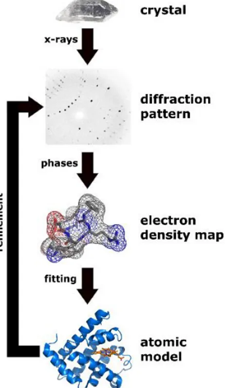
A three-dimensional picture of the electron density within the crystal is produced by measuring the angles and intensities of these diffracted beams. The main challenge in generating the electron density from the diffraction pattern is deciphering the phases which are lost while collecting the diffraction data. This is the notorious phase problem in crystallography, which is the problem of loss of information concerning the phase that can occur when making a physical measurement [34,35]. The phases in crystallography can be obtained by various methods such as molecular replacement (MR), multi-wavelength anomalous diffraction (MAD), multiple isomorphous replacement (MIR) etc. Once the electron density is obtained, the mean positions of the atoms in the crystal as well as the extent of disorder in the structure can be determined. A flow chart for X-ray crystallography is shown in Figure I.8.
Figure I.8. Flowchart showing workflow of X-ray crystallography. A crystal is bombarded with
X-rays to obtain a diffraction pattern. The pattern is then used to generate an electron density map into which atoms are fitted, sometimes based on best guess.
I.5.1.1 Crystal packing defects
Besides, the uncertainty value induced by phase problem there lies another concern with the X-ray technique- The packing of the structure in the crystal. [36]. Although X-ray crystallography gives detailed atomic information about the structure, all the interactions observed in the packed crystals may not be biologically relevant. Many of them may be an artifact of crystal packing and may not be observed in solution. Differentiating the true interactions from such non-specific interaction may become a daunting task [37,38]. An analysis of general interface properties has revealed some features to distinguish specific vs non-specific interactions within crystals [39,40]. These properties include interface area, composition of the interface, spatial distribution of the interface residues, secondary structure, core interface conservation and the space group to which they belong. A recent study has shown that many of these properties are indistinguishable for the specific and non-specific interactions [41] and hence one has to be cautious while analysing protein-protein contacts obtained from the crystal structures.
I.5.2 Nuclear Magnetic Resonance- NMR
NMR is the second most common method to determine protein structures. Most NMR structures consist of a single type of polypeptide chain and a majority of the structures solved using NMR are monomers [42]. This is because smaller proteins are easily characterized using NMR than the larger proteins and hence the proteins that tend to exist as huge oligomers are not amenable to structure determination using NMR. It has been shown that since 2005, the number of structures determined using NMR in PDB has sharply decreased showing a fall in the popularity of the method [42]. Even though NMR spectroscopy is usually limited to proteins smaller than 35 kDa, it is often the only method to study the conformational heterogeneity and intrinsically disordered nature of proteins.
NMR exploits the quantum mechanical properties of the central core ("nucleus") of the atom. These properties depend on the local environment of the molecules and their measurement provides a map of how the atoms are chemically linked, how close are they in space, and how rapidly they move with respect to each other. Principle behind obtaining NMR spectra is that each
distinct nucleus in a protein experiences a distinct electronic environment and thus has a distinct chemical shift by which it can be recognized. A resonance assignment is obtained for the protein to find out the chemical shift corresponding to each atom. To perform structure calculations, a number of experimentally determined restraints are generated like distance restraints and angle restraints. These restraints are used as an input to generate multiple structures satisfying these restraints. Hence, NMR generates an ensemble of structures while X-ray crystallography provides one structure which generally is a space and time-averaged structural snapshot.
I.5.3 Cryo-electron Microscopy
Though X-ray crystallography is considered as the gold standard for providing atomic resolution structures, it suffers from the drawback of providing a static snapshot which may be far from the physiological structure. Also, many proteins resist crystal formation and a lot of time and effort has to be invested to solve the structure using X-ray crystallography. NMR on the other hand, though being capable of elucidating dynamics information is limited by the size considerations. Hence, cryoEM can provide solutions to these limitations such that it can be used for bigger protein complexes and can image complexes in their physiological environment [43]. Although the use of cryoEM technique has been limited to medium to low (5-15 Å) resolution range yet structures with resolution better that 3 Å are getting published thus making the technique tractable [44]. CryoEM is becoming the most sought after technique to extract structural information about the macromolecular complexes not amenable to either X-ray or NMR. After procuring a density map, the most important task is to obtain a high confident pseudo-atomic model for the same. The structures to be fitted into the electron density map can either be the crystal structures of a subcomponent or can be a homology modeled structure. If the density map resolution is better than 4 Å, de-novo modeling can be used to calculate the pseudo-atomic model.
CryoEM is a type of Transmission Electron Microscopy (TEM), in which the sample is studied at cryogenic temperatures. The information obtained is invaluable in understanding the macromolecular assembly at physiological conditions. CryoEM techniques can be classified into three types: a) Electron Crystallography, b) Single particle analysis, and c) Cryo-electron tomography. Out of these single-particle analysis or Single particle cryoEM is emerging as a technique of choice to determine 3D structure of proteins with an increasingly advancing electron
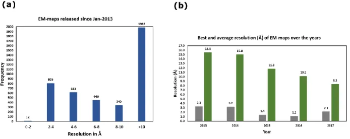
beams, detectors and ability to analyse isolated complexes (“Single particles”) under native conditions [45]. Its emergence can be judged from the number of EM maps being released every year as well as the improvement in their resolution ranges (Fig I.9).
Figure I.9. Statistics of EM maps and their resolution since 2013. (a) shows the frequency of
occurrence of various resolutions of EM maps and (b) shows the best and average resolutions over the years. The worst resolution has been clipped to 30Å for this plot.
+Source internet, www.emdb.org/
The basic principle behind electron microscopy is the deflection of electrons in an electromagnetic field. An EM consists of an electron source, a series of lenses, and an image detecting system, which currently are high-end digital cameras [46]. As the electrons from the source hit the condenser lens, they are converged and fall on the object as a parallel beam. The aperture at the back focal plane of objective lens filters out the electrons scattered at very high angles, hence preventing them from reaching the image plane. Image magnification is provided by the objective lens and the projector lens. Once a good quality image is obtained, next task is to generate 3D reconstruction of the 2D projections of the objects using the phase information present in the image itself. The next important task after obtaining 3D electron density map is to calculate the pseudo-atomic model for the structure in question. Depending on the resolution, this can be achieved either through de-novo model building or through rigid body fitting or flexible fitting of
predicted models / structures from other techniques. A simplified view of the electron microscope is given in Figure I.10.
Figure I.10: A simplified view of the electron microscope.
+
Taken from [46]
I.5.4 Circular Dichroism spectroscopy
Another popular technique to determine the secondary structure content of the proteins is the Circular Dichroism (CD) spectroscopy which is based on the principle of the differential absorption of the left and right-handed circular polarised light. This technique is a routine to precisely estimate the secondary structure content of the protein and confirm their proper folding under the experimental setup. A typical CD spectral profile for different secondary structure looks like Figure I.11.
Figure I.11. A sample CD-spectra for a protein. The profiles for different secondary structures
are shown in different colours.
+Sourceinternet,www.fbs.leeds.ac.uk/facilities/cd/
I.6 Computational Structural Biology: In silico techniques for protein structures
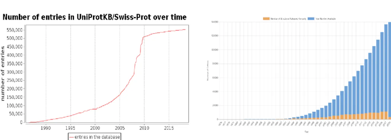
It takes a considerable amount of time and effort to experimentally determine the three-dimensional structure of proteins using any of the above mentioned techniques. It sometimes takes from months to years to obtain a protein crystal which can successfully diffract. Though cryoEM circumvents the need of getting crystals, the technique is more amenable to the proteins with higher molecular weight. Moreover, the growth in structural space for proteins does not match up to the speed with which sequence space is growing (Fig I.12).
Hence, it becomes increasingly important to resort to the computational methods to predict three-dimensional structure of a given protein. The history of theoretically predicting the structural elements dates back to 1970s when Chou and Fasman calculated the propensities of amino acids in α-helices, β-sheets and turns [47]. Since then various methods have been developed to predict the secondary structures from the sequence [48–50]. Protein secondary structure prediction refers to the prediction of the conformational state of each amino acid residue of a protein sequence as one of the three possible states, namely, helices, strands, or coils, denoted as H, E, and C, respectively.
Another important application of computational methods is their ability to predict tertiary structure of proteins. Three main approaches are employed in computational 3D prediction are: homology modelling, threading, and ab-initio prediction. The first two are knowledge-based methods; they predict protein structures based on knowledge of existing protein structural
information in databases. Homology modelling builds an atomic model based on an experimentally determined structure that is closely related at the sequence level. Threading identifies proteins that are structurally similar, with or without detectable sequence similarities. The ab initio approach requires molecular simulations to predict structures based on physicochemical principles governing protein folding without the use of structural templates. There are meta-servers that combine fold recognition and homology modelling to model a structure based on multiple templates matching different folds.
Figure I.12. Growth of sequence space vis-à-vis the structural space. (a) shows the number of
sequences deposited in Uniprot since 1990 (Taken from Uniprot) (b) shows the number of structures deposited in PDB over the years
+Source internet www.rcsb.org
I.6.1 Secondary structure assignment
Given their fundamental importance in protein structures, it is important to define and characterize secondary structure elements for a given protein structure. Various standard methods are available for this purpose. Several assignment methods can be used like, DSSP [51], STRIDE [52] and predefined libraries of secondary structure can also be used.
I.6.1.1 DSSP – Define secondary structure of proteins
The DSSP algorithm is a standard method for assigning secondary structure to the amino acids of a protein using the coordinates of the structure. The DSSP program was designed by Wolfgang Kabsch and Chris Sander. It identifies the intra-backbone hydrogen bonds of the protein using a purely electrostatic definition. A hydrogen bond is identified
if E in the following equation is less than -0.5 kcal/mol. Based on the identified hydrogen bonds, eight types of secondary structure are assigned. These eight types are usually grouped into three larger classes: helix (G, H and I), strand (E and B) and loop (S, T, and C, where C sometimes is represented also as blank space).
I.6.1.2 STRIDE - STRuctural Identification
STRIDE is also a secondary structure assignment tool like DSSP but instead of using only the hydrogen bond potential, it also includes dihedral angle potentials to define secondary structures within a protein. Hence, its criteria for defining individual secondary structures are more complex than those of DSSP. The STRIDE energy function contains a hydrogen-bond term containing a Lennard-Jones-like 8-6 distance-dependent potential and two angular dependence factors reflecting the planarity of the optimized hydrogen bond geometry. The criteria for individual secondary structural elements, which are divided into the same groups as those reported by DSSP, also contain statistical probability values derived from empirical examinations of solved structures. There have been comparisons between DSSP and STRIDE since their inception. It has been shown than DSSP and STRIDE agree for 95% of the cases [53]. I should be noted that it has been shown than both DSSP and STRIDE under-represent π-helix [54].
I.6.2 Secondary structure prediction
The prediction of secondary structures is based on the regular arrangement of amino acids in the secondary structures which are stabilized by hydrogen bonding patterns. The structural regularity serves the foundation for these prediction algorithms. Protein secondary structure prediction with high accuracy is not a trivial task. It has remained a very difficult problem for decades. Specifically, because protein secondary structure elements are context dependent. The formation of α-helices is determined by short-range interactions, whereas the formation of β-strands is strongly influenced by long-range interactions. Prediction for long-range interactions is theoretically difficult. Albeit, after more than three decades of effort, prediction accuracies have only been improved from about 50% to about 82%. There are many methods available for secondary structure prediction. Out of these PSIPRED is the most popular one [49].
PSIPRED (http://bioinf.cs.ucl.ac.uk/psipred/) is a web-based program that predicts protein secondary structures using a combination of evolutionary information and neural networks. PSIPRED incorporates two feed-forward neural networks which performs an analysis on output obtained from PSI-BLAST. A profile is extracted from the multiple sequence alignment generated from three rounds of the PSI-BLAST. This profile is then used as input for a neural network prediction. To achieve higher accuracy, a unique filtering algorithm is implemented to filter out unrelated PSI-BLAST hits during profile construction. A schematic of PSIPRED is shown in Figure I.13.
Figure I.13. Workflow of PSIPRED.
+Taken from [42].
I.6.3 Protein Blocks: A comprehensive structural alphabet
A structural alphabet (SA) is a library of N structural prototypes (the letters). Each prototype is representative of a backbone local structure of l-residues length. The combination of those structural prototypes is assumed to approximate any given protein structure. One of the most developed and comprehensive SA is the Protein Blocks (PBs) [53].
PBs are a structural alphabet composed of a set of 16 local prototypes each of 5 residues length, labeled from a to p (see Fig I.14 Bottom). They are described as series of eight Φ, Ψ dihedral angles. An unsupervised classifier similar to Kohonen Maps [55,56] and Hidden Markov Models [57] was used to define PBs. Therefore, they approximate all the local regions of a protein structure with an average RMSD of 0.41 Å [58]. The PBs m and d can be roughly described as prototypes for the central region of α-helix and β-strand, respectively. PBs a-c primarily represent the N-cap of β-strand while e and f correspond to C-caps; PBs g - j are specific to coils, PBs k and
l correspond to N cap of α-helix while PBs n - p to C-cap.
Figure I.14: Protein blocks. Top row depicts the 5 residue long prototype. Bottom row shows the 16 protein blocks along with their respective secondary structure approximations.
+Adapted from [53] and [58].
PB Assignment: For each “nth” position of the structure, 8 dihedrals ψ (n − 2), φ (n − 1), ψ
(n − 1), φ (n), ψ (n), φ (n + 1), ψ (n + 1), φ (n + 2) are compared to the dihedrals of each of the 16 PBs. The comparison is made by a least squares approach to match the RMSDA criteria (Root
𝑅𝑀𝑆𝐷𝐴 (𝑉1, 𝑉2) = √ 1 2(𝑀−1) ∑
𝑀−1
𝑖=1 [𝜓𝑖(𝑉1) − 𝜓𝑖(𝑉2)]2+ [𝜙𝑖+1(𝑉1) − 𝜙𝑖+1(𝑉2)]2
where, V1 is the 8 dihedrals vector extracted from the 5 residues long window; V2 is the 8
dihedrals vector corresponding to the compared PBs. PB, which gets lowest RMSDA is chosen as
the representing conformation observed in the window.
Applications: PBs have been used to address various problems including, protein
superimposition [60,61], general analyses of flexibility [62,63] and prediction of structure and flexibility [64–67] and protein binding sites, and structural analysis of β-bulges [68]. PBs can be assigned to a given structure or an ensemble with valid coordinates using PBxplore [69]. The structural analysis of different structural dataset is assisted by two statistical measures derived from the assigned PBs.
Neq: Quantification of the structural flexibility at a given position n, can be obtained by
calculating the average number of PBs across a set of conformers at position n. This is called the “equivalent number” of PBs or Neq. Neq is based on a statistical metric similar to Shannon entropy [53]. It is calculated as:
𝑁𝑒𝑞 = 𝑒𝑥𝑝 (− ∑ 16
𝑖=1
𝑓𝑥. 𝑙𝑛(𝑓𝑥))
where fx is the frequency of PB ‘x’. The value of x can be any PB from a to p. An Neq value of 1 will indicate that only one type of PB is observed at position n while Neq value of 16 will denote a random and propotional (1:16) distribution.
I.6.4 Tertiary structure prediction
The tertiary structure of the proteins is predicted either using ab-initio methods or based on a template identified through homology. The latter is the more common, reliable, less time-consuming method and is based on the paradigm that similar sequences have similar structures and hence similar functions [10], [11]. Homology modelling starts with identification of a suitable template which shares homologous relationship with the sequence of interest. Using elegant
computational algorithms, the coordinates of the backbone of the template are copied to the query and the side chains are optimised. Modeller is the most popular program to perform molecular modelling and is described in brief herein [70].
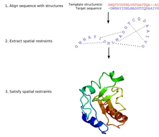
I.6.4.1 Modeller
Modeller is a computer program that models three-dimensional structures of proteins and their assemblies by satisfaction of spatial restraints (Fig I.15). The initial step before starting the modelling procedure is to identify a suitable template. This forms the foundation for rest of the modelling process. The template selection involves searching for a homologous structure in PDB using either BLAST [71] or any other fold recognition tool such as Phyre2 [72] or HHpred [73]. Generally, the structures with sequence identity greater than 30% are considered safely as homologous to the query protein. Once the structure of suitable confidence is identified as a template, an alignment is performed between the query and the template. This can be achieved either using scripts from Modeller or using a suitable alignment tool. This alignment, in PIR format, is the input to the Modeller program. From its alignment with template 3D structures, Cα- Cα distances, hydrogen bonds and dihedral angle restraints for the target sequence are calculated by Modeller. The form of these restraints has been obtained from a systematic statistical analysis of the relationships between many pairs of homologous structures [74]. The spatial restraints are obtained empirically, from a database of protein structure alignments. These restraints are expressed as probability density functions (pdfs) for the features to be restrained. For example, the probabilities for main-chain conformation of an equivalent residue in a related protein are expressed as a function of the local similarity between the two sequences. A smoothening procedure has been employed in the derivation of these relationships to minimise the problem of sparse database. Next, these spatial restraints and Charmm energy terms enforcing proper stereochemistry are combined into an objective function [75]. The output is a 3D model for the target sequence containing all main-chain and side-chain non-hydrogen atoms which ensures a minimal deviation from the input restraints. The final model is then optimised using variable target function methods employing methods of conjugate gradients and molecular dynamics with simulated annealing. Several slightly different models can be calculated by varying the initial