IMPROVEMENT AND INTEGRATION OF COUNTING-BASED SEARCH HEURISTICS IN CONSTRAINT PROGRAMMING
SAMUEL GAGNON
DÉPARTEMENT DE GÉNIE INFORMATIQUE ET GÉNIE LOGICIEL ÉCOLE POLYTECHNIQUE DE MONTRÉAL
MÉMOIRE PRÉSENTÉ EN VUE DE L’OBTENTION DU DIPLÔME DE MAÎTRISE ÈS SCIENCES APPLIQUÉES
(GÉNIE INFORMATIQUE) MAI 2018
c
ÉCOLE POLYTECHNIQUE DE MONTRÉAL
Ce mémoire intitulé :
IMPROVEMENT AND INTEGRATION OF COUNTING-BASED SEARCH HEURISTICS IN CONSTRAINT PROGRAMMING
présenté par: GAGNON Samuel
en vue de l’obtention du diplôme de: Maîtrise ès sciences appliquées a été dûment accepté par le jury d’examen constitué de:
M. DAGENAIS Michel, Ph. D., président
M. PESANT Gilles, Ph. D., membre et directeur de recherche M. ROUSSEAU Louis-Martin, Ph. D., membre
DEDICATION
To my parents, for which education has always been an important value. . .
À mes parents, pour qui l’éducation a toujours été une valeur importante. . .
ACKNOWLEDGEMENTS
I would like to thank the Natural Sciences and Engineering Research Council of Canada for their financial support. I would also like to thank Gilles, my supervisor, which patiently guided me throughout my master’s degree by encouraging me to try out my ideas.
J’aimerais remercier le Conseil de recherches en sciences naturelles et en génie du Canada d’avoir fourni un support financier à notre recherche. J’aimerais également remercier Gilles, mon directeur de recherche, qui m’a patiemment guidé tout au long de ma maîtrise en m’encourageant à essayer mes idées.
RÉSUMÉ
Ce mémoire s’intéresse à la programmation par contraintes, un paradigme pour résoudre des problèmes combinatoires. Pour la plupart des problèmes, trouver une solution n’est pas possible si on se limite à des mécanismes d’inférence logique; l’exploration d’un espace des solutions à l’aide d’heuristiques de recherche est nécessaire. Des nombreuses heuristiques existantes, les heuristiques de branchement basées sur le dénombrement seront au centre de ce mémoire. Cette approche repose sur l’utilisation d’algorithmes pour estimer le nombre de solutions des contraintes individuelles d’un problème de satisfaction de contraintes.
Notre contribution se résume principalement à l’amélioration de deux algorithmes de dénom-brement pour les contraintes alldifferent et spanningTree; ces contraintes peuvent exprimer de nombreux problèmes de satisfaction, et sont par le fait même essentielles à nos heuristiques de branchement.
Notre travail fait également l’objet d’une contribution à un solveur de programmation par contraintes open-source. Ainsi, l’ensemble de ce mémoire est motivé par cette considération pratique; nos algorithmes doivent être accessibles et performants.
Finalement, nous explorons deux techniques applicables à l’ensemble de nos heuristiques: une technique qui réutilise des calculs précédemment faits dans l’arbre de recherche ainsi qu’une manière d’apprendre de nouvelles heuristiques de branchement pour un problème.
ABSTRACT
This thesis concerns constraint programming, a paradigm for solving combinatorial problems. The focus is on the mechanism involved in making hypotheses and exploring the solution space towards satisfying solutions: search heuristics. Of interest to us is a specific family called counting-based search, an approach that uses algorithms to estimate the number of solutions of individual constraints in constraint satisfaction problems to guide search.
The improvements of two existing counting algorithms and the integration of counting-based search in a constraint programming solver are the two main contributions of this thesis. The first counting algorithm concerns the alldifferent constraint; the second one, the spanningTree constraint. Both constraints are useful for expressing many constraint satisfaction problems and thus are essential for counting-based search.
Practical matters are also central to this work; we integrated counting-based search in an open-source constraint programming solver called Gecode. In doing so, we bring this family of search heuristics to a wider audience; everything in this thesis is built upon this contribution. Lastly, we also look at more general improvements to counting-based search with a method for trading computation time for accuracy, and a method for learning new counting-based search heuristics from past experiments.
TABLE OF CONTENTS
DEDICATION . . . iii
ACKNOWLEDGEMENTS . . . iv
RÉSUMÉ . . . v
ABSTRACT . . . vi
TABLE OF CONTENTS . . . vii
LIST OF TABLES . . . x
LIST OF FIGURES . . . xi
LIST OF ANNEXES . . . xiii
CHAPTER 1 INTRODUCTION . . . 1
1.1 CSP Formulation of the Magic Square Problem . . . 1
1.1.1 Inference . . . 3
1.1.2 Search . . . 4
1.1.3 Consistency Levels for Constraints . . . 6
1.2 Problem Under Study . . . 7
CHAPTER 2 LITERATURE REVIEW . . . 9
2.1 Survey of Generic Branching Heuristics . . . 9
2.1.1 Fail First Principle . . . 9
2.1.2 Impact-Based Search . . . 10
2.1.3 The Weighted-Degree Heuristic . . . 10
2.1.4 Activity-Based Search . . . 10
2.1.5 Counting-Based Search . . . 11
2.2 Effort for Reducing Computation in the Search Tree . . . 13
2.3 Adaptive Branching Heuristics . . . 14
CHAPTER 3 ACCELERATING COUNTING-BASED SEARCH . . . 15
3.1 Alldifferent Constraints . . . 15
3.1.2 Computing Maximum Solution Densities Only . . . 17
3.2 Spanning Tree Constraints . . . 18
3.2.1 Faster Specialized Matrix Inversion . . . 19
3.2.2 Inverting Smaller Matrices Through Graph Contraction . . . 19
3.3 Avoiding Systematic Recomputation . . . 20
CHAPTER 4 PRACTICAL IMPLEMENTATION OF COUNTING-BASED SEARCH IN GECODE . . . 22
4.1 Basic Notions in Gecode . . . 22
4.1.1 Main Loop in Gecode . . . 23
4.1.2 Creation of the Model . . . 23
4.1.3 Creation of the Search Strategy . . . 25
4.1.4 Solving the Problem . . . 26
4.2 Basic Structure for Supporting Counting-Based Search in Gecode . . . 26
4.2.1 Unique IDs for Variables . . . 28
4.2.2 Methods for Mapping Domains to their Original Values . . . 29
4.2.3 Computing Solution Distributions for Propagators . . . 30
4.2.4 Accessing Variable Cardinalities Sum in Propagators . . . 30
4.3 Counting Algorithms . . . 31
4.4 Creating a Brancher Using Counting-Based Search . . . 31
CHAPTER 5 EMPIRICAL EVALUATION . . . 33
5.1 Impact of our Contributions . . . 33
5.1.1 Acceleration of alldifferent . . . 33
5.1.2 Acceleration of spanningTree . . . 34
5.1.3 Avoiding Systematic Recomputation . . . 35
5.2 Benchmarking our Implementation in Gecode . . . 36
5.2.1 Magic Square . . . 37
5.2.2 Quasigroup Completion with Holes Problem . . . 38
5.2.3 Langford Number Problem . . . 39
CHAPTER 6 BRANCHING HEURISTIC CREATION USING A LOGISTIC REGRES-SION . . . 41
6.1 Problem Definition . . . 41
6.2 Experiment . . . 43
6.2.1 First Logistic Function . . . 43
CHAPTER 7 CONCLUSION . . . 47
7.1 Discussion of Contributions . . . 47
7.2 Limits and Constraints . . . 48
7.3 Future Research . . . 49
REFERENCES . . . 50
LIST OF TABLES
Table 6.1 Offline database with densities for multiple single solution instances of the same problem. . . 42 Table 6.2 Logistic function combining h2∧ h5 against both branching heuristic. 44
LIST OF FIGURES
Figure 1.1 Partially filled magic square instance . . . 2
Figure 1.2 Model for magic square in Fig 1.1 . . . 3
Figure 1.3 P . . . 4
Figure 1.4 Solution space splitting . . . 4
Figure 1.5 P ∧ h1 . . . 5
Figure 1.6 Solution space split after h2 . . . 5
Figure 1.7 P ∧ h1∧ h2 . . . 6
Figure 1.8 P ∧ h1∧ h2∧ h3 . . . 6
Figure 1.9 P ∧ h1 . . . 7
Figure 3.1 Incidence matrix for alldifferent(x1, x2, x3) with D1 = {1, 2}, D2 = {2, 3} and D3 = {1, 3} . . . . 15
Figure 3.2 Graph and its Laplacian matrix with γ = 2, meaning we can get every edge density by inverting two submatrices, e.g. L1 (with inverse M1 shown) and L3 . . . . 19
Figure 3.3 Contraction following assignments e(1, 2) = 1 and e(1, 4) = 1, with 1 as the representative vertex in connected component {1, 2, 4} . . . . . 20
Figure 3.4 Connected component {1, 2, 4} as a single vertex . . . . 20
Figure 4.1 Gecode model for the magic square problem in Fig. 1.2 . . . 24
Figure 4.2 Variables for model in Fig. 4.1 . . . 24
Figure 4.3 Constraints for model in Fig. 4.1 . . . 25
Figure 4.4 Brancher for model in Fig. 4.1 . . . 26
Figure 4.5 Modeling the magic square with a custom brancher using Gecode . . 28
Figure 4.6 Principal components in relation with CBSBrancher . . . 32
Figure 5.1 Percentage of Quasigroup Completion instances solved w.r.t. time and number of failures . . . 34
Figure 5.2 Percentage of Hamiltonian Path instances solved w.r.t. time and num-ber of failures with a 5 minute cutoff . . . 35
Figure 5.3 The effect of different recomputation ratios for the Quasigroup Com-pletion Problem, using the same instances as in Section 5.1.1 . . . 36
Figure 5.4 The effect of different recomputation ratios for Hamiltonian Path Prob-lem, using same instances as in Section 5.1.2 . . . 36
Figure 5.5 Percentage of magic square instances solved w.r.t. time and number of failures . . . 38
Figure 5.6 Percentage of latin square instances solved w.r.t. time and number of
failures . . . 39
Figure 5.7 Percentage of langford instances solved w.r.t. time and number of failures 40 Figure 6.1 Logistic function as a new branching heuristic . . . 43
Figure 6.2 Rotation of t(h2, h3) around the mean value of h2 and h3 . . . 45
Figure 6.3 Landscape of performance for 90 logistic functions . . . 46
Figure A.1 Generic template for a counting algorithm in solndistrib . . . 57
Figure A.2 Generic template for domainsizesum . . . 58 Figure B.1 Good and bad branching choices according to each branching heuristic 59
LIST OF ANNEXES
Annexe A NOTES ABOUT COUNTING ALGORITHMS IMPLEMENTATION 55
CHAPTER 1 INTRODUCTION
Constraint programming (CP) is a declarative paradigm that has proven useful for solving large combinatorial problems, particularly in the areas of scheduling and planning. Appearing in the eighties, this approach was influenced by various fields such as Artificial Intelligence, Programming Languages, Symbolic Computing and Computational Logic [Barták (2018)]. Constraint programming can be seen as a competitor to other mathematical programming approaches such as linear programming (LP) or integer programming (IP). As constraint programming is more niche, one could ask why it is worth using instead of other paradigms. One of the biggest selling points of CP is that the formulation of a problem is simple and straightforward; models in constraint programming are described by high level concepts that are close to the original problem formulation. With the Constraint Satisfaction Problem (CSP) as one of the main abstractions, modeling is done by expressing constraints on vari-ables. This is in contrast with other mathematical programming approaches where con-straints are translated to mathematical equations. Reasoning about the model and designing search heuristics is much simpler as a result.
Constraint programming solvers offer a catalog that goes from binary inequalities to complex constraints like bin packing and Hamiltonian path. Typically, these global constraints can be reformulated with several simpler constraints (like we would do in LP/IP). However, global constraints are able to solve problems faster because they encapsulate the semantic of bigger pieces in the problem; thus enabling models to be very precise [van Hoeve and Katriel]. In a constraint programming solver, a CSP is solved by giving a model of the problem and a search strategy, thus offering a declarative programming framework: the user describes the structure of the problem without specifying how to solve it. Behind the scenes, the solver combines various algorithms to solve the problem according to the specifications — its model and the search strategy.
In the next sections, basic notions in constraint programming will be introduced by looking at an example: the Magic Square Problem.
1.1 CSP Formulation of the Magic Square Problem
A CSP is formally described by the following tuple:
where
• X = {x1, . . . , xn} is a finite set of variables.
• D = {D1, . . . , Dn} is a finite set of domains such that xi ∈ Di.
• C = {C1, . . . , Ct} is a finite set of constraints. A constraint Ci on variables x1, . . . , xk
is a relation that restricts the Cartesian product of its variables to a subset Ci ⊆
D1× · · · × Dk.
A solution to P is an assignment that satisfies all constraints. As previously said, the first step in CP is to give a description of the problem.
16 . . .
. 10 . .
. . 7 .
. . . .
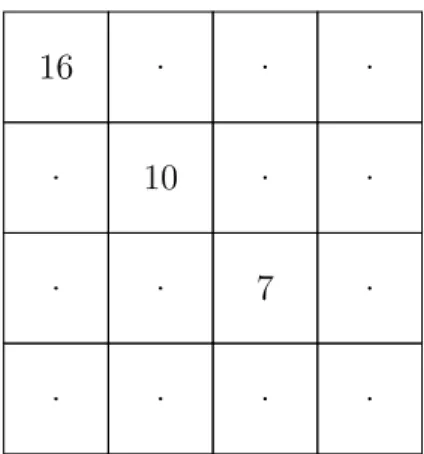
Figure 1.1 Partially filled magic square instance
Let’s take the example of the magic square instance shown in Fig. 1.1. An order n magic square is a n by n matrix containing the numbers 1 to n2, with each row, column and main
diagonal equal to n(n2+ 1)/2 (#19 in CSPLib [Walsh (2018)]). The magic square in Fig. 1.1
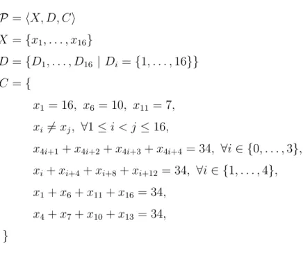
P = hX, D, Ci X = {x1, . . . , x16} D = {D1, . . . , D16 | Di = {1, . . . , 16}} C = { x1 = 16, x6 = 10, x11= 7, xi 6= xj, ∀1 ≤ i < j ≤ 16,
x4i+1+ x4i+2+ x4i+3+ x4i+4 = 34, ∀i ∈ {0, . . . , 3},
xi+ xi+4+ xi+8+ xi+12 = 34, ∀i ∈ {1, . . . , 4},
x1+ x6+ x11+ x16= 34,
x4+ x7+ x10+ x13= 34,
}
Figure 1.2 Model for magic square in Fig 1.1
1.1.1 Inference
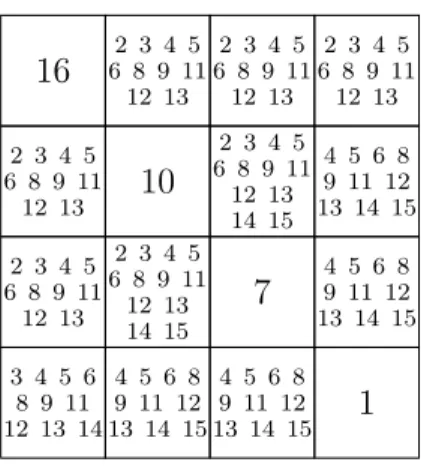
Given the previous CSP, the next task is to do constraint propagation on the given problem to obtain local consistency for all constraints (thus obtaining what we call a stable state). In other words, we deduce everything we can from the CSP formulation of our problem. For example, we can deduce that x16= 1 because the sum of the diagonals must be equal to 34.
For a constraint, propagation is the process of filtering incoherent values from the domain of its variables.
Obtaining a stable state is done by scheduling all constraints for propagation. Each time a constraint propagates, it may reschedule another one by modifying a variable in its scope. Eventually, we obtain a stable state when this process finishes and all constraints have lo-cal consistency. In a finite domain constraint programming solver, this process will always terminate because each new iteration has to prune variable domains.
16 6 8 9 112 3 4 5 12 13 2 3 4 5 6 8 9 11 12 13 2 3 4 5 6 8 9 11 12 13 2 3 4 5 6 8 9 11 12 13 10 2 3 4 5 6 8 9 11 12 13 14 15 4 5 6 8 9 11 12 13 14 15 2 3 4 5 6 8 9 11 12 13 2 3 4 5 6 8 9 11 12 13 14 15 7 4 5 6 89 11 12 13 14 15 3 4 5 6 8 9 11 12 13 14 4 5 6 8 9 11 12 13 14 15 4 5 6 8 9 11 12 13 14 15 1 Figure 1.3 P
Here, we could ask why 14 ∈ D13: there is no valid assignment satisfying 16+x5+x9+14 = 34,
as x5 and x9 should both be equal to 2, thus violating the alldifferent constraint. The
key observation is that both constraints are locally consistent, the alldifferent constraint is not involved for evaluating supporting solutions of other linear constraints.
1.1.2 Search
Constraint propagation was not sufficient for finding a valid solution to our problem; we still have to find a valid assignment for 12 variables. To this end, we need the second component of the solver: a search strategy. The search strategy is used to make hypotheses to prune the search space when no more constraint propagation is possible. A valid search strategy for our problem could be as simple as:
• Select the variable xi with the smallest domain
• Select the smallest value v ∈ Di
• Split the solution space as P ∧ (xi = v) ∪ P ∧ (xi 6= v)
This strategy splits P into two valid CSPs (with h1 : xi = v):
P
P ∧ h1 P ∧ h1
If we apply this search strategy to our example, we have x5 with a cardinality of 10 and a
minimum value of 2, giving us the hypothesis h1 : x5 = 2. The component of the search
strategy that gives hypotheses is called a branching heuristic. After constraint propagation, we get the state shown in Fig. 1.5.
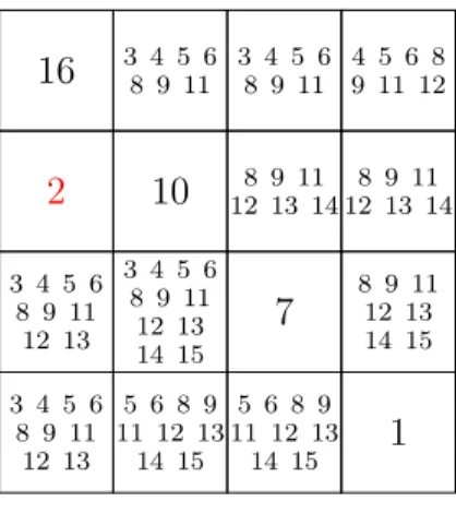
16 3 4 5 68 9 11 3 4 5 68 9 11 4 5 6 89 11 12 2 10 12 13 148 9 11 12 13 148 9 11 3 4 5 6 8 9 11 12 13 3 4 5 6 8 9 11 12 13 14 15 7 8 9 1112 13 14 15 3 4 5 6 8 9 11 12 13 5 6 8 9 11 12 13 14 15 5 6 8 9 11 12 13 14 15 1 Figure 1.5 P ∧ h1
However, we still haven’t found a solution. If we use our branching heuristic again, we get a second hypothesis h2 : x7 = 8 that leads, after constraint propagation, to the state in
Fig. 1.7.
P
P ∧ h1 P ∧ h1
P ∧ h1∧ h2 P ∧ h1∧ h2
16 6 9 4 5 6 4 5 6
2 10 8 14
3 4 5 9 11 7 13 15
11 12 13 5 6 9 13 15 1
Figure 1.7 P ∧ h1∧ h2
Finally, a third hypothesis h3 : x2 = 6 will lead us to a failed state. In other words,
finding a solution is now impossible as the maximum sum we can obtain in the first row is 16 + 6 + 5 + 5 = 31, which is lower than 34. This means that our sequence of hypotheses (shown in red) is incorrect.
16 6 4 5 4 5
2 10 8 14
3 4 5 9 11 7 13 15
11 12 13 5 9 13 15 1
Figure 1.8 P ∧ h1∧ h2∧ h3
If we continue the exploration of this implicit tree in a depth-first search fashion, we will eventually find a solution for this particular instance.
1.1.3 Consistency Levels for Constraints
When a constraint propagates to achieve local consistency, it may use different algorithms to do so. One way to classify those algorithms is by the consistency level they enforce. Applying different levels of consistency may yield different stable states.
In Fig. 1.5, constraint propagation is done by applying bounds consistency for all constraints after making hypothesis h1. Doing so ensures that all variables have a supporting solution
for the minimum and maximum value in their domain. In other words, for a given constraint and bound value, if it is impossible to assign other variables while satisfying the constraint, we can remove it.
If we instead apply domain consistency after making h1, we get an alternative stable state
to Fig. 1.5: 16 3 4 5 68 9 11 3 4 5 68 9 11 4 5 6 89 11 12 2 10 8 9 1113 14 8 9 1113 14 3 4 5 8 11 12 13 3 4 5 6 8 9 11 12 13 14 15 7 8 9 1112 13 14 15 3 4 5 8 11 12 13 5 6 8 9 11 12 13 14 15 5 6 8 9 11 12 13 14 15 1 Figure 1.9 P ∧ h1
Domain consistency is stronger than bounds consistency; instead of only looking at bounds for incoherent values, we look at the whole domain. It takes more time, but more incoherent values are filtered as a result, as Fig. 1.9 shows with x7, x8, x9, and x13. Let’s take the
linear constraint of the first column: 16 + 2 + x9 + x13 = 34. If we assign x9 = 6, there’s
no possible solution for x13 as 34 − 16 − 2 − 6 = 10 /∈ D13. This incoherent value was not
removed by the bounds consistency algorithm before.
1.2 Problem Under Study
In the previous example, a different search strategy may have led to a solution without a single backtrack; another one, to a solution after more backtracks. Making an incorrect hypothesis in the first node of the search tree can be very costly if we explore the search space in a regular backtracking fashion. Choosing a good search strategy is of great importance. One problem in constraint programming is the lack of good generic search heuristics as opposed to linear or integer programming; when modeling a new problem, users are often required to make custom heuristics to obtain good performance. This thesis is interested
in counting-based search (CBS) [Zanarini and Pesant (2007)], a family of generic search heuristics in CP that uses solution counting. This approach exploits the expressiveness of CP while being easy to use for new problems. However, in its current state, it is mainly limited to academia. In this thesis, the following issues are addressed:
• Depending on the types of constraints present in the model computing a branching choice can be prohibitively slow compared to other branching heuristics.
• Counting-based search lacks visibility; it is not available in popular constraint program-ming library.
• Selecting the correct branching heuristic involves trial and error.
We propose the following contributions, with the first two published in a paper to be presented on the 15th International Conference on the Integration of Constraint Programming, Artificial Intelligence, and Operations Research under the name Accelerating Counting-Based Search:
• Computational improvements to counting algorithms for two constraints, namely all-different (Section 3.1) and spanningTree (Section 3.2).
• A generic method to avoid calling counting algorithms at every node of the search tree (Section 3.3).
• Support for CBS in open-source solver that is popular both with academia and industry (Section 4).
• An experiment for learning new branching heuristics based on previous observations (Section 6).
CHAPTER 2 LITERATURE REVIEW
2.1 Survey of Generic Branching Heuristics
Constraint programming builds concise models from high-level constraints that reveal much of the combinatorial structure of a problem. That structure is used to prune the search space through domain filtering algorithms, to guide its exploration through branching heuristics, and to learn from previous attempts at finding a solution.
Having good models in constraint programming often requires crafting custom branching heuristics. Other paradigms like Mixed Integer Programming (MIP) and SAT solvers are easier to use in this regard; they perform really well with default search strategies (Michel and Van Hentenryck (2012)). This success prompted the constraint programming community to design new generic heuristics in recent years. Having powerful generic heuristics lowers the complexity of modeling a problem in CP; one can focus on defining the CSP rather than describing how to search the solution space.
All presented branching heuristics follow a dynamic ordering, meaning they choose their next variable during search as opposed to a static ordering, which determines the order of variables for branching before starting search; dynamic ordering performs usually much better because it is more informed.
2.1.1 Fail First Principle
One of the first guiding principles for designing search strategies is given in [Haralick and Elliott (1980)] and is known as the fail first principle: the variable xi involved in the next
branching decision should be the one that is the most likely to lead to failure. While it may seem counter-intuitive, applying this strategy is the fastest way to prove that a sub-tree in the current search space has no solutions — if every possible value in Di leads to failure, it
is a proof that the current problem has no solution, and we can backtrack immediately. The fail first principle can be used to design various strategies for selecting variables in branching heuristics. As an example, we can select the variable that has the smallest domain (it is more constrained than other variables) or the variable involved in the most constraints; this principle has inspired a variety of variable selection strategies in branching heuristics.
2.1.2 Impact-Based Search
Impact-based search (IBS) is inspired by ideas originating from MIP solvers [Refalo (2004)]. Like its name implies, it defines the notion of impact for variables; a variable has a big impact if its assignment greatly reduces the search space by doing a lot of constraint propagation. Thus, exploring solutions by looking at variables with big impact leads to smaller search trees.
This strategy is generic because it looks at the reduction of the search space for the given instance. The size of the search space is approximated by:
P = |D1| × · · · × |Dn| (2.1)
As a consequence, the impact of an assignment, with Pbef ore and Paf ter denoting P before
and after the variable assignment and the resulting constraint propagation, is defined as:
I(xi = a) = 1 −
Paf ter
Pbef ore
(2.2) Equation 2.2 can then be used to define the impact of a variable. Impact branching heuristics are generic; they do not use special knowledge about the problem at hand and can readily be applied to all models.
2.1.3 The Weighted-Degree Heuristic
WDEG [Boussemart et al. (2004)] uses information about the previous nodes seen in the search tree: each time a constraint is violated during search, an associated weight is increased. This allows to give a weighted-degree to each variable by doing a weighted sum of every constraint it is part of. By focusing on variables with big weighted-degrees, one can design a branching heuristic following the fail-first principle.
2.1.4 Activity-Based Search
Like IBS, the activity-based seach (ABS) [Michel and Van Hentenryck (2012)] is influenced by a heuristic from a solver with a different paradigm: the SAT heuristic VSIDS [Moskewicz et al. (2001)].
ABS, like WDEG, associates a counter to each variable. However, the counter instead keeps track of every time the domain of a variable is pruned, thus giving a measure of activity for each variable. This counter decays during search, hence slowly forgetting about past activity.
This information can be used to select variables with the highest activity.
2.1.5 Counting-Based Search
Counting-based search (CBS) [Zanarini and Pesant (2007)] represents a family of branching heuristics that guides the search for solutions by identifying likely variable-value assignments in each constraint. Given a constraint c(x1, . . . , xn), its number of solutions #c(x1, . . . , xn),
respective finite domains Di 1≤i≤n, a variable xi in the scope of c, and a value v ∈ Di, we call
σ(xi, v, c) =
#c(x1, . . . , xi−1, v, xi+1, . . . , xn)
#c(x1, . . . , xn)
(2.3)
the solution density of pair (xi, v) in c, i.e. how often a certain assignment is part of a solution
to c.
Let’s suppose we have the constraint ci =alldifferent(x1, x2, x3) with D1 = {1, 2}, D2 =
{2, 3} and D3 = {1, 2, 3}. We can verify by hand that this constraint admits 3 solutions. If
we fix x1 = 1, we are left with D2 = {2, 3}, D3 = {2, 3}, and 2 possible solutions. Thus, we
say that the solution density of the assignment x1 = 1 is 23; it reduces the search space by
33% for this constraint.
CBS was originally inspired by IBS [Pesant (2005)]. The idea was to count solutions for indi-vidual constraints, thus refining the notion of impact in IBS; given a constraint c(x1, . . . , xn),
we know that #c(x1, . . . , xn) ≤ |D1| × · · · × |Dn|. However, this approach relies on having
specialized counting algorithms for constraints. To this effect, the original paper also gave an idea of how solution counts could be computed for several constraints.
One of the core ideas of counting-based search is to exploit the constraints of the model when branching. While other heuristics like IBS and ABS consider constraint propagation, they do not take into account constraint types, thus missing on the expressivity of constraint programming.
Generic Counting-Based Search Heuristic Framework
In [Zanarini and Pesant (2007)], a first framework for designing branching heuristics with solution counts was given. While it does not exactly correspond to the notation in the article, the general principle is given in Alg. 1. For each constraint, we compute the solution density of every hvariable, valuei pair and put it in SD. Afterwards, a procedure — here called CBS_HEUR — can aggregate solution densities and propose an integrated branching choice
(i.e. the procedure returns both the variable and the value instead of just the variable).
1 SD = {}
2 foreach constraint c(x1, . . . , xn) do
3 foreach unbound variable xi ∈ {x1, . . . , xn} do
4 foreach value d ∈ Di do 5 SD[c][xi][d] = σ(xi, d, c)
6 return CBS_HEUR(SD) . Return a branching decision using SD
Algorithm 1: Generic counting-based search generic decision flow, adapted from [Za-narini and Pesant (2007)]
CBS_HEUR can be a variety of branching heuristics, as shown by [Zanarini (2010)]. One simple combination that works well in practice, called maxSD, branches on x?
i = v? where
(x?i, v?, c?) = argmax
c(x1,...,xn)∈C, i∈{1,...,n}, v∈Di
σ(xi, v, c) (2.4)
Another one, called aAvgSD, also branches on x?i = v?:
(x?i, v?) = argmax i∈{1,...,n}, v∈Di P c∈Γ(xi)σ(xi, v, c) |Γ(xi)| (2.5)
where Γ(xi) is the set of constraints in which xi is included. Both heuristics branch on x?i 6= v?
upon backtracking.
Counting Algorithms
Between 2005 and 2012, various papers were published to propose counting algorithms for different constraints:
• regular constraint (as in regular language) [Pesant and Quimper (2008)]; • knapsack constraint [Pesant and Quimper (2008)];
• alldifferent constraint [Zanarini and Pesant (2010)]; • element constraint [Pesant and Zanarini (2011)];
In [Pesant and Quimper (2008)], the authors benchmark with good results different counting-based search heuristics against other generic methods such as IBS and WDEG on the follow-ing problems:
• Quasigroup Completion Problem with Holes (QCP) • Magic Square Completion Problem
• Nonograms
• Multi Dimensional Knapsack Problem • Market Split Problem
• Rostering Problem
• Cost-Constrained Rostering Problem
• Traveling Tournament Problem with Predefined Venues (TTPPV)
The previous list shows that only a handful of constraints can already be used to model a lot of problems. In later research, the following counting algorithms were also introduced:
• spanningTree constraint [Brockbank et al. (2013)]; • spread/deviation constraints [Pesant (2015)];
• minimum weighted adaptation for the spanningTree constraint [Delaite and Pesant (2017)].
2.2 Effort for Reducing Computation in the Search Tree
Given we have a search heuristic that performs well, constraint propagation is going to be the next decisive factor for the performance of the model. It will mainly depend on the constraints used for modeling — a problem may admit different models — and their consistency levels. Choosing the right constraints and consistency levels for a problem is a difficult task. While important for propagation, it will also influence how CBS performs; counting heuristics are specialized for each constraint and counting for a given constraint may be harder than for another one. Moreover, the same constraint can have different counting algorithms depending on the consistency level. As an example, knapsack has a different algorithm for domain
consistency and bounds consistency, with the latter version being easier to compute [Pesant et al. (2012)].
The task of automating the choice of consistency has received some attention in the constraint programming community in recent years.
Static analysis on finite domain constraint logic programs has been used to decide when a constraint with domain consistency could be replaced with another with bounds consistency, while keeping the search space identical [Schulte and Stuckey (2001)]. In [Schulte and Stuckey (2008)], a dynamic version with the same guarantee was designed and tested in a CP solver.
Heuristic approaches were also tried for tackling the similar problem of dynamically switching between weak and strong local consistencies for binary CSPs [Stergiou (2008)], and for non-binary CSPs in [Paparrizou and Stergiou (2012)] and [Woodward et al. (2014)]. The latter approach counts support for variable-value pairs, meaning they use information similar to CBS.
2.3 Adaptive Branching Heuristics
In constraint programming, computing branching choices is usually very fast (with counting-based search and IBS being notable exceptions). As a result, excluding the design of new branching heuristics (both generic or specialized), techniques for automating the choice or design of branching heuristics are a big research topic. In [Burke et al. (2013)], such techniques are described as hyper-heuristics. Broadly speaking, hyper-heuristics can be classified in two categories: heuristics for selecting other heuristics or heuristics for generating heuristics. [Terashima-Marín et al. (2008)] and [Ortiz-Bayliss et al. (2012)] both proposed a high level heuristic that learns to choose low-level heuristics depending on the problem state. [Ortiz-Bayliss et al. (2010)] also investigated how two different variable ordering heuristics performed depending on constraint density and tightness, and this information was used in making a hyper-heuristic using both variable ordering strategies. All these techniques were used on constraint satisfaction problems, but did not use CP.
There are also other approaches that do not characterize themselves as hyper-heuristics. In [Epstein et al. (2002)], an architecture for combining the expertise of different competing heuristics, here called Advisors, was adapted from an old framework called FORR [Epstein (1994)]. Later, [Soto et al. (2012)] also explored the problem of choosing the right combination of heuristics for a given problem.
CHAPTER 3 ACCELERATING COUNTING-BASED SEARCH
The cost of computing solution densities depends on the constraint: for some it is only marginally more expensive than its existing filtering algorithm (e.g. regular) while for others exact computation is intractable (e.g. alldifferent). As stated in the introduction, the extra work done by counting algorithms is often a bottleneck when solving a model, leading to slower execution time.
This chapter presents several contributions to accelerate counting-based search. We first dis-cuss specific improvements for the alldifferent and spanningTree counting algorithms in Section 3.1 and 3.2. Then a generic method for accelerating search is presented in Section 3.3. All discussed algorithms are implemented using Gecode [Gecode Team (2017)] and available in [Gagnon (2017)].
3.1 Alldifferent Constraints
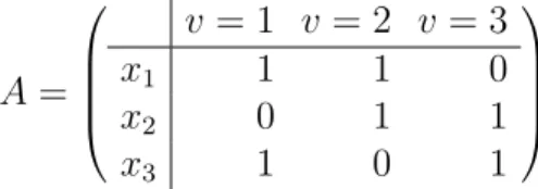
An instance of an alldifferent(x1, . . . , xn) constraint is equivalently represented by an
in-cidence matrix A = (aiv) with aiv = 1 whenever v ∈ Diand aiv= 0 otherwise. For notational
convenience and without loss of generality, we identify domain values with consecutive natu-ral numbers. Because we will want A to be square (with m = |S
xi∈XDi| rows and columns), if there are fewer variables than values we add enough rows, say p, filled with 1s. It is known that counting the number of solutions to the alldifferent constraint is equivalent to com-puting the permanent of that square matrix (dividing the result by p! to account for the extra rows) [Zanarini and Pesant (2010)]:
perm(A) =
m
X
v=1
a1vperm(A1v) (3.1)
where Aij denotes the sub-matrix obtained from A by removing row i and column j.
A = v = 1 v = 2 v = 3 x1 1 1 0 x2 0 1 1 x3 1 0 1
Figure 3.1 Incidence matrix for alldifferent(x1, x2, x3) with D1 = {1, 2}, D2 = {2, 3} and
Since computing the permanent is #P-complete [Valiant (1979)], Zanarini and Pesant pro-posed approximate counting algorithms for the alldifferent constraint based on sam-pling [Zanarini and Pesant (2007)] and upper bounds [Pesant et al. (2012)]. Algorithm 2 reproduces the latter using notation adapted for this article. As each assignment xi = v
in the alldifferent constraint induces a different incidence matrix, a naive approach to compute solution densities is to recompute the permanent upper bound for each assignment. However, our upper bounds are a product of factors F for each variable xi which depend only
on the size of its domain di = |Di| (line 1). Hence if we account for the domain reduction of
the assigned variable (line 5) and of each variable which could have taken that value (line 6) — simulating forward checking — we can compute the solution density of each assignment (line 10) by updating the upper bound UBA calculated for the whole constraint (line 1).
Reusing UBA avoids recomputing upper bounds from scratch. Let cv denote the number of
1s in column v of A. Given that we can precompute the factors, the total computational effort is dominated by line 6 where we do a total of Θ(Pm
v=1c2v) operations: for a given value
v, uv is computed cv times by multiplying cv− 1 terms.
1 UBA = Qx
iF [di] . Constraint upper bound
2 foreach xi ∈ X do
3 total = 0 . Normalization factor
4 foreach v ∈ Di do 5 uxi = F [dF [1]
i] . Variable assignment update
6 uv =Qk6=i : v∈D k
F [dk−1]
F [dk] . Value assignment update
7 UBxi=v = UBA· uxi· uv . Assignment upper bound 8 total += UBxi=v
9 foreach v ∈ Di do
10 SD[i][v] = UBxi=v / total 11 return SD
Algorithm 2: Solution densities for alldifferent, adapted from [Pesant et al. (2012)]
3.1.1 Improved Algorithm
The product at line 6 of Algorithm 2 can be rewritten to depend only on v:
uv = F [dF [di−1]i] Qk : v∈Dk
F [dk−1]
F [dk] . (3.2)
This allows us, as shown in Algorithm 3, to precompute this product for every value (line 1-4) as it does not depend on i anymore, leading to each UBxi=v being computed in constant time
(line 8). We also avoid computing UBA since that factor cancels out during normalization.
Algorithm 3 runs in Θ(Pm
v=1cv) time, which is asymptotically optimal if we need to compute
every solution density (since Pm
v=1cv =Pni=1di). 1 UBv = 1, ∀v ∈ {1, 2, . . . , m} 2 foreach xi ∈ X do 3 foreach v ∈ Di do 4 UBv *= F [dF [di−1] i] 5 foreach xi ∈ X do 6 total = 0 7 foreach v ∈ Di do 8 UBxi=v = F [1] F [di−1]·UBv 9 total += UBxi=v 10 foreach v ∈ Di do 11 SD[i][v] = UBxi=v / total 12 return SD
Algorithm 3: Improved version of Algorithm 2.
3.1.2 Computing Maximum Solution Densities Only
Some search heuristics, such as maxSD, only really need the highest solution density from each constraint in order to make a branching decision. In such a case it may be possi-ble to accelerate the counting algorithm further. We present such an acceleration for the alldifferent constraint.
The factors F in our upper bounds are strictly increasing functions, meaning that for a given value v, the highest solution density will occur for the variable with the smallest domain. Algorithm 4 identifies that peak for each value, knowing that the highest one will be included in this subset. Note however that because we don’t compute a solution density for each value in the domain of a given variable, we cannot normalize them as before (though we at least adjust for the p extra rows). So we may lose some accuracy but what we were computing was already an estimate, not the exact density. The asymptotic complexity of this algorithm remains the same as the previous one, but makes fewer computations: we iterate on each
variable and value once instead of three times. 1 UBv = (F [n−1] F [n] ) p, min v = 1, ∀v ∈ {1, 2, . . . , m} 2 foreach xi ∈ X do 3 foreach v ∈ Di do 4 UBv *= F [dF [di−1] i] 5 if di < dminv then 6 minv = i
7 maxSD = {var = 0, val = 0, dens = 0} 8 foreach v ∈ {1, 2, . . . , m} do
9 SD[minv][v] = F [dF [1]
minv−1]·UBv
10 if SD[minv][v] > maxSD.dens then 11 maxSD = {minv, v, SD[minv][v]}
12 return maxSD
Algorithm 4: Maximum solution density for alldifferent An evaluation of improvements of Algorithm 2, 3 and 4 is given in Section 5.1.1.
3.2 Spanning Tree Constraints
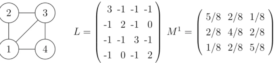
Brockbank, Pesant and Rousseau introduced an algorithm to compute solution densities for the spanningTree constraint in [Brockbank et al. (2013)]. The graph is represented as a Laplacian matrix L (vertex degrees on the diagonal and edges indicated by -1 entries) and Kirchhoff’s Matrix-Tree Theorem [Chaiken and Kleitman (1978)] is used to compute solution densities for every edge (u, v) using the following formula:
σ((u, v), 1, spanningTree(G, T )) = muv0v0 (3.3)
with Mu = (mu
ij) defined as the inverse of the sub-matrix Lu obtained by removing row and
column u from L and v0 equal to v if v < u and to v − 1 otherwise. Given a vertex cover of size γ on a graph over n nodes, computing all solution densities takes O(γn3) time. Figure 3.2 shows an example graph and its Laplacian matrix.
1 2 3 4 L = 3 -1 -1 -1 -1 2 -1 0 -1 -1 3 -1 -1 0 -1 2 M1 = 5/8 2/8 1/8 2/8 4/8 2/8 1/8 2/8 5/8
Figure 3.2 Graph and its Laplacian matrix with γ = 2, meaning we can get every edge density by inverting two submatrices, e.g. L1 (with inverse M1 shown) and L3
With this formula counting-based search heuristics can be used on problems such as de-gree constrained spanning trees (and Hamiltonian paths in particular) with very good re-sults [Brockbank et al. (2013)]. However, they become impractical for large instances because of repeated matrix inversion. The following sections address this problem by proposing two improvements. Note that these improvements remain valid for the recent generalization to weighted spanning trees [Delaite and Pesant (2017)].
3.2.1 Faster Specialized Matrix Inversion
By construction, the sub-matrix Lu we invert has a special form that enables us to use a
specialized algorithm. It is Hermitian (more precisely, integer symmetric). Since the row and column removed from L have the same index u, it is diagonally dominant: |`u
ii| ≥
P
j6=i|`ij|, ∀i.
Its diagonal entries are positive. Therefore it is positive semidefinite or, equivalently, has non-negative eigenvalues. The Matrix-Tree Theorem states that the number of spanning trees is equal to the determinant of Lu, itself equal to the product of its eigenvalues. Therefore each eigenvalue is strictly positive and Lu is positive definite.
A Hermitian positive definite matrix can be inverted via Cholesky factorization instead of the standard LU factorization. Inverting a positive definite matrix requires approximately
1 3n
3 (Cholesky factorization) + 2 3n
3 floating-point operations whereas inverting a general
matrix requires approximately 23n3 (LU factorization) + 43n3 floating-point operations [Choi et al. (1996)]. We therefore expect a two-fold improvement in runtime.
3.2.2 Inverting Smaller Matrices Through Graph Contraction
When branching, if an edge (u, v) is fixed, the Laplacian matrix must be updated to reflect this change. The technique described by Brockbank, Pesant and Rousseau is the following: if it is forbidden, we set luv = 0; if it is required, we must contract it in the graph, meaning
component while keeping a 1 on the diagonal of these vertices to keep the matrix invertible. Figure 3.3 shows an example.
1 2 3 4 L = 3 0 -3 0 0 1 0 0 -3 0 3 0 0 0 0 1
Figure 3.3 Contraction follow-ing assignments e(1, 2) = 1 and e(1, 4) = 1, with 1 as the rep-resentative vertex in connected component {1, 2, 4} 124 3 L = 3 -3 -3 3
Figure 3.4 Connected compo-nent {1, 2, 4} as a single vertex
This way of updating L works but still requires that we invert (n − 1) × (n − 1) matrices to compute solution densities throughout the search. However, as shown in Fig. 3.4, we can view each connected component as a single vertex, leading to smaller Laplacian matrices, and thus smaller matrices to invert as we fix edges.
An evaluation of improvements of Section 3.2.1 and 3.2.2 is given in Section 5.1.2.
3.3 Avoiding Systematic Recomputation
The improvements we presented so far are specific to the alldifferent and spanningTree constraints. In this section we present an additional technique applicable to any constraint in order to avoid recomputation but at the expense of accuracy. Usually at every node of the search tree, before branching, we systematically call the counting algorithm for each con-straint. Suppose we have a spanningTree constraint on a graph with hundreds of vertices and thousands of edges: we may have fixed a single edge with very few changes propagated since the last call to its counting algorithm but the whole computation, involving the expen-sive inversion of large matrices, will be undertaken again even though the resulting solution densities are likely to be very similar. To avoid this we propose a simple dynamic technique: while the variable domains involved remain about the same, we do not recompute solution densities for a constraint but use the latest ones as an estimate instead. For any given node k in the search tree and constraint c, let Sk
c =
P
xi∈cdi. We recompute only if S
k
c ≤ ρScj,
from the root for which we computed solution densities for c. Note that as opposed to a static criterion such as calling the counting algorithm of every constraint at fixed intervals of depth in the search tree, our approach adapts dynamically to individual constraints and to how quickly the domains of the variables in their scope shrink.
CHAPTER 4 PRACTICAL IMPLEMENTATION OF COUNTING-BASED SEARCH IN GECODE
At the start of this Master’s degree, counting-based search heuristics were only available in a private fork of ILOG Solver [IBM (2018)], a commercial constraint programming solver. This made it difficult for other researchers to test our heuristics, hence leading the slower adoption among academia.
Therefore, introducing counting-based search heuristics in a more readily available solver was the first logical step to undertake. For this task, we chose Gecode for the following reasons:
• State-of-the-art performance • Feature-rich
• Good documentation • Free and open-source
Furthermore, from the perspective of a graduate student, modifying Gecode led to a better understanding of constraint programming — both in theory and practice, and made it easier to implement ideas that were central to the other half of this work.
Section 4.1 introduces a basic vocabulary and theoretical setting for understanding Gecode and the following subsections. Section 4.2 explains the required changes to Gecode to support counting-based search. In Section 4.3 we give a quick overview of the counting algorithm we implemented, thus making it possible to design a brancher using counting-based search (Section 4.4).
4.1 Basic Notions in Gecode
This section is not a full introduction to the real inner working of the solver; with close to 2 000 classes and 300 000 lines of C++, Gecode is very complex and such an introduction would not be useful for our purpose.
Instead, we will work under various simplifying assumptions to make it easier to introduce just enough Gecode terminology for understanding the next sections.
All the material in this section will be introduced alongside the same practical problem as in the introduction: solving the partially filled magic square in Fig. 1.1.
4.1.1 Main Loop in Gecode
Under the (naïve) assumption that we must return all solutions, that we always copy the problem state, that we only make binary branching choices (more on that later), and that we explore the search space in a depth-first search fashion, Alg. 5 is a good representation of Gecode’s main loop.
1 Function SOLVE(space)
2 space’ ← PROPAGATE(space) 3 if space’ is invalid then
4 return ∅
5 if space’ is valid then 6 return solution
7 s1, s2 ← BRANCH(space’)
8 return SOLVE(s1) ∪ SOLVE(s2)
Algorithm 5: Solving a constraint programming problem in Gecode, adapted from [Tack (2009)]
According to this algorithm, the first step for solving our magic square is to create a space and pass it to this function. In Gecode, a space is any class inheriting the base class Space and it encapsulates the model and the search component of the problem. Before talking about this function, we will show how we create a space that follows the mathematical model given in Fig. 1.2.
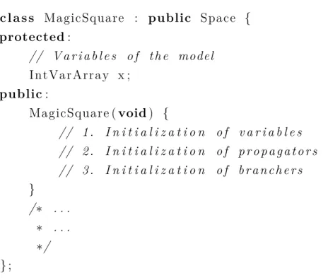
4.1.2 Creation of the Model
Our new class will be called MagicSquare and the model has to be defined inside its con-structor:
c l a s s MagicSquare : public Space { protected : // V a r i a b l e s o f t h e model I n t Va r A r r ay x ; public : MagicSquare ( void ) { // 1 . I n i t i a l i z a t i o n o f v a r i a b l e s // 2 . I n i t i a l i z a t i o n o f p r o p a g a t o r s // 3 . I n i t i a l i z a t i o n o f b r a n c h e r s } /∗ . . . ∗ . . . ∗/ } ;
Figure 4.1 Gecode model for the magic square problem in Fig. 1.2
Variables. First, we provide a set of variables for which we must find an assignment satisfy-ing all the constraints in our problem. We declare 16 variables of domains {1, . . . , 16}, thus already enforcing that all numbers must be between 1 and n ∗ n. By doing so, the first two members of the constraint satisfaction problem P = hX, D, Ci are defined:
// 1 . I n i t i a l i z a t i o n o f v a r i a b l e s const i n t n = 4 ;
x = I n t V ar A r r ay ( ∗ this , n∗n , 1 , n∗n ) ;
Figure 4.2 Variables for model in Fig. 4.1
Propagators. The last member of the CSP model corresponds to the constraints. In Gecode, implementation of constraints are called propagators. These objects are not created directly in the space’s constructor; this responsibility is delegated to post functions that create the right propagators depending on parameters such as the arity or the consistency level of constraints. The constraints of our magic square problem are defined like this:
// 2 . I n i t i a l i z a t i o n o f p r o p a g a t o r s // Matrix−wrapper f o r v a r i a b l e s Matrix<IntVarArray> m( x , n , n ) ; // We c o n s t r a i n v a r i a b l e s a l r e a d y a s s i g n e d r e l ( ∗ this , m( 0 , 0 ) == 1 6 ) ; r e l ( ∗ this , m( 1 , 1 ) == 1 0 ) ; r e l ( ∗ this , m( 2 , 2 ) == 7 ) ; // A l l numbers must b e d i f f e r e n t d i s t i n c t ( ∗ this , x )
// Sum f o r e a c h row / column / d i a g o n a l const i n t S = n ∗ ( n^2+1)/2
// Rows and columns must b e e q u a l t o S f o r ( i n t i = 0 ; i < n ; i ++) { l i n e a r ( ∗ this , m. row ( i ) == S ) ; l i n e a r ( ∗ this , m. c o l ( i ) == S ) ; } // D i a g o n a l s must a l s o b e e q u a l t o 34 l i n e a r ( ∗ this , m( 0 , 0 ) +m( 1 , 1 ) +m( 2 , 2 ) +m( 3 , 3 ) == S ) ; l i n e a r ( ∗ this , m( 0 , 3 ) +m( 1 , 2 ) +m( 2 , 1 ) +m( 3 , 0 ) == S ) ;
Figure 4.3 Constraints for model in Fig. 4.1
4.1.3 Creation of the Search Strategy
The second component — the search strategy — is also defined inside the space constructor and created by post functions.
Branchers. The search strategy is represented by branchers. A brancher is responsible for giving a branching choice when the propagators are no longer able to do constraint propagation. The following function will create a brancher that will select the variable with
the smallest domain and branch on the smallest value. // 3 . I n i t i a l i z a t i o n o f b r a n c h e r s
branch ( ∗ this , x , INT_VAR_SIZE_MIN ( ) , INT_VAL_MIN ( ) ) ; Figure 4.4 Brancher for model in Fig. 4.1
4.1.4 Solving the Problem
The previous components in the constructor are enough for describing our magic square. Aside from some small details, we now have a Space subclass for our problem named MagicSquare. Finding a solution is done by creating a MagicSquare object and passing it to a search engine such as depth-first search. As stated in Section 4.1.1, this corresponds to passing our object to the function SOLVE of Alg. 5. When doing so, the following will happen at each line:
2 Constraint propagation is done on the MagicSquare space; all instantiated propagators are going to filter variable domains according to their consistency levels until no more pruning can be done. At this point, the space will be at a fixpoint and will correspond to Fig. 1.5.
3-6 If any constraint is violated or any variable domain becomes empty while doing con-straint propagation, the space will be invalid causing the function to return ∅ as no solution is possible. Otherwise, if all variables are fixed, we return the solution. Neither is the case in our example, so we go to line 7.
7 Here, we must make an hypothesis. Our brancher will give the branching choice x5 = 2.
8 We split the space in two parts, like in Fig. 1.4. We will first call SOLVE(s1) and redo
the whole process given we have a new space modified by the branching choice.
Eventually, Gecode will find a solution using our model after 8 failures.
4.2 Basic Structure for Supporting Counting-Based Search in Gecode
The magic square can now be solved using the previous model. Our next step is to replace the brancher posted in Fig. 4.4 with a custom brancher using counting-based search.
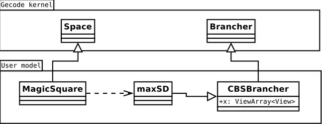
Gecode is modular and extensible. A user is not limited to constructing a space that uses only available branchers and constraints in Gecode; it is possible to create custom branchers and propagators by inheriting from the base classes Brancher and Propagator respectively. However, the abstractions provided were not sufficient to implement a brancher using counting-based search heuristics and this section describes the changes required to Gecode for this task. This was accomplished with one primary goal: make as few modifications to Gecode as pos-sible. As we can see in Fig. 4.5, MagicSquare and our brancher can be created in the user model (a program that uses Gecode as a library). Our goal is to replace the function in Fig. 4.4 with a function posting a brancher of our own that uses counting-based search and Alg. 1 to make branching decisions.
Before doing so, we need a method for triggering solution density computation in propagators for generating hpropagator, variable, value, densityi tuples (i.e. a virtual method that we can overload to specify counting algorithms for different propagators).
Afterwards, even if we are able to call this method in a brancher and retrieve all tuples, we still won’t be able make a CBS branching heuristic; making those heuristics require aggregating solution densities on propagators, variables and values. In Gecode, this is impossible as there’s no unique id for variables and accessing them from different propagators can lead to different views of the same domain — an injective function may or may not be applied before access.
Addressing those concerns requires modifying multiple classes in the Gecode kernel and Int module, resulting in a small patch that can be divided in three parts, each of them described in the following subsections. After these modifications, we will be able to make our counting-based search branching heuristic.
Figure 4.5 Modeling the magic square with a custom brancher using Gecode
Our goal — making as few modifications to Gecode as possible — may seem odd at first sight. The design we are presenting is actually our second iteration. In our first design, we did not pay attention to this factor and ended up with a patch of approximately 1500 lines. While it worked, its complexity made it very difficult to collaborate with the developers of Gecode. This is why we did a complete redesign, keeping only what is essential, to facilitate the integration of our patch.
4.2.1 Unique IDs for Variables
As implied in Alg. 1, we need a unique id for each constraint and variable in the model to compute a branching decision. Gecode did provide an id for propagators, but not for variables.
In Gecode, there are two possible abstractions over variable implementations (the object encoding the actual domains of variables): variables and views.
Variables are simply a read-only interface for variable implementations and they are used for modeling (see the protected member in Fig. 4.1). This makes sense because the model is declarative; we don’t interact directly with domains.
On the other hand, views act as interfaces to variable implementations for propagators and branchers. They offer the ability to prune values from variable domains, and for this reason, must not be used for modeling.
For doing density aggregation, we need a unique id for variable implementation that is ac-cessible from views. When creating a new variable implementation, its constructor has a
reference to the current space. Therefore, a global counter in Space that we increment in the constructor of VarImp can be used as a unique id. Accessing this new member amounts to adding a new method id() to the following classes:
• VarImp. Base-class for variable implementations.
• VarImpView. Base-class for variable implementation views. Gives a direct access to the domain.
• DerivedView. Base-class for derived views, for which an injective function may be applied before accessing the domain.
• ConstView. Base-class for constant views — views that mimic an assigned variable.
Those changes correspond to commit d4aa3 in https://github.com/Gecode/gecode.
4.2.2 Methods for Mapping Domains to their Original Values
Like previously said, propagators access variables via views. A view can remap every value of its domain. For example, accessing a variable with domain D = {1, 4, 8} from a MinusView will yield D0 = {−1, −4, −8}. Two propagators may use different views to the same variable, meaning we can’t group densities by domain values.
To fix this, we added the following method to all views:
// / Return r e v e r s e t r a n s f o r m a t i o n o f v a l u e a c c o r d i n g t o v i e w i n t b a s e v a l ( i n t v a l ) const ;
Given that propagators already have unique ids, it is now possible to do aggregation of densities in CBS_HEUR() and Alg. 1 becomes:
1 SD = {}
2 foreach constraint c(x1, . . . , xn) do
3 foreach unbound variable xi ∈ {x1, . . . , xn} do 4 foreach value d ∈ Di do
5 SD[id(c)][id(xi)][xi.baseval(d)] = σ(xi, d, c)
6 return CBS_HEUR(SD) . Return a branching decision using SD
Algorithm 6: Modified version of Alg. 1 that uses unique ids for propagators and vari-ables and take into account view transformations.
4.2.3 Computing Solution Distributions for Propagators
In Gecode, we can iterate over active propagators of the current space inside a brancher, but we do not have access to the internal state of propagators and their variables. To compute solution densities in propagators, a method must be added to the base class Propagator: typedef s t d : : f u n c t i o n <void ( unsigned i n t prop_id ,
unsigned i n t var_id ,
i n t v a l , double d e n s )> S e n d M a r g i n a l ; v i r t u a l void s o l n d i s t r i b ( Space& home , S e n d M a r g i n a l s e n d ) const ;
SendMarginal is a function that inserts solution densities in SD. Given we create a custom brancher with a method named sendmarginal and a private member named SD, making choices in our brancher will look like the following algorithm:
1 SD = {}
2 foreach constraint c do
3 c.solndistrib(space, sendmarginal)
4 return CBS_HEUR(SD) . Return a branching decision using SD
Algorithm 7: Modified version of Alg. 6 closer to how Gecode interacts with propagators.
Those changes correspond to commit 6957b in https://github.com/Gecode/gecode. With these three commits, it is possible to create a counting-based search brancher given we im-plement specialized counting algorithms for constraints by overloading solndistrib in the correct propagators.
4.2.4 Accessing Variable Cardinalities Sum in Propagators
Lastly, a final method is required in Propagator if we want to make counting-based search efficient.
If all variable domains in a propagator stay identical after branching and propagating, we can reuse previous calculated densities when making the next branching choice. However, as shown in Alg. 7, we recompute every solution distributions from scratch each time we make a choice. We can fix this by adding the following method in Propagator:
typedef s t d : : f u n c t i o n <bool ( unsigned i n t var_id )> I n D e c i s i o n ; v i r t u a l void domainsizesum ( I n D e c i s i o n i n , unsigned i n t& s i z e ,
As we can only remove values from domains during propagation, a variable with equal cardi-nality before and after propagation has the same domain. This logic holds true for an entire propagator: if the sum of its variable domain cardinalities is equal before and after propaga-tion, all the variables in the propagator are unchanged, meaning we don’t have to recompute densities. Those changes also correspond to commit 6957b in https://github.com/Gecode/ gecode.
This method will be used in our brancher to avoid unnecessary recomputation of solution densities.
4.3 Counting Algorithms
Section 4.2 gave the basic structure for creating a custom brancher that uses counting-based search. However, we still need counting algorithms for propagators created when specifying a model to get solution densities and make branching choices.
Let’s take the example of our Magic Square Problem again. When instantiating the model of Fig. 4.1, the following propagators are created (using their default consistency):
• A single Int::Distinct::Val propagator for the distinct constraint. • Several Int::Linear::Bnd propagators for the linear constraints.
Thus, we need to overload Int::Distinct::Val::solndistrib and Int::Linear::Bnd:: solndistrib to specify counting algorithms (alongside domainsizesum for both classes). Without this, our brancher will not be able to give branching choices; the more propagators we support, the more problems we can solve.
In this thesis, we implemented counting algorithms for distinct, linear, and extensional (regular expression) constraints [Pesant and Quimper (2008)][Zanarini and Pesant (2010)]. Annex A gives implementation details about each counting algorithm alongside a generic template for implementing them.
4.4 Creating a Brancher Using Counting-Based Search
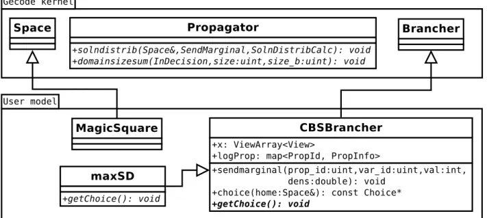
Figure 4.6 Principal components in relation with CBSBrancher
The logic for making branching choices — described in Alg. 7 — is located in the method choice. This method stores solution densities in a map called logProp and uses domainsize-sum to evaluate if densities for a given propagator need to be recalculated between propaga-tions.
As counting-based search is a family of branching heuristics, the concrete brancher is cre-ated by inheriting from CBSBrancher and overloading getChoice for specifying how we make choices from all hpropagator, variable, value, densityi tuples. In this case, we use the branch-ing heuristic maxSD, but other heuristics are possible such as aAvgSD, maxRelSD, etc. (as explained in [Zanarini and Pesant (2007)]).
In Section 5.2, we benchmark maxSD against other generic branching heuristics for three different problems.
CHAPTER 5 EMPIRICAL EVALUATION
In this chapter, an empirical evaluation of all work discussed in Chapter 3 and Chapter 4 is given. Section 5.1 evaluates the improvements to the alldifferent and spanningTree constraints. Section 5.1.3 evaluates the generic method proposed in Section 3.3 to avoid calling counting algorithms at all nodes. Finally, Section 5.2 compares our implementation of CBS with other generic branching heuristics in Gecode.
All graphs in this chapter are interpreted the same way across all benchmarks, with each benchmark accompanied by two graphs. The first one gives the percentage of instances solved with respect to the number of failures — if we have 100 instances of a particular problem and a cutoff of 1000 failures when backtracking, f (1000) = 40 means that we are able to solve 40 instances. The second graph is similar except time is used as the cutoff.
5.1 Impact of our Contributions
5.1.1 Acceleration of alldifferent
The Quasigroup Completion Problem consists in filling a m × m grid with numbers such that each row and column contains every number from 1 to m (#67 in CSPLib [Pesant (2018)]). It is very similar to Sudokus with the only difference being that the grid is not separated in sub-grids where all numbers must be different. Surprisingly, this makes the problem a lot harder.
This problem can be described using an alldifferent constraint on each row and column, making it ideal for testing our improvements to its counting algorithms. Gecode’s distribution already includes a model with branching heuristics afc (weighted degree) and size (smallest domain), both with lexicographic value selection. The focus of this experiment is to compare the performance of maxSD using Algorithm 2, 3 and 4, but we also tried the other generic heuristics for comparison.
We use 20 instances of sizes 90 to 110 with 25% of entries filled, generated as in [Gomes and Shmoys (2002)]. That ratio of filled entries may not yield the hardest instances for that size but our goal here is to have a lot of shared values between variables in order to emphasize the improvement of Algorithm 3 over 2.