UNIVERSITÉ DE MONTRÉAL
CONTRIBUTION TO THE STUDY OF THE DIRECT AND INVERSE
PROBLEM IN ELECTROMYOGRAPHY (EMG)
POOYA MAGHOUL
DÉPARTEMENT DE GÉNIE ÉLECTRIQUE ÉCOLE POLYTECHNIQUE DE MONTRÉAL
MÉMOIRE PRÉSENTÉ EN VUE DE L’OBTENTION DU DIPLÔME DE MAÎTRISE ÈS SCIENCES APPLIQUÉES
(GÉNIE ÉLECTRIQUE) DÉCEMBRE 2012
ÉCOLE POLYTECHNIQUE DE MONTRÉAL
Ce mémoire intitulé:
CONTRIBUTION TO THE STUDY OF THE DIRECT AND INVERSE
PROBLEM IN ELECTROMYOGRAPHY (EMG)
présenté par: MAGHOUL Pooya
en vue de l’obtention du diplôme de Maîtrise ès sciences appliquées a été dûment accepté par le jury d’examen constitué de :
M. BRAULT Jean-Jules, Ph.D., président
M. CORINTHIOS Michael J., Ph.D., membre et directeur de recherche M. MATHIEU Pierre A., Ph.D., membre et codirecteur de recherche M. VINET Alain, Ph.D., membre
DEDICATION
This thesis is dedicated to both my parents. My father, Behzad maghoul, did not only raise and nurture me but also taxed himself dearly over the years for my education and intellectual development.
My mother, Sima khoshnevis-asl, has been a source of motivation and strength during moments of despair and discouragement. Her motherly care and support have been shown in incredible ways.
ACKNOWLEDGEMENTS
I would like to express my sincere gratitude to Prof. Bertrand for his support of my M.Sc. study and research, for his patience, motivation, enthusiasm, and immense knowledge.
Besides him, I would like to thank the rest of my thesis committee: Prof. Vinet, Prof. Brault, for their times which they spent to me.
Last but not the least, I would like to thank my family: my parents (Sima Khoshnevis-asl and Behzad maghoul) and my sister (Pooneh Maghoul), for giving supporting me spiritually throughout my life.
RÉSUMÉ
On dispose maintenant de prothèses myoélectriques du membre supérieur pouvant produire plusieurs mouvements utilisés dans les activités de la vie quotidienne. Pour les activer, la présence de 6 compartiments anatomiques dans le biceps brachial pourrait être exploitée. Pour aider à vérifier si ces compartiments ont pu être activés lors de contractions accomplies par des sujets normaux, l'utilisation d'un modèle direct et inverse pourrait être très utile. Pour initier le développement de ces modèles, des données provenant d'expériences où, un contenant cylindrique, encerclé de 16 électrodes et rempli d'une solution saline a été utilisé. Dsns ce bassin, jusqu'à 3 dipôles avaient été introduits à des positions connues. Pour poursuivre la validation du modèle inverse, on a simulé des signaux associés à 3 regroupements de 5000 fibres musculaires placées à des positions connues à l'intérieur d'un bassin cylindrique virtuel. Finalement, les signaux EMG recueillis au-dessus du biceps de sujets normaux lors d'expériences visant à activer individuellement ou en groupe les 6 compartiments du biceps ont été analysés. On a identifié 3 zones d'activité: une dans le chef court et 2 dans le chef long du muscle. Dans le chef court, l'intensité du dipôle a été similaire dans les 6 conditions testées tandis que sa position était variable. Dans le chef long, la position des deux zones actives est moins variable mais leur intensité très variable. Alors que les 3 zones d'activité peuvent être considérées comme étant situées dans divers compartiments du biceps, on a trouvé que leur position lorsque reportée sur une illustration générique d'une coupe transversale de l'avant-bras, l'une des zones était localisée au niveau de la couche de graisse et celle de la peau. Il semble donc possible d'identifier dans le biceps des zones d'activité associables à ses compartiments. Toutefois étant donné que certaines de ces zones pourraient se situer en dehors du muscle, la présence des couches de gras et de la peau doivent être introduites pour un modèle plus réaliste du bras lors d’études portant sur le problème direct et inverse en EMG.
Mots-clés: Biceps brachial, compartiments, matrice d'électrodes, EMG, modèle direct et inverse, contrôle de prothèses myoélectriques.
ABSTRACT
In the context of improving the control of upper arm myoelectric prostheses capable of producing various useful movements for daily life activities, the presence of up to 6 anatomical compartments within the biceps brachii can be exploited to increase the number of potential control sites. To help identify where activity could occurs within the biceps during different contractions accomplished by normal subjects, a direct and an inverse model could be very useful. To develop such models, we started with the reproduction of previously collected data obtained with 16 equally spaced electrodes circling a tank filled with a saline solution. Up to 3 dipoles were placed at known positions within the tank. To further test the inverse model, simulated data obtained from the activity of 3 groups of 5000 closely packed single fibers placed at known positions within a virtual tank similar to the real one were analyzed. Finally, EMG signals collected over the biceps brachii during experiments aimed at activating individually or in groups the 6 compartments of the biceps where analyzed in 6 conditions. Three zones of activity were found: one in the short head of the muscle and 2 in its long head. In the short head, the dipole intensity was similar in the 6 conditions tested while its position was variable. In the long head, the position of the two active zones was less variable but their intensity was quite variable. While those 3 zones of activity could be considered to be located in 3 of the 6 muscle’s compartments, when their position was overlaid on a generic cross-section image of the upper arm, one of the zones was outside the muscle tissue. It thus appears possible within the biceps, to identify active zones associable to the muscle’s compartments. However, considering that some of the detected positions could be over the fat and skin layers, those layers should be introduced for a more realistic upper arm model when studying the EMG direct and inverse problem.
Keywords: Biceps brachii, compartments, electrode array, surface EMG, direct and inverse
TABLE OF CONTENTS
Dedication ... iii
Acknowledgements ... iv
Résumé ... v
Abstract ... vi
Table of contents ... vii
List of tables ... ix
List of figures ... x
List of abbreviation ... xvi
Chapter 1 Introduction ... 1
Chapter 2 Litterature Review ... 6
2.1 Muscles ... 6
2.2 EMG recording techniques ... 14
2.3 Direct Problem ... 16
2.4 Inverse Problem………. ... 33
2.4.1 Over-determined method ... 34
2.4.2 Under-determined method ... 38
2.4.3 Single Source Localization ... 39
2.4.4 Discriminating brachialis, BB and triceps ... 40
2.4.5 Results in three dimensions ... 43
Chapter 3 Methodology ... 46
3.1 Direct Model ... 46
3.2 Inverse Model ... 54
3.2.1 Genetic Algorithm (GA)... 54
3.2.2 Nonlinear Conjugated Gradient (NCG)... 58
Chapter 4 Results ... 60
4.1 Tank data ... 60
4.2 Simulated EMG signal ... 68
4.3.1 Result with subject PM ... 79
4.3.2 Result with subject MM ... 82
Chapter 5 Discussion and conclusion ... 84
APPENDIX 1– Using Matlab optimization toolbox with GAI programs ... …94
APPENDIX 2– Results for simulated signals (3 dipoles) ... .97
APPENDIX 3- Single fiber extracellular action potentials..……….98
APPENDIX 4– Cylinder model with three concentric layers ... 109
APPENDIX 5– Illustration of the processing steps for a simple situation ... 112
LIST OF TABLES
Table 2.1 Comparison between the finite difference method (FDM), the discretized integral method called boundary element method (BEM) and the analytic ... 17 Table 2.2 Factors that influence the surface EMG ... 23 Table 2.3 Tissue Composition of Models I–V ... 29 Table 2.4 Conductivity () and relative permittivity () of muscle, fat and skin tissue as ob-
tained in the litterature making 4 realistic models to be compared to the idealized one ... 32 Table 2.5 Normalized activations and their reconstructions in the two different conditions when
biceps and brachialis were activate alone in each simulation ... 44 Table 3.1 Initial 20 chromosomes: associated to a dipole characteristics ... 56 Table 3.2 Sample of 10 parents and their offsprings ... 57 Table 4.1 Effect of the addition of 3 different white gaussioan noise levels on the characteristics
when the mobile dipole was moved from 10 to 70 mm toward the center of the tank. Values in red indicate negative differences i.e. smaller than expected results ... 66 Table 4.2. Peak frequency for each condition test in different subjects………78
LIST OF FIGURES
Fig 1.1 Generic representation of a cross-section of the arm with the skin, the fat (yellow), muscles (red) and the humerus bone (at the center) of the upper arm. The biceps is at the top of the illistration with hypothetical divisions representing its 6 compartments……….4 Fig 2.1 A. Bones of the arm attached to the shoulder articulation. B. Transverse view of the arm.
C. Structure and components of a squelettal muscle D: Illustration of the shortening of 3 sarcomeres ... 7 Fig 2.2 A. Schematic of a neuron with the different concentrations of Na+ and K+. B. Curve of
action potentoial ... 8 Fig 2.3 Axons of 2 motoneurons extending from the spinal cord to a muscle ... 8 Fig 2.4 Anatomic structures of the transverse tubules and of the sarcoplasmic reticulum system in a single skeletal-muscle fiber ... 10 Fig 2.5 A. Heavy chains of myosin molecules form the core of a thick filament. B. The two
globular heads of each myosin molecule extend from the sides of the filament forming a cross bridge. C. A molecule of troponin is bounded to a molecule of tropomyosin and that association prevents interaction with the myosin cross bridges. D. Four stages of a cross-bridge cycle ... 11 Fig 2.6 A. The load pulling on the muscle is constant and an isotonic contraction is produced
when the muscle is stimulated. B. The length of muscle is kept constant and an isometric contraction is produced... 11 Fig 2.7 A. The response of three types of motor units when electrically stimulated and their
resistance to fatigue upon continuous stimulation. B: The size or Henneman principle .. 12 Fig 2.8 Posterior view of the biceps brachii where asterisks indicate neuromuscular
compartments in the long and short head ... 13 Fig 2.9 Schematic representation of motoneurons and compartments of one muscle ... 14 Fig 2.10. Illustration of a concentric needle electrode inserted close to the muscular fibers... 15 Fig 2.11. A. Surface electrodes and surface EMG signal over the BB. B. Linear array
combination of surface electrodes. C. an electrode array of 3 x 8 electrodes used to collect signals around the arm as used in Liste des sigles et abréviations ... 16 Fig 2.12. Different recording of EMG signals A. Monopolar B. Single differential (SD) C.
Double differential (DD) ... 16 Fig 2.13. Two concentric cylinders of finite dimensions to model singlr fiber extracellular action
Fig 2.14. A.Three concentric cylinders simulating muscle tissue, fat and skin layer.B.Simulated signals when the active fiber is placed at various depths (FD) in a homogeneous volume conductor. C: Simulation results for a motor unit composed of 300 fibers at a depth of 5
mm under the skin ... 19 Fig 2.15.Spatial and spatial frequency domain potential distributions at the skin surface and
directly over the muscle as generated by a fiber located at 2 mm under the skin ... 20 Fig 2.16. A. Structure of a spatial electrode matrix. B: Block diagram of anisotropic tissue and
isotropic tissue (fat and skin) ... 20 Fig. 2.17. a. Volume conductor models with bone-muscle, bone-muscle-fat, and bone-muscle-fat- skin. b. Lateral view of the volume conductor with simulated finite-length muscle fibre. c. Configurations of 3 filters with their associated weights for each electrode ... 21 Fig 2.18. Transverse selectivity (TS) between peak-to-peak amplitude of signals ... 22 Fig 2.19 A: Simulation of single MUAP measured with a pair of electrodes placed between the
innervation zone and a tendon. B: Changes in MU potential waveform (normalized
maximum values) due to the influence of fiber depth, fat thickness and fiber length. C and .D: Power spectral densities of the MUAPs in different conditions... 24 Fig.2.20 Insertion of a circular inhomogeneity in an otherwise homogeneous volume conductor
perturbs the surface potential. a) Perturbation (small amplitude wiggles) on the impulse response b) Signal associated of the impulse current source c) Contours of the
perturbation effect for 3 positions of the current source ... 25 Fig 2.21 a) volume conductor perpendicular to the active fiber with an inhomogeneous sphere
placed. b) Four spatial filters were considered: monopolar recording, longitudinal single differential (LSD), double differential (LDD) and normal double differential (NDD). c) Signals obtained with the 4 spatial filters under 3 volume conductor conditions ... 26 Fig. 2.22 A: Surface electrode potential over the phantom as obtained with a FEM model B:
Transverse view of the potential distribution ... 28 Fig. 2.23 Cross section of the 4 components model (bone, muscle, fat, skin) with the 5 positions
considered for the bone ... 28 Fig. 2.24 A. Action potential detected the surface of fiber in 4 of the models of Table 2. B. For
each of the 4 models, RMS value of surface potentials above the active fiber as its depth increased. C. amplitude of spectrum median frequency of surface potential when fiber depth increased ... 29 Fig 2.25 A: Comparison of the RMS value and median frequency in model I and model IV B:
Rate of decay of surface potential RMS value ... 30 Fig 2.26 A. Magnetic resonance image of a transverse section of an human upper arm. B. Image
model of MRI. C: idealized cylindrical model of the image at the left ... 30 Fig. 2.27 An anatomical based volume conductor and location of excitation and recording surface electrodes ... 31
Fig. 2.28 Simulated surface AP for a fiber is located below the skin surface. Left and right
columns of results are for 2 different material properties ... 33 Fig. 2.29 Surface plots of a measured MUAP (upper left) and its contour plot (lower left) ... 36 Fig. 2.30 Potentials detected by 16 surface electrodes placed around the upper arm during a weak contraction ... 36 Fig 2.31 A: Experimental surface EMG signal collected over the BB. B: Power spectrum
of the signal. C: FEM of the upper arm and location of one current source ... 37 Fig 2.32 A. Upper arm MRI. B: 3D COMSOL model of the upper arm. C: FEM mesh of a slice
of the arm made of tetrahedral elements ... 38 Fig 2.33 Single tripole source localization under various inverse model variables ... 39 Fig 2.34 Reconstruction of the current sources for 5 conditions. A: Results obtained with 215
signal points potentials B: Results with the second derivative of the 215 data points. C: Current of sources reconstructed with only 56 points ... 40 Fig. 2.35 Relative power contribution of the upper arm muscles to total power (100%) a: during
flexion with main activity in the biceps and brachialis. b: during extension with activity in the 3 muscles. a-s: synthetic data used for simulating a flexion and result are very close to the real ones in a. b-s: synthetic data for extension where activity in the triceps is large but a significant amount of activity in the brachialis and biceps is also present. Less activity in the biceps and brachialis is obtained when only monopolar signals are used either with a ring of 56 sites (b-m1) or with 215 sensors (b-m2) ... 41 Fig 2.36 A. Upside down MRI of upper arm muscles. B. Modeling upper arm muscles in 4 areas:
1 and 4: Triceps; 2: Brachialis 3: Biceps ... 41 Fig. 2.37 Reconstruction results with different regularization functions when sources are only in
region 1 ... 42 Fig. 2.38 Results with different regularization functions when sources are only in region 4 ... 43 Fig. 2.39 (a). MRI of upper arm. (b) 3D geometry constructed with COMSOL ... 43 Fig. 2.40 Visualization of 3D reconstructed activity with and without D. (a and b):when only the Biceps is active, (c and d): when only the Brachialis is active ... 44 Fig 3.1 A: Photo of the tank circled with 16 equidistant Ag/AgCl electrodes with a dipole near
the border. B: top view schematic of the tank. C: Representation of a dipole made of two small sintered Ag/AgCl cylinders ... 46 Fig 3.2 A: position of an electrode (point O) at the periphery of the tank B: coordinates of the
dipole. C: top view of the tank with the electrodes and a dipole position. D: Side view of the dipole location relative to the recording electrodes ... 47
Fig 3.3 The image phenomenon from the front section where the dipole is positioned at
𝑧′(𝜌′𝜑′𝑧′) ... 48
Fig 3.4 Model representing a portion of a fiber membrane shown as a repetitive network of finite length ... 50
Fig 3.5 Illustration a charge distribution on the axis of the fiber. B: extracellular SFAP ... 52
Fig 3.6 The frequency response of electrode ... 53
Fig 3.7 Flowchart of a GA and nonlinear optimization ... 55
Fig 3.8 Flowchart of the nonlinear conjugate gradient (NCG) optimization process ... 59
Fig 4.1 A. Top view of the tank with one dipole placed in front and at 5 mm from electrode #5 before being moved radially toward the tank center. B. Inverse model results as the dipole was moved toward the center ... 60
Fig 4.2 A. RMS values collected under each electrode when the dipole was at 80 mm from the tank’s border. Maximum value is under electrode #6 while is should have been under electrode #5. B. due to the angular misalignment, the dipole distance from the center is greater than expected ... 61
Fig 4.3 Simulation results obtained with the direct and inverse models when a single dipole is moved toward the tank’s center (N.S= non significant ... 61
Fig 4.4 Inverse model results when a dipole is moved toward the center while another one is fixed at 10 mm from the border from Filion directory multiple_sensibilite_radiale) ... 62
Fig 4.5 Results of the inverse problem when a dipole is moved angularly with the second one is kept in front of electrode #5 ... 63
Fig 4.6 Results of the inverse problem when 2 dipoles are at a fixed position and the third one moved radially in steps of 5 mm toward the center of the tank. Same current intensity feeding each dipole ... 63
Fig 4.7 From the same dataset of the previous figure, comparison between experimental RMS values and inverse model results for the 10 and 25 mm position of the mobile dipole .... 64
Fig 4.8 Results of the inverse problem when a dipole has angular movement and two others remained fixed close to electrode #9 and #10 ... 65
Fig 4.9 Results of the inverse model when 3 dipoles are in fixed position but their relative intensity is for position 1: 1:1:1. for 2: ½:1:1. for 3: ½:½:1, for 4: ½:½:½, for 5: ¼:1:½, for 6: 1:1:½, for 7: 1:½:½ and for 8:1:½:1 (from Filion 3_dipoles_exp_D directory) .. 65
Fig 4.10 Sinusoidal signal (45 Hz) to which different S/N white noise ratio was added. A: 30 dB; B: 20 dB; C: 10 Db ... 66
Fig 4.11 The amplitude of frequency analysis A. Dipole 70 mm from the border B. dipole 10 mm from the border ... 67 Fig. 4.12 A: Diagram where s represents a charge distribution on the axis of a fiber (r=0). The
perpendicular distance from the fiber axis, a represents the fiber radius .The distance between the charge distribution(s) and the recording point P is (z-s). B: extracellular SFAP obtained with r slightly larger than a which is 20 µm. C. Simulation of SEMG obtained with the summation of 1000 SFAPs of random amplitudes as observed at a z-s and r value of respectively aa and bb mm. D: a sum of 2500 SFAPs and of 5000 SFAPs in E under the same measuring point ... 70 Fig 4.13 Dipole positions considered in the simulation. Size of the circles is proportional to the
intensity associated to each dipole ... 71 Fig. 4.14 Linear core-conductor model representing a portion of the fiber membrane. For
graphical representation the structure is shown as a repetitive network of finite length z, but in fact z 0; the analysis is based on the continuum. The open box is a symbol representing the equivalent circuit of the membrane, which depends on the membrane state, namely a passive structure during the resting period and a circuit with
time-dependent components during the active phase ... 71 Fig 4.15 Blue lines: results obtained with sinusoidal current applied to 3 dipoles in the tank as in
Fig.4.13 and red lines results are associated to 3 dipoles each made up of 5000 SFAPs. Mean absolute value (MAV) potential is used in both situations and the 3 dipoles are at 10 mm from the tank border Relative intensity of the dipole in front of eletrode #3 was 2, it was 1 for the dipole in front of electrode #7 , an 4 for the dipole in front of #11 as easily seen in panel A..Results in panel B were obtained when each dipole position was
angularly moved anticlockwise by 11.25° (half angular position between 2 adjacent electrodes). Between electrode #10 and #12 the results were identical and the blue line is hidden below the red one. Results in panel C were obtained when the dipoles are in front of electrode #3, #4 and #5 ... 72 Fig 4.16 The FFT of signals at electrodes 2 to 9 around the tank when three dipoles are in the
tank which has one isotropic environment ... 73 Fig 4.17 The smooth FFT of electrodes 1 to 5 ... 74 Fig 4.18 A) The fitness value in GA B) The values of radius, angles and intensities C) Error in
NO method.The first third values are radial distance from the center, the second third values are the angle values and third third values are the relative intensities and the last one is the phase of signal ... 75 Fig 4.19 Comparison between the forward and inverse model results. with 3dipoles ... 75 Fig 4.20 A. Three body positions used to collect the data. B. Three hand positions experimented
during each body position. C. Five pairs of surface gold–plated electrodes where placed over the short (S) and long (L) heads of the BB muscle . D.Electrode matrix used ... 76
Fig 4.21 Ten EMG signals collected over the BB during a 20% MVC contraction while the subject was seated and the hand in right elbow flexed ~100°. Same amplitude scale for each signal ... 76 Fig 4.22 FFT of the 10 signals displayed in the previous figure ... 77 Fig 4.23 A. Smoothed version of the FFT shown in the previous figure. B. Ten Welch spectra of
Fig.4.17 signals with their mean value (dashed line) with a peak at 49 Hz ... 78 Fig 4.24 RMS values for supination condition when the subjects asked to sit and stand with 1 kg
load in wrist that shows in sitting condition one area activites is around electrode 2, another around electrode 5 and third around electrode 8. In standing condition, the activity area is one around electrode 3, second is around electrode 6 and the third around electrode 8………..79 Fig 4.25 Three experimental trials of seated subject PM when his hand was supinated (Sup) and
pronated (Pron). The figures around the tip of each spoke is the MAV value (µV) of the signal collected by each electrode Both in supination (Sup) and pronation (Pron), 2 dipoles are associated to the activity within the short head and one in the long head of the BB. In the figure, 0° is considered to be at the left of the circle and angular values (phi) are measure clockwise. The position of an active area (rho) is from the border of the circle used to represent the arm and I is a relative intensity of each dipole. For this subject, the radius of the circle was 43 mm ... 80 Fig 4.26 Same situations as in the previous figure except that subject PM was standing up with
his arm extended laterally without load. Positions of the dipoles are somewhat similar to the previous figure except that the intensity of the red dipole is now smaller than for the 2 others and that the blue and black dipole relative angular position is different depending on the hand position... 81 Fig 4.27 Three experimental trials of the standing up subject PM with a 1 kg load at the wrist.
While the detected activity is similar to the standing position without load, the intensity of the blue dipole is now the largest.while the red dipole position appear to be shifted
clockwise particularly when the hand was pronated ... 82 Fig 4.28 Averaged results obtained for the 3 trials of the MM subject as collected in 3 body
positions. Each lenght of a spoke is proportionnal to the average MAV values obtained from the 3 individual trials ... 83 Fig 5.1 In the left and middle column, superposition of the inverse model results with a schematic
representation of the hypothetical repartition of the 6 compartments within the biceps whose lower border is represented by the horizontal red line. Each figure within the circles is related to the intensity of a zone of activity. In the right column, results obtained in pronation are superposed to a generic cross-section illustration of the anatomical upper arm structures at the level of the recording electrodes. White color has replaced the red one used in the center column for one of the zone of activity. Color is only used for visualization purposes, it does not tag a particular zone of activity ... 87
List of abreviations
Ach Acetylcholine
AP Action potential
BB Biceps Brachii
BEM Boundary Element Method
BR Brachialis
CMRR Common Mode Rejection Ratio
DD Double Differential
ECG Electrocardiography
EEG Electroencephalography
EMG Electromyography
FDM Finite Difference Method
FEM Finite Element Model (FEM)
FF Fast-Fatigable
FFR Fast Fatigue-Resistant
IAP Intracellular action potential LAURA Local Autoregressive Average LDD Longitudinal double differential LSD Longitudinal single differential
MEG Magnetoencephalography
MN Motoneuron
MU Motor unit
MUAP Motor Unit Action Potential NDD Normal Double Differential
SD Single Differential (SD)
SFAP Single Fiber Action Potential
TR Triceps
CHAPTER 1: INTRODUCTION
The direct and inverse problem is a mathematical approach used in many branches of science and mathematics such as computer vision, medical imaging, machine learning and many other fields including electrophysiology. In the forward or direct problem, a known source is placed within a known volume conductor but the signals across the medium are not known and needed to be calculated. A single solution is obtained with an accuracy which depends to how well the source and the volume conductor characteristics are known. Results are obtained by applying pertinent physical laws. In the inverse problem, signals around the medium are known and the source(s) at their origin has/have to be found. Since many different source configurations could produce the same results, the inverse problem does not have a unique solution. To find the most pertinent results, a priori information or constraints on the system under study are used or simplified source and volume conductor models considered.
In electrophysiology, due to the clinical importance of detecting and correcting abnormal heart and brain activity from respectively electrocardiographic (ECG) and electroencephalographic (EEG) signals, many studies have been done on the direct and inverse problem. Results provided by inverse models are used to localize the source of a cardiac problem that a surgeon could cure and the same in EEG by pinpointing for instance to an epileptic zone within the brain.
In ECG, the forward problem implies the calculation of body-surface potentials from equivalent current dipoles representing the heart’s activity or, during a surgery, from potentials generated directly on the heart. In the inverse model, with body-surface-potential distributions usually collected with a 12 lead systems, the considered current source is generally a single or an ensemble of current dipole(s). Initially, the volume conductor was assimilated to a cylinder but more elaborated models consisting in a real shape torso including lungs intercostal muscles and ribs are now available. Through adjustments of the parameters of the considered source(s), inverse models can be used to predict epicardial potentials or heart surface isochrones.
In EEG, an activity zone can be modelled either as a single equivalent dipole or as a complex 3D current source. For the representation of the head, a sphere composed of 3 concentric layers representing the scalp, the skull and the brain is frequently used but more realistic model can be obtained from 3D medical images. To solve the inverse problem, different software programs such as LAURA, LORETTA (downloadable from the Internet) or MN and EPIFOCUS are quite popular in this area.
To solve the equations of a direct model, the finite difference method (FDM) is a well-known method to get a good approximate solution for partial differential equations. When the volume conductor is homogeneous and has limited dimensions (i.e. bounded), the discretized integral equation method can be derived from the differential equation where only the potential values at the surface of the volume conductor are considered. When the medium is unbounded or when the boundaries can be described in a simple coordinate system, an analytic method is then adequate. What is happening in a volume conductor can be described with equations similar to the ones used in electrostatics making such equations very popular.
As for the inverse problem, it is an ill-posed problem since many solutions could give the same results. To get the best available solution the over-determined approach or the under-determined one can be used. In the over-determined approach, the basic a priori assumption is that a small number of current sources in the volume conductor can be adequately modeled by dipoles. A unique solution is obtained when the number of independent measurements is greater than the number of parameters to be determined. The best location of these limited numbers of sources is found by computing the surface electric potential map generated by the dipoles using a forward model and comparing its results with the actual experimental results. Scanning through the whole solution space for the best location and orientation of the sources is complicated and gets impractical when two or more dipoles are considered. Non-linear optimization methods integrated in directed search algorithms can be used but there is a risk that they get trapped in a local minimum.
The under-determined method is used when the exact number of dipole sources cannot be determined a priori. The approach thus consists on establishing solutions points associated to a 3D grid of the volume conductor offering many more points than the number of signals collected over its surface. Since many distributions of current sources within the 3D grid points can reproduce the recorded potentials, different assumptions have to be used to identify the most reliable solution.
Compared to ECG and EEG fields, the direct and inverse problem in electromyography (EMG) has received less attention due to its more limited impact on the health of a person. However, since the generation of those 3 signals have similar electrophysiological basis, the approaches used in ECG and EEG can thus be of great help for the EMG situation.
When the presence of a neuromuscular disease is suspected, its detection and characterization is either done with a biopsy or with intramuscular recording. To help identify where to do such procedures, or as an alternative to those invasive methods, surface EMG recordings can be used and, with an inverse model, useful information obtained on the characteristics of active current sources under a certain location of a limb. A cylinder is the simplest shape to model a limb volume conductor while more realistic ones can be obtained, as in ECG and EEG, from magnetic resonance images.
Recent interest for the direct and inverse problem in EMG can be partly associated to the modern wars where the death of soldiers equipped with bulletproof vests are less likely than in previous wars while results in an increase numbers of amputated veterans. To take care of their amputee veterans, who could be quite young and thus have a long life expectancy, the American government has allotted important sum of money for designing sophisticated upper limb prostheses. Very often, the control of such prosthesis is based on EMG signals generated from contractions of the muscles left inside the limb following amputation. To exploit the full capabilities of sophisticated prostheses, which is of importance for a young veteran in their daily life activities, many muscle control sites are required while their number have been reduced due
to the amputation. When an upper limb has been completely lost, elaborate surgical procedures can be used to re-route nerves formely used to produce arm movement to trunk muscles in order to create new control sites. For less severe amputations, various signal processing algorithms can combine a certain number of available EMG signals into a greater number of different patterns of activity an assign each of the most reliable ones to a given movement of the prosthesis.
With the same objective of increasing control sites, our group is relying on muscle anatomy. In the upper arm, the biceps brachii (BB) muscle has been shown, through cadaver dissections, to be composed of up to 6 compartments each individually innervated by a nerve branch. They could thus be voluntary made to contract making possible to have 6 control sites instead of one from this muscle. Interestingly, other arm muscles also appear to have compartments. Illustration of an hypothetical division of the biceps compartments (1 to 6) is shown in Fig. 1.1
Fig 1.1 Generic representation of a cross-section of the arm with the skin, the fat (yellow), muscles (red) and the humerus bone (at the center) of the upper arm. The biceps is at the top of the illistration with hypothetical divisions representing its 6 compartments.
Experimental EMG signals have thus been collected over the BB of normal subjects by another graduate student (Nahal Nejat, [40]). Ten pairs of surface electrodes were positioned over the muscle and the subjects were asked to produce contractions while their arm was in different positions in order to solicit the various compartments of the muscle. Our project here is to
analyze those EMG distributions with an inverse model with the aim of identifying in which hypothetical compartment the biceps activity could be located.
The development of our direct and inverse EMG models was initially tested on another graduate student data (David Filion, [15]) who collected signals from 16 electrodes uniformly distributed around a circular tank. In the tank filled with a saline solution, up to 3 current sources were inserted at know positions. Our analytical direct model is based on Okada work and an over-determined inverse model based using a genetic algorithm and a conjugate gradient method was used to locate the position of the sources in the tank. We then used our models to analyze the experimental EMG signals that were collected over the BB of normal subjects.
The thesis is made out of 5 chapters. Following this introduction, the second chapter is devoted to the literature review with an initial section related to the anatomy and physiology of the upper arm and a second one on the methods used to solve the direct and inverse problems in electrophysiology with special coverage for the EMG field.
In the third chapter, a description of the signal acquisitions made with a tank by David Filion will be presented as well as the context within which experimental EMG signal were collected by Nahal Nejat from 10 normal subjects. A description of our direct and inverse model is also presented.
Results are presented in the fourth chapter. Following localization of the dipoles within the tank, results obtained with the experimental EMG signals are presented for few subjects. In the fifth chapter, a Discussion of the obtained results is presented and it is followed by a Conclusion and a view on where future works could be heading.
Chapter 2: LITTERATURE REVIEW
2.1 MUSCLES
2.1.1 Anatomy
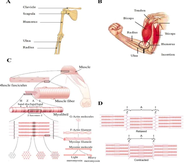
Skeletal muscles are attached to the skeleton. They are anchored by tendons to two bony structures which are linked by an articulation. The upper limb for instance has two main articulations one at the shoulder level and one between the arm and the forearm. This is illustrated in Fig 2.1A where the humerus of the upper arm is attached to the skeleton through the scapula articulation which is an element of the shoulder. The lower end of the humerus makes an articulation with the ulna and radius. Those two bones of the forearm permit many movements that can be produced by the hand. As shown in Fig 2.1B, the biceps brachii is attached at the shoulder and elbow level and when this muscle is contracted, a flexion at the elbow level is produced. To produce an opposite movement, another muscle, the triceps (also seen in Fig 2.1B) is attached across the elbow articulation but in opposite direction has to be contracted.
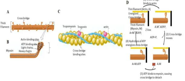
A muscle is composed of many fibers which are generally aligned in parallel. Those fibers (Fig 2.1C) are bundled in groups called fascicles and a muscle is composed of several fascicles. Looking closely at a muscle fiber, it can be seen that it is made of many subunits called myofibrils. When a myofibril is examined, a repetition of zones of different intensities separated by vertical lines is seen all along its length. Called sarcomeres, those repeating units, are each shortened during a muscle contraction by a micron or so. The sum of each of those microscopic shortenings results in an appreciable change in length of the contracted muscle or in a production of a force. Sarcomeres are made of thin filaments of actin and of thick filaments of myosin which are intermingled as can be seen at the bottom of Fig 2.1C. When those filaments slides between each other during a contraction, their length is reduced (Fig 2.1D).
2.1.2 Physiology
To produce a voluntary movement, a command is generated in the brain and communication between its neurons and the peripheral muscles is done through action potentials (APs) which are
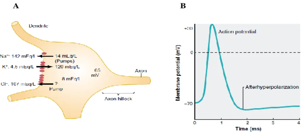
produced within each of those neurons and muscular fibers. At rest, the potential inside a cell is around -65 to -70 mV due to its semipermeable membrane and the ionic gradients existing between the interior and the outside (Fig 2.2A). When few sodium (Na+) ions are moved inside the cell due to an input to its dendrites, a depolarization occurs while a hyperpolarization is induced when potassium (K+) ions leak out of the cell. When the depolarization is important enough to reach a certain threshold, an all or nothing phenomena occurs (Fig 2.2B): a massive number of Na+ ions flow in the cell causing an important depolarization reaching momentarily ~+20 mV following which an important amount of K+ ions flow out of the cell and repolarize it. After a rapid passage below the resting potential the resting potential is re-established.
Fig 2.1 A. Bones of the arm attached to the shoulder articulation (Encyclopedia Britannica Online). B. Transverse view of the arm with anatomical position of the biceps and triceps (from [7], p. 156). C. Structure and components of a squelettal muscle up to a sarcomere within which item F represents a section of an actin filament, G a section of myosin, H a section in the middle of the sarcomere and I a section where actin and myosin can interact D: Illustration of the shortening of 3 sarcomeres (from [22], p.74-75). Muscle Muscle fiber Muscle fasciculus H band Z disc A band I band Z Sarcomere Z Myofibril G-Actin molecules F-Actin filament Myosine filament Myosine molecule Light meromyosin Heavy meromyosin
Fig 2.2 A: Schematic of a neuron where the different concentrations of Na+ and K+ across its semipermeable membrane create a
resting potential around -65 Mv (from [22], p. 564) B: when dendrite activity causes a depolarization high enough to reach a thresholed, an action potential is generated (from [58], p. 191).
APs generated in the brain to produce a movement are propagated by their axons in the spinal cord where they are grouped within nerves to finally make contact with the motoneurons (MNs) (Fig 2.3). Axons of the MNs leave the spinal cord to reach a muscle, when near a muscle each axon of a MN produces many branches each of them making contact with a different muscle fiber. A motoneuron plus the fibers to which it is connected constitute a motor unit (MU). The number of MUs per muscle in humans may range from about 100 for a small hand muscle to 1000 or more for large powerful limb muscles [35]. An example of a MN making contact with 2 muscle fibers and a second one which makes contact with 3 other muscular fibers is illustrated in Fig 2.3. Activity in a MN induces the contraction in all the muscle fibers to which it is in contact.
Fig 2.3 Axons of 2 motoneurons extending from the spinal cord to a muscle. Each axon divides into a number of branches that make contact with some of the muscle fibers scattered throughout the muscle (from [35], p. 251).
2.1.3 The Neuromuscular Junction and Mechanisms of the contraction
Where 2 muscular APs are produced, each travels in opposite direction up to the 2 tendons. As those 2 APs move along the fiber, they also propagate in the transverse (T) tubules which are surrounding the sarcoplasmic reticulum which encircles each myofibril (Fig 2.4). In the transverse tubules, the passage of the AP induces a Ca++ release from the lateral sacs of the sarcoplasmic reticulum. As previously mentioned, myofibrils are made of actin and myosin. In Fig 2.5A, myosin is represented by two large polypeptide chains with cross-bridges pointing toward the thin filaments (Fig 2.5B). The thin filaments also contain two other proteins: troponin and tropomyosin (Fig 2.5C). At rest, the cross bridges are not in contact with the actin but when Ca++ is present, it removes the troponin-tropomyosin complex from the actin making possible the interaction of the myosin cross-bridges with actin. This leads to the sliding of the actin over myosin filaments and consequently, the contraction of each sarcomere of each myofibril (Fig 2.5D). As long as Ca++ ions are present, the process is repeated again and again until the actin filaments pull the Z membrane up against the ends of the myosin filaments or until the load on the muscle becomes too great for further pulling to occur. When no more APs from the motoneuron are reaching the end-plates, the Ca++ ions are pumped back in the sarcoplasmic reticulum and the sarcomeres regain their initial length and are ready to contract again.
2.1.5. Two types of contractions
In an isotonic contraction, the tension generated in the muscle remains constant throughout the contraction while the muscle length is modified (Fig 2.6A). .In an isometric contraction, a force is produced while the muscle length is kept constant (Fig 2.6B).
2.1.6. Recruitment of MUs
The force generated by a muscle is proportional to the number of active MNs and the number of fibers they innervated. There are three types of MUs:
1- Slow (S) which innervate a small number of small fibers,
3- Fast-Fatigable (FF) which innervate a large numbers of fibers of large size.
Fig 2.4 Anatomic structures of the transverse tubules and of the sarcoplasmic reticulum system in a single skeletal-muscle fiber (from [58], p. 303).
For the S type, force production is due to an oxidative process which relies on the presence of oxygen and the force produced is small. For FFR type, energy to contract is partly dependent on the availability of oxygen and on the presence of stored glycogen within the fibers. Those MUs produce a greater force than S units, Finally, FF fibers are only using the glycolytic process for its energy source and their force output is large.
For a contraction of low intensity, the S (also called type I) MUs are activated. When more force has to be produced, additional S MUs are recruited as well as those of type FFR (or type IIA). When still additional force is needed, FF MUs are then added to S and FFR types (Fig 7A). This order of recruitment from the smaller to the larger MUs (i.e. S to FF) is named the Henneman principle (Fig 2.7B). The largest MUs are thus set in action in only few occasions. As seen at the bottom of Fig 2.7A, when a MU of type S is solicited on a long period of many minutes, its mechanical output is kept constant and such MU is said resistant to fatigue. When a FFR unit is solicited for a long time, fatigue sets in and its produced force decreases with time. The presence
of fatigue develops more rapidly for the powerful FF units. This is due to the differences between the oxidative and the glycolytic processes used by those MUs to produce energy.
Fig 2.5 A: Heavy chains of myosin molecules form the core of a thick filament. The myosin molecules are oriented in opposite directions in either half of the filament. B: The two globular heads of each myosin molecule extend from the sides of the filament forming a cross bridge. C: A molecule of troponin is bounded to a molecule of tropomyosin and that association prevents interaction with the myosin cross bridges. D: Four stages of a cross-bridge cycle. 1: In presence of Ca++, a link is made between
actin and myosin. 2: the binding triggers the release of ATP which induces an angular movement of each crossbridge. 3: A new ATP binds to the cross bridge and cause detachment from the actin. 4: ATP is splited into ADP and P for new movement. M* represents an energized myosin cross bridge (from [58], p. 299, 300, 302).
Fig 2.6 At the left, the load pulling on the muscle is constant and an isotonic contraction is produced when the muscle is stimulated. At the right, the length of muscle is kept constant and an isometric contraction is produced (from [22], p. 80).
Fig. 2.7 A: three types of motor units with the amplitude of their twitch when electrically stimulated and their resistance to fatigue upon continuous stimulation.B: The size or Henneman principle: small motor units are initially recruited and when more power is required to increase the speed, medium and large MUs are then recruited (from [41], p. 451).
2.1.7 Muscle compartments
Generally, muscles are considered as single entities but this not always the case. For instance, the dissection of the cat lateral gastrocnemius muscle was revealed four compartments each innervated by a primary branch of a nerve. Activity within each compartment was collected with implanted electrodes and when the cats walked at low speed, more intense EMG activity was found in distal than proximal compartments while at moderate to fast speeds, the intensity of activity in proximal compartments was equal to or greater than in the distal compartments [5, 9, 10 and 31].
As for the human biceps brachii (BB) muscle, dissections of Segal [51] revealed on the dorsal face of the muscle the presence of 4 to 8 (Fig 2.8) natural grouping of the fibers called
compartments. Each of those grouping is innervated by a nerve branch which sometimes gave other branches suggesting the presence of smaller units within a compartment. Electrophysiologically, Ter haar Romeny et al ([53], [54]) reported for the cat LG muscle, that the territory of a MU occupies only a fraction of the muscle cross-section area. This factor, coupled with the broad tendons linking the muscle to the bones, lead to its implication in the production of different movements of the cat upper-limb ([60], [61]).
For English et al. [11], the ramification of each compartment nerve branches is a significant aspect of muscles control to consider since in a compartment, a nerve can be divided in primary or first-order nerve branches which could divide to produce other (higher order) branches. In the primary nerve branch, motoneuron axons enters only one compartment while for the higher nerve branches, the axons of some MNs can innervated several compartment sub-units called subcompartments (Fig 2.9). Beside the BB, neuromuscular compartments have also been observed in other human arm muscles such as the flexor carpi radialis and the extensor carpi radialis longus [52]. Ability of voluntarily contracting those compartments individually or in groups could be very useful to facilitate the control of myoelectric prostheses by amputee persons.
Fig. 2.8. Posterior view of the biceps brachii where asterisks indicate neuromuscular compartments in the long and short head. In the most cases, musculocutaneous nerve does not insert to the long and short head of BB directly but it divided into several branches each * identifies a compartment. (from [51], p.100).
Fig 2.9 Schematic representation of motoneurons and compartments of one muscle. The circles at the top of the figure represent the motoneurons innervating a muscle, and the boxes at the bottom symbolize the different compartments of the muscle innervated by these motoneurons. Each compartment is illustrated by different shades. Each motoneuron is connected to its compartment by axon which is demonstrated by one solid line. The collection of axons into a single muscle nerve and the branching of this muscle nerve are indicated by the horizontal dashed lines. (from [11], p. 861).
2.2 EMG recording techniques
2.2.1 Intramuscular electrodes
The ionic exchanges associated to the initiation and propagation of an AP within muscle fibers give rise to electrical potentials called electromyograms (EMG). To record that signal, fine electrodes of various types can be inserted inside a muscle. For example, when inserted in a muscle, the concentric and monopolar needle electrodes which have a small recording area (~0.20 mm2) can be used to record the activity of only few muscle fibers of a given MU which are in its close vicinity (Fig 2.10). Amplitude of the recorded signal is proportional the electrode uptake area: with large recording surfaces, activity from a large area within the muscle is picked up. A large amplitude signal with a reduced spatial selectivity is thus obtained.
Fig. 2.10 Illustration of a concentric needle electrode inserted close to the muscular fibers of 3 MUs which are simultaneously generating an extracellular APs with amplitude proportional to the diameter of the MU’s fibers. Activity of the closest fibers to the electrode will have the largest contribution to the signal collected. In the illustration, activity of the top MU will be first detected because its neuromuscular end-plate zone is closest to the electrode. (from [36] p. 29)
2.2.2 Surface electrodes
Intramuscular recordings are invasive and thus used in special settings when information collected is greater than the risks associated with the procedure. Surface recording where electrodes are directly placed on the skin surface is thus the most frequent method of collecting EMG signals. The diameter of surface electrodes can vary from 4 to 10 mm and are usually made of Ag/AgCl, or with silver or gold. The biological tissues interposed between the surface electrode and the active fibers constitute a volume conductor which acts as a low-pass filter.
Surface electrodes can take different configurations (Fig 2.11A). When spatial sampling of the activity over a muscle is of interest, linear or a matrix array of electrodes can be used (Fig 2.11B and C).
Signals at the electrodes level may be in the microvolt (µV) range and should be amplified by a factor of 1000 or more. Amplifiers need to have high input impedance, a high Common Mode Rejection Ratio (CMRR) and have a low noise level. Analog filters can cover 2 Hz to many KHz. Monopolar recording (Fig 2.12A), bipolar (single differential (SD) and double differential (DD) (Fig 2.12B, C) is possible. Bipolar or differential (SD configuration is most frequently used due to its interferences removing such as power line [2]. DD configuration is used when crosstalk originating from other muscles is to be minimized and for non-invasive conduction velocity measurements [20].
Fig. 2.11 A. Surface electrodes and surface EMG signal over the BB with the arm abducted and a weight at the wrist corresponding to 20% of maximal voluntary contraction. B. Linear array combination of surface electrodes (from [36], p.181). C. an electrode array of 3 x 8 electrodes used to collect signals around the arm as used in [8].
Fig. 2.12 Different recording of EMG signals A. Monopolar B. Single differential (SD) C. Double differential (DD) (from [3], p.181)
2.3 Direct Problem
Relatively few activities have been carried on the direct and inverse problem in the EMG field as compared to ECG and EEG. However, since the generation of those 3 signals have similar electrophysiological basis, the approaches used in ECG and EEG can thus be of great help for the EMG situation. A pioneer in the field, Plonsey [45] produced in 1977 a tutorial paper where he quantitatively described how, in cylindrical nerve or muscle fiber; the extracellular field are related to the underlying current sources.
Electrode signal Ground Output Vcc Ground + -Electrode signal Output1 Vcc Ground + -Electrode signal Output2 + -+ -+ -Electrode signal Vcc Ground + -Electrode signal + -+ -Output Vcc Ground + -+ -A B C A B C 0 1 2 3 4 5 -0.6 -0.2 0 0.2 0.6 EM G am plitu de (m V) Time(s)
At that time, only simple characteristics of the medium through which the signal propagates (volume conductor) where considered (i.e. unbounded, homogeneous, and isotropic). Spheres where initially used as a representation of the heart and the head but since the ECG signals were collected on the torso, the cylinder appeared as a more realistic shape. Cylinders without top and bottom (unbounded) or with top and bottom (bounded) where then considered (Burger et al [4]). It is within that context that Frank [16] conducted experiments with a tank filled with a conductive medium in which a dipole representing the heart was placed on or off the cylinder’s axis. Modeling an infinite cylinder, he obtained a good match between the theoretical results and the experimental data. Efforts were also directed at solving the equations used in those models. For instance, Okada [42] developed a simpler computational method than Burger [4] and got similar results. As for Lambin and Troquet [30], they solved, with the Green’s function, the Poisson’s equation for a dipole positioned anywhere within a finite length cylinder filled with an homogeneous medium.
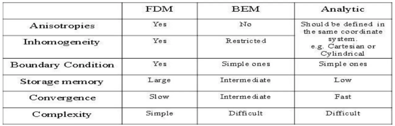
With computer availability, various numerical approaches were developed to facilitate the solution of the equations of Laplace and Poisson. To evaluate the available methods for the forward problem, Heringa et al. [26] compared the finite difference method, the discretized integral equation method and the analytic method when applied to a source distributed along the axis of a bounded cylinder filled with an homogeneous medium. Advantages and disadvantages of the 3 methods considered are presented in Table 2.1.
Table 2.1. Comparison between the finite difference method (FDM), the discretized integral method called boundary element method (BEM) and the analytic one (Analytic). (from [26], Table 1)
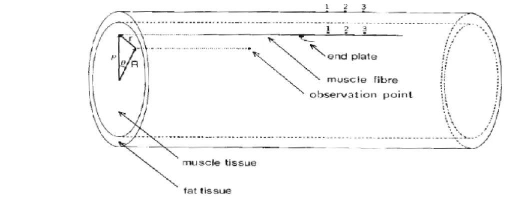
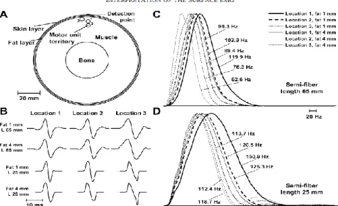
Effect of a finite limb dimension within which muscles have a finite length on the modelisation of motor unit action potentials (MUAPs) was studied by Gootzen et al. [18]. They used an analytical method and their volume conductor consisted of an inner compartment representing a resistive anisotropic muscle, an outer less conductive isotropic compartment to model the subcutaneous fat tissue and finally air is all around this volume conductor (Fig 2.13). Their results indicate that for a good simulation of MUAPs that can be detected at an increasing distance from the skin surface, considering a finite limb and muscle dimensions is a necessity. Trying to model EMG data collected over the BB with a two compartments model, Blok et al [1] found inconsistencies which prompt them to add a third layer to represent skin tissue (Fig 2.14A) In an homogeneous and isotropic volume conductor, they simulated the effect of increasing fiber
Fig. 2.13 Two concentric cylinders of finite dimensions to model singlr fiber extracellular action potential. Inner cylinder represents the muscle tissue considered anisotropic, Outer cylinder to model the fat layer is isotropic (from [18], p. 153).
depth on the potential at the skin surface. As shown in Fig 2.14B, the downward wave at the end of the simulated signals represents the effect of the tendon when the active fiber is located deep in the volume conductor. When the fiber is near the surface, its propagating signal is large and the effect of the tendon is then barely visible. In Fig 2.14C, by comparing the MF and M curves, it can be seen that the fat layer contributes to the increase of the potential amplitude and reduces its width. The opposite effect happens for the effect of the skin tissue which reduces the amplitude and increases its width. The combined effect of fat and skin thus depends on the relative thickness and conductibility of each layer. Using the 3 layers model, they found that the rate of amplitude decline over the circumference of the cylinder with increasing source depth was similar for both the experimental data and the simulated signals (results not shown).
Fig 2.14 A: Three concentric cylinders simulating muscle tissue, fat and skin layer. The inner cylinder represents the anisotropic muscle the middle one the fat and the third one the skin both considered isotropic. R represents the distance of an active fiber from the center of the model and r the distance between the fiber and the surface of the model. ϕ is the angle between the active fiber and the point of measurement and ρ is the radius to the skin surface. In the longitudinal view, a is radial distance of the active fiber. b is the radial distance to the upper limit of the fat layer and c (equal to ρ) is the distance to the skin. The source is represented by the horizontal fiber with its neuromuscular junction at its center. B: Simulated signals when the active fiber is placed at various depth (FD) in an homogeneous volume conductor. The downward peaks (to the right of the signals) are associated to the effect when the AP reaches the tendon. C: Simulation results for a motor unit composed of 300 fibers at a depth of 5 mm under the skin when the volume conductor is considered to be composed of only an anisotropic muscle compartment (M), of a two-layered model of muscle and fat (MF) or muscle and skin (MS) and for a three layered model (MFS); (from [1], Fig.1, 2 and 3).
For Farina et al. [14], air surrounding a limb is considered as a fourth layer to be added to muscle tissue, fat and skin layers. They then calculated the potential distribution over the skin, due to sources in the muscle by solving the Poisson equation in the spatial frequency domain. The model is based on a cascade of low-pass spatial filters representing the anisotropic muscle tissue and the isotropic fat and skin layers. The results illustrated the effect of the sub-cutaneous tissue layers increase the detection volume in all directions and reduced its amplitude (Fig 2.15). To compensate the attenuation and widening of the signal due to the subcutaneous tissue, various recording electrode arrays such as shown in Fig 2.16A could be used. The transfer functions of anisotropic muscle tissue and the isotropic layers of fat and skin is shown in Fig 2.16B.
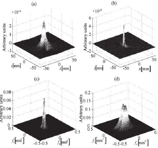
Fig. 2.15. Spatial and spatial frequency domain potential distributions at the skin surface (a and c) and directly over the muscle (b and d) as generated by a fiber located at 2 mm under the skin Simulated thickness of 3 and 1 mm was respectively used for the fat and skin layers, A current tripole with wirh a length of 7 mm represented the depolarized zone of the fibers. (from [14], Fig.3),
Fig 2.16. A: Structure of a spatial electrode matrix. The weights of the filled circles were varied according different filters and the weights of white circle were zero. B: Block diagram of anisotropic tissue and isotropic tissue (fat and skin). (from [14],Fig 2 and 8).
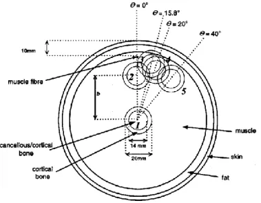
Pursuing on how the modeling of the volume conductor interacts with spatial filters, Farina et al. [13] studied the spatial selectivity offered by various electrodes configurations in order to separated pr opagating (APs travelling in muscle fibers) and non-propagating signals (generation of the APs at the neuromuscular junction and their extinction at the tendons). They considered 3 different anatomical configurations as shown in Fig. 2.17a. In b of that figure, a lateral view of the volume conductor with a finite-length muscle fiber placed near the detection surface at a position located between the end-plate (neuromuscular junction) and the tendons. As shown in Fig.2. 17c, three different spatial filters where considered: the longitudinal single (LSD), double (LDD) and normal double differential (Laplacian, NDD). By combining those spatial filters and various thicknesses, 13 different configurations were analyzed with an analytical model simulating the generation, propagation and extinction of an IAP within the muscle fiber. Effects of the configuration of the electrodes on the transverse selectivity (around the cylinder away from the electrodes) and on the depth selectivity (effect of the depth of the active fiber) were considered.
Fig. 2.17.Volume conductor models with bone-muscle, bone-muscle-fat, and bone-muscle-fat-skin. b. Lateral view of the volume conductor with simulated finite-length muscle fibre which varied between 30 and 50 mm. The detection point represents the position of the middle electrode of LSD, LDD and NDD. It is positioned in the middle between the end-plate and a tendon. c. Configurations of 3 filters with their associated weights for each electrode. (from [13], Fig 1).
Fig 2.18 Transverse selectivity (TS) between peak-to-peak amplitude of signals generated by the muscle fiber at 0 ° and 10 ° in the transverse direction relative to the detection system as simulated in different anatomical conditions. The muscle fiber is simulated with a 50 mm length and at a depth of 1 mm in the muscle Moreover the inclination angle between muscle fiber and detection system was 0 ° or 15 °. b. TS when length of fiber was 30 mm. ( ) NDD; ( ) LSD; ( ) LDD. ( ) NDD, 15 ° of misalignment; ( ) LSD, 15 ° of misalignment; ( ) LDD, 15 ° of misalignment. (from [13], Fig 5).
In Fig.2.18, results indicate that propagating as well as non-propagating signal components are highly influenced by the model considered. LSD, LDD and NDD show similar performance with some anatomies (e.g. when the fat and skin was not considered), whereas they perform significantly differently with other situations. When the radius of bone, muscle, fat and skin layers were assumed to be 20, 28 and 1mm respectively, by increasing the lateral displacement of the detection system from 0° to 10°, the propagating components are approximately reduced to 2% with LSD and LDD and to 4% with NDD. By increasing the fat layer to 5 mm and reducing the muscle to 24 mm, LSD and LDD reduce the signal amplitude to approximately 25% and 20% respectively, whereas, with NDD, amplitude decreases to 4%.
As expected, when isotropic layers of fat and skin are added, there is a decrease in selectivity in propagation component. For the nonpropagation components, NDD is generally less selective than LDD and LSD but the importance of the difference depends on the anatomy model considered. For the propagation components, LSD and LDD may be more or less selective than NDD depends again on the volume conductor model. In an article aimed at extracting neural strategies from surface EMG, Farina et al. [12] surveyed the various factors which can affect the
features of the surface EMG signal. Among those shown in Table 2.2 crosstalk which is contamination of a signal recorded over one muscle by those generated by other nearby muscle(s), can be significantly reduced by the spatial filtering made by an electrodes configuration.
Table 2.2. Factors that influence the surface EMG (from [12], Table 2)
While simulation results indicate that LSD or LDD spatial filter would be more transversely sensitive than NDD, the inverse had been reported from experiments on some muscles among which the biceps is found [12].
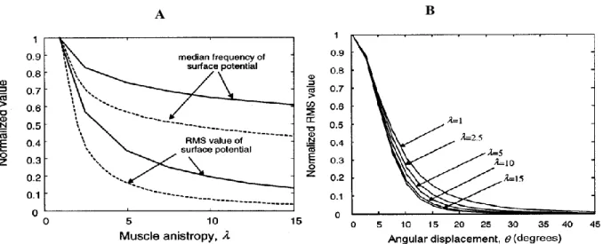
In a review article on the relation between physiological processes and surface EMG Farina et al. [14] used a 4 layers model (Fig 2.19A) to simulate for the upper limb, the effects of 2 muscle
lengths and two fat thicknesses on the surface signal characteristics. As illustrated in Fig 2.19B and C, the peak value of the power spectrum is shifted to lower values as fat thickness increased and when position of the source is changed relative to the detection point. In panel D, the same conditions as in C is shown except that the fiber length is shorter which results in broader spectra because of the prevalence of non propagating components. However, mean frequency decreases as the depth of the source is increased.
Fig. 2.19 A: Simulation of single MUAP measured with a pair of electrodes placed between the innervation zone and a tendon. The MU was placed in 3 positions within the muscle and occupies a circular territory (radius of 2 mm). It innervated 250 fibers with a density of 20 fibers/mm2. Locations 1 and 2 were at the same distance from the detection point, whereas location 3 was 4
mm deeper. Four conditions were considered: semi-fiber length of 65 and 25 mm and fat thickness layers of 1 and 4 mm. Conduction velocity was 4 m/s. B: Changes in MU potential waveform (normalized maximum values) due to the influence of fiber depth, fat thickness and fiber length. C and .D: Power spectral densities of the MUAPs in different conditions. The bandwidth of the power spectrum was broader for shorter fibers (D vs. C). The distance from the detection system is not the only parameter to influence the power spectrum, for example, the power spectra at locations 1 and 2 are different. The depth of the source may decrease the mean frequency which may increase for large distances, especially when the fibers are short, because of the prevalence of nonpropagating components. Despite a constant conduction velocity, the frequency bandwidths were significantly different in the 12 cases (2 fiber lengths from 50 to 130 mm, 3 locations of MU 2 fat thicknesses from 1 to 4 mm). (from [14]. Fig 5).
Considering that surface EMG models do not take into consideration that the volume conductor is not space invariant, Mesin et al [37] introduced spheres of different conductivities in the volume conductor. With an analytical solution, they found that the spheres modified the signal propagation (Fig 2.20) and reduced the amplitude of the detected signals
Fig.2.20 Insertion of a circular inhomogeneity in an otherwise homogeneous volume conductor perturb the surface potential. a) Perturbation (small amplitude wiggles) on the impulse response associated when the source is at 2 different locations. b) Signal associated of the impulse current source alone (1/s) and with the perturbation induced by the sphere (A.n/(s-sp)2) where A is
related to the conductivity in each axis of the sphere. Perturbation effect decays rapidly as the distance from the inhomogeneity is increased C) Contours of the perturbation effect for 3 positions of the current source (from [37], Fig 1).
The effects of the presence of the homogeneity at 2 positions relative to the detection point (Fig 2.21a) on the surface signal detected with 4 different electrode configurations (Fig 2.21b) is shown in Fig 2.21c. The results show that sensitivity to the presence of the sphere depends on its location and to the electrodes configuration. Those results indicate that homogeneities has to be considered when elaborated volume conductors are considered but the perturbation effect of inhomogeneities decreases as the inverse of the square of the distance from the detection point. It has also to be noted that the perturbation travels on the signal in opposite direction to the direction of the propagating source.
![Fig 2.4 Anatomic structures of the transverse tubules and of the sarcoplasmic reticulum system in a single skeletal-muscle fiber (from [58], p](https://thumb-eu.123doks.com/thumbv2/123doknet/2338021.33278/26.918.195.679.171.500/anatomic-structures-transverse-tubules-sarcoplasmic-reticulum-single-skeletal.webp)