The Correction of Chronologic Series’ Seasonal Fluctuations
T
HE
C
ORRECTION OF
C
HRONOLOGIC
S
ERIES
’ S
EASONAL
F
LUCTUATIONS
ACCORDING TO
S
EASONAL
S
IMULTANEOUS
A
DDITIVE AND
M
ULTIPLICATIVE
E
FFECTS
R. BOURBONNAIS* Ph. VALLIN**
A
bstract
In this study, we set the problem of the probable existence of an additive and multiplicative mixed seasonality. In this context, we show by some simulation that the seasonality correction according to a pure additive or a pure multiplicative scheme leads to biased estimators of the coefficients and, consequently, of the calculation of seasonally adjusted series which is necessary for quantitative demand analysis. The use of an analytical resolution technique allowing simultaneous estimation of the trend coefficients and the additive and multiplicative seasonal coefficients works perfectly if the series is affected by a simple linear trend. In this case, the estimation gives the theoretical seasonal coefficients.
An application study to the mobile phone market, the new product split in two markets, professional and individuals, allows evaluating the contribution of the methodology. Keywords: seasonality, demand analysis, time series.
JEL Classification: C32, C12
The study of the chronological series’ seasonality is a prerequisite for the quantitative analysis of demand. When this effect exists, it is convenient to filter it before being able to analyze the other characteristics, such as: the trend, the impact of marketing
* EURISCO, University of Paris-Dauphine, Place du Maréchal de Lattre de Tassigny, 75775
Paris Cedex 16, [email protected].
** LAMSADE, University of Paris-Dauphine, Place du Maréchal de Lattre de Tassigny, 75775
Paris Cedex 16, [email protected].
mix activities, etc. This allows estimating the real effects of the factors that structure the demand.
In general, this filtration proves to be indispensable because, in most of the cases, the scope of seasonal effect masks the impact of the other characteristics. The objective of this article is to point out that if a chronological series is not the achievement of a justifiable process of a decompounded scheme purely additive or purely multiplicative, then the traditional methods of eliminating seasonality are weak. That is because, as a general rule of analyzing chronologic series, one or the other is applied after having determined the most suitable decompounded scheme.
If the major part of macroeconomic series is known for long periods of time, it is not the same thing at the microeconomic level. The products’ life being shorter and shorter, companies possess sales archives over four, five years or more. The software packages for forecasting sales most often used by companies, by default, appeal to a multiplicative scheme, this without any justification! We think that in reality, expressing the demand is rarely – at least there is no reason – the result of a pure decompounded scheme.
We consider particularly:
• the enterprises addressing to several markets, a public market and an industrial market. The public market is able to develop when the industrial market is able to remain stable, the two markets having their own proper seasonality; for example, the glue from paintings who interferes in the industry and DIY, and the selling of liquefied petroleum gas delivered to households and industries. Of course, in certain cases, it is possible to segment the markets, but this is not always achievable (the absence of statistics) or desirable (because of the substitution between products). For example, the production of certain electronic compilations may have as final destination the equipments consumed on different markets of very different types, without the producer of compilations being able to have the basic information about the filter which is represented by distributors.
• the “innovatory” behavior scheme, a person rapidly buying a new product, proposed by Midgley et Dowling (1978) and presented by G. Roehrich (2001). In this scheme, two populations having different buying behaviors may coexist: one of people with a very innovative attitude, having received very favorable information about the product, and the other, less innovative but more concerned about the category of products, which is in a favorable buying situation. In this case, the seasonal impact will have a component proportional to the level of sales linked to the dissemination of information to the first population and a constant component generated by the second population.
Starting with simulations, we try to demonstrate that using a mixed decompounded scheme over a short data history gives better results, in other words, a better filtration of seasonality than the additive or multiplicative eliminating of seasonality. This improvement of filtration thus allows for a more refined analysis of the other characteristics of demand and, as a result, a better forecast.
After that, with the help of an analytic resolution of a mixed theoretical scheme, we find the seasonal coefficients of the generated records.
The Correction of Chronologic Series’ Seasonal Fluctuations
Finally, an application on the mobile phone market, an innovative product segmented in two markets, professionals and individuals, allows for the evaluation of the interest in this methodology.
2
.
Choosing the decompounded scheme
2.1. Definition of schemes
It does not exist a perfectly satisfying method for estimating seasonal coefficients: any method we choose, the risk of incorporating fluctuations owed to erratic values (called aberrant or abnormal values) in seasonality is always present. At the moment of calculating the seasonality, it is suitable to do a certain number of choices regarding the type of seasonal coefficients (additive/multiplicative, fixed/slipping), choices which we shall present. The estimated values of the seasonal coefficients are different, depending on the methodology used.
The seasonality of data series may sometimes be influenced by the extra season of/and the residual component. Given the existence of these interactions, there were derived the decompounded schemes of chronological series: additive, multiplicative or complete multiplicative.
- The additive scheme which supposes the orthogonality (independence). It is written as follows: xt = Tt + St + Rt . In this scheme, seasonality is rigid in amplitude and in
period.
- The multiplicative scheme: xt = Tt× St + Rt , in which the seasonal component is
linked to the extra season (flexible seasonality with the variance of amplitude proportional to trend).
- The complete multiplicative scheme: xt = Tt × St × Rt in which the seasonal
component is linked to the extra season (seasonality and the residual component are flexible with the variance of amplitude, in time). Currently, it is the most used in the area of sales forecasting.
Thus, the idea is to compare three methods for eliminating seasonality on the basis of three schemes:
• an additive scheme; • a multiplicative scheme;
• a mixed scheme, integrating additive and multiplicative seasonal coefficients. We present two simple techniques, the first one empirical, for selecting the scheme.
2.2. The band test
The “band test” consists in starting from the graphic of raw series’ evolution and connecting by a shattered line all the “upward” and all the “downward” values of the chronological series. If, on the visual exam the two lines seem parallel, the decomposition of the chronological series can be achieved according to an additive
scheme; in the opposite case, the multiplicative scheme seems more suitable. Figure 1 and Figure 2 show an interpretation of the band test.
Figure 1
Exemple of additive scheme
Figure 2 Exemple of multiplicative scheme
2.3. The Buys-Ballot test
The Buys-Ballot test (cf. Bourbonnais R. et Terraza M., 2004) is based on the results of calculating for every year the means and gaps types of the raw series. The scheme is, by definition, additive if the type of gap and the average are independent; in the opposite case, it is multiplicative. When the number of years is large enough, one may estimate using the method of Least Ordinary Squares (MCO), the parameters of the equation: a1 and a0
The Correction of Chronologic Series’ Seasonal Fluctuations σi = a1
x
i + a0 + εi .σi = the type of gap of cases in the year i,
x
i = the average of cases in the year i,i = 1, N (N = the number of years).
In the case when the coefficient a1 is not significantly different from 0 (the Student
test) we accept the hypothesis of an additive scheme; in the opposite case, we reject the additive scheme and, simplifying, we choose the multiplicative scheme.
These two tests sometimes lead to ambiguous results. This is the reason why the majority of authors recommend the use of a multiplicative scheme. Moreover, when the economic phenomenon is observed over a long period of time the structure of the series often changes, passing from an additive scheme to a multiplicative one. It is thus convenient, not to confuse the historical period with the number of observations: it is possible to have many observations over a short period (the continuous stockexchange quotations) when the structure of the series remains stable.
2.4. Fixed or slipping coefficients?
We are also facing the choice of estimating fixed or slipping seasonal coefficients: • Fixed coefficients: the coefficients calculated are the same whatever the
analyzed year.
• Slipping coefficients: the coefficients evolve every year.
A seasonal movement is repetitive every year and it has to repeat similarly. It seems thus improper to calculate different coefficients every year. However, in certain circumstances, in which a marketing reflection suggests an evolution of behaviors, it may be interesting to integrate a slipping seasonality.
Calculating a coefficient for every month, the risk of incorporating a piece of “noise” in seasonality intensifies. In fact, the distinction between seasonality and the residual component will be more difficult to be done in the absence of a rigidity constraint of the seasonal coefficients. For example, if due to weather reasons, a year was particularly favorable to the beer consumption, a slipping seasonality will reflect this seasonality in the next year without any a priori reason, without knowing the temperature in advance. In this case, a multiplicative fixed seasonality imposes.
A contrario, a risk deserves to be pointed out: the possible confusion between the real seasonality and a fictional seasonality created by the company. It regards the companies making promotions or tariff variances in the same period each year. The calculation of the seasonal coefficients attributes to seasonality these “supra – sales” owed to the voluntary politicies of the firm. A problem rises thus when the company modifies the date of promotions. In this case, using slipping seasonal coefficients allows integrating this modification more rapidly.
Except for the marketing reflections motivating a predicted evolution or modification in the habits of consumers, the fixed seasonal coefficients are generally used.
3
. The methods of eliminating seasonality
When a chronological series is structured by seasonality, the intertemporal comparisons of the phenomenon need a series Corrected for Seasonal Variances, written down as CVS.
The seasonality of the sale of an article conceals the true evolution of sales; the sales
of a raw series are not thus able to be interpreted.
In addition, it is easier to forecast sales without the seasonal phenomena: • the “real” trend can be calculated;
• the real impact of the explanatory factors (publicity, promotions, etc.) can be pointed out.
Eliminating seasonality from a chronological series is eliminating seasonality without modifying the other components of the series. It is a delicate operation, a fact that explains the great number of methods for eliminating seasonality. The most used, for macroeconomic series, is the method of CENSUS. However, it requires historical data over long periods of time, up to 10 years.
The choice of the most appropriate technique depends on the deterministic or random (stochastic) nature of the seasonality of series:
• when it is deterministic (in other words, rigid, well-marked and repetitive) the methods of regression and the usage of seasonal coefficients identical over the historic period are adapted;
• when it is random (the coefficients are affected by a random term) the techniques of filtration by moving averages (CENSUS, for example) must be used.
The preservation of ranges principle
The analysis of seasonality has as target a new distribution of the “intra-annual” profile of the series without modifying the level achieved by annual cumulus: the annual averages of the raw and CVS series have to be identical. Standardization allows calculating definite seasonal coefficients.
The CENSUS method
Eliminating seasonality by using simple moving average is often insufficient because of various reasons (fluctuating seasonality, extra complex seasonality). In 1954, Shiskin J. proposed a method of eliminating seasonality using in an iterative way multiple moving averages. As CENSUS methods are built starting from successive iterations of moving averages of different order to better apprehend the trend (Tt), as
well as the fluctuations of seasonality, they determine the loss of information at the final extremity of the series. This loss of information is contained by a Box and Jenkins type of forecast, before eliminating seasonality from the series, by a number of points equal to the inherent loss of information when using moving averages.
The Correction of Chronologic Series’ Seasonal Fluctuations
In the area of sales forecasting based on a short history, this method is, thus, inoperable.
The seasonal differences
Using the filter proposed by Box and Jenkins (1976) to seasonal differences in the form: (1 − Bp) x
t = xt – xt–p (p = seasonal period, p = 12 for a monthly series of annual
period) allows for making stationary a series influenced by a seasonal movement. The tests of HEGY (Hylleberg, Engle, Granger, Yoo, 1990) and Franses (1990) use this type of filter with polinoms (1 – B4) for quarterly series and (1 – B12) for monthly series. The complexity of applying tests for the presence of seasonal unit root makes it impossible to use this approach in enterprises.
The method based on related to trend
This method is the one used by us; it is described in Section 4.1. In fact, in the context of an enterprise in which sales history is very well known over four years, the CENSUS method is inoperable. That is why we have chosen the method of estimating trend by moving averages and fixed coefficients, method which is the most used in enterprises.
4
. Methods of eliminating seasonality
The chronological series is composed of n cycles, each comprising p periods.
4.1. Method 1: Classic methods (pure additive scheme and pure multiplicative scheme)
Firstly, we proceed by two eliminations of seasonality following an additive scheme and a multiplicative scheme. The method of eliminating seasonality applied (cf. Bourbonnais R. and Usunier J. C. (2006), pages 42–51) is the most widespread in sales forecasting software packages, due to the short historical data series available in companies:
a) Estimation of trend by calculating centered moving averages over p=12 months (the case of an annual periodicity with monthly data). MMt is the average;
b) The calculation of xt / MMt ratio in the multiplicative scheme and the differences
xt – MMt in the additive scheme;
c) The seasonal ratios of coefficients are further on calculated by average on n – 1 years (the moving average does not allow for estimating the trend for the first 6 and the last 6 months);
d) At last, the seasonal coefficients, Sk, 1≤ k ≤ p; for the p periods of every cycle
are calculated for standardization in order to respect the principle of “preserving ranges”: • 0 1 =
∑
= p k A k S (additive scheme);• 1 1 =
∏
= p k M kS (multiplicative scheme); relation which is being used in practice
in the form: S p p k M k =
∑
=1, which is the alternative used here.
e) Thus, the series is without seasonality, due to these seasonal coefficients, thereby we obtain two series corrected for the seasonal values, obtained following the two schemes:
• following an additive scheme: CVSA t
x
• following a multiplicative scheme: CVSM t
x .
4.2. Method 2: The least squares estimators for the mixed scheme
We denote by:
n : number of cycles (of years) of common rank i,
p: the periodicity of series, number of periods (of common rank k) in the cycle, i : cycle rank ; i = 1, ..,n,
k: period rank; k =1, 2,…p: k= (t – 1 modulo p) + 1,
t: data rank, t=(i-1)p+k corresponding to the k period of the i cycle,
xt = xk i
: raw series at date t =(i-1)p+k corresponding to the k period of the i cycle,
Tt : value of the real trend at date t,
i k t
T
T
ˆ
=
: linear trend estimated at date t,M k
S
: seasonal fixed multiplicative coefficient associated to the k period,A k
S
: seasonal fixed additive coefficient associated to the k period,t
E
: residual component, the not explicated part of the series.The principle consists in determining simultaneously the roles of the seasonal coefficients M
k
S and A k
S by estimators, having in view the model mix.
Noting that if the trend is known (or estimated), the model is linear depending on seasonal coefficients, we can estimate seasonal coefficients Sk
M and S k
A (k = 1,2, …,
p) by least square estimators, solution of the linear classic system with 2 p unknown
and 2 p equations:
S = (A’A)-1A’X
The Correction of Chronologic Series’ Seasonal Fluctuations
X(np×1) : the xt column vector for n cycles of p successive periods,
⎥ ⎥ ⎥ ⎥ ⎥ ⎥ ⎦ ⎤ ⎢ ⎢ ⎢ ⎢ ⎢ ⎢ ⎣ ⎡ = n p i k x x x x X ... 1 1
X is composed by n underneath matrices associated to cycles i:
⎥ ⎥ ⎥ ⎦ ⎤ ⎢ ⎢ ⎢ ⎣ ⎡ = i p i i x x X ... 1 , i = 1…n.
S (2p×1): the column vector of components ⎥ ⎥ ⎦ ⎤ ⎢ ⎢ ⎣ ⎡ A k M k S S ; k = 1…p. A (np× 2p): the matrix ⎥ ⎥ ⎥ ⎥ ⎦ ⎤ ⎢ ⎢ ⎢ ⎢ ⎣ ⎡ I T I T I T n i 1 ; where i
T is the diagonal matrix, of order p, of
⎪⎭ ⎪ ⎬ ⎫ ⎪⎩ ⎪ ⎨ ⎧ i k T
elements for i cycle, k varying on p periods.
I is the unity matrix of order p.
A’ : A transposed.
E : column matrix of the residual components Et.
The estimators of Sk M and Sk A are:
( )
∑
∑
= = − − = n i k i k k k i k n i i k M k T n T x T n x T S 1 2 2 1 ˆ M k k k A kx
T
S
S
ˆ
=
−
ˆ
With∑
= = n i i k k T n T 1 1 and∑
= = n i i k k x n x 1 1 .We meet again the classic estimators of the linear model with an explanatory variable and a constant; here, the explanatory variable is the estimated trend at date t:
i k t
T
T
ˆ
=
. This result comes from the fact that the estimate of the seasonal coefficients is made by the resolution of p independent blocks of n equations.The basic model is: M A
E S S T
i k A k M k i k i k T S S E x = × + +
In matrix form, the system is written as follows: X = A S + E (1) Each square matrix T i
, i = 1, …n, of (p ×p) dimension, the form of component A is :
T i = ⎥ ⎥ ⎥ ⎦ ⎤ ⎢ ⎢ ⎢ ⎣ ⎡ i p i k i T T T 0 0 0 0 0 0 1
Thus, we return at p systems of n independent regression equations, each system k, 1≤ k ≤ p, being formed by n equations associated to n observations of the cycle of rank k comprising n periods, allowing for estimating the two parameters M
k
S and SkA
through the classic results of the two variables linear regression. The set of regression equations of system k is written as follows:
i k A k M k i k i k T S S E x = × + + , for i = 1,2, …n The second method:
If A’A is inversable, (this is especially the case if
Tˆ
t= a1 t + a0 with a1 ≠ 0), theseasonal coefficients estimators which minimize the square sum of residuals are the solution of the system: S=
(
A'A)
−1A'X (2);The subordinate diagonal matrix enables a relatively simple matrix calculation and the equality (2) provides the presented estimators.
This method of estimating seasonal coefficients allows for testing the “significance” of two types of coefficients, and thereby, for choosing one of the three models (multiplicative, additive and mixed). We provide in the next paragraph an estimation of the seasonal coefficients for four proposed series. The estimation of trend was made through a regression applied to the series of moving averages of order p = 12 in order to filter the seasonal influences.
5
. Artificial generating of data
In this section, we present the methodology used in order to make our simulations. We have generated over four years (48 monthly observations) monthly chronological series having a mixed decompounded scheme of the form:
(
)
A t M t t t T S S x = × + t = 1, …, 48. With:xt = simulated value of series at moment t,
The Correction of Chronologic Series’ Seasonal Fluctuations M
t
S = multiplicative fixed seasonal coefficients associated to the date t, S =tM StM+12
A t
S = additive fixed seasonal coefficients, S =tA A t
S+12
Intentionally, we have not added the hazard because the goal is to prove that a method not adapted (pure additive scheme and pure multiplicative scheme) does not allow for finding the real values of coefficients, whereas a mixed method allows for finding exactly the coefficients’ values.
The data was thus generated over four years; the fixed seasonal coefficients having the same roles (Table 1).
Table 1 Seasonal coefficients Month S tA Additive M t S Multiplicative January –100.00 0.70 February –120.00 0.60 March 120.00 1.30 April –120.00 0.80 May –140.00 0.70 June –40.00 0.90 July –80.00 0.80 August 0.00 1.00 September 130.00 1.30 October 130.00 1.20 November 100.00 1.30 December 120.00 1.40 The different generations according to the trend line slope are:
• Series 1 denoted by x1,t :
x
1,t= 500
(
(
+
t
)
×
S
tM)
+
S
tA • Series 2 denoted by x2,t :(
(
)
)
tA M t t t S S x2, = 500+10× × + • Series 3 denoted by x3,t :(
(
)
)
tA M t t t S S x3, = 500+50× × + • Series 4 denoted by x4,t :(
(
)
)
tA M t t t S S x4, = 500+ × + for t = 1, …, 12(
)
(
)
A t M t t t x S S x4, = 4,−1+10 × + for t = 13, …, 24(
)
(
)
A t M t t t x S S x4, = 4,−1+50 × + for t = 25, …, 36(
)
(
)
A t M t t t x S S x4, = 4,−1+5 × + for t = 37, …, 48.6
. Simulation results
6.1. Method 1: Classic methods
Table 2 presents the results of seasonal coefficients according to an additive and multiplicative scheme.
The estimation of seasonal coefficients is bad, even very far away from the real value as regards the additive scheme (which was predictable considering the characteristics
of the simulated series).
Table 2 Results of classic estimation
Theoretical values Series 1 Series 2 Series 3 Series 4 Month SA SM SA SM SA SM SA SM SA SM January –100.00 0.7–256.48 0.58–314.83 0.62–574.17 0.68–329.28 0.62 February –120.00 0.6–329.18 0.42–411.83 0.48–779.17 0.57–436.60 0.49 March 120 1.3 278.47 1.74 354.67 1.61 693.33 1.47 391.12 1.61 April –120.00 0.8–224.98 0.65–269.83 0.71–469.17 0.78–286.28 0.71 May –140.00 0.7–298.23 0.50–372.33 0.57–701.67 0.66–405.76 0.58 June –40.00 0.9 –93.08 0.94–120.83 0.93–244.17 0.92–135.57 0.93 July –80.00 0.8–183.83 0.73–218.33 0.74–371.67 0.76–221.73 0.73 August 0 1 0.12 1.14 1.17 1.10 5.83 1.05 3.14 1.10 September 130 1.3 286.17 1.77 341.67 1.63 588.33 1.48 352.88 1.64 October 130 1.2 234.32 1.65 273.17 1.52 445.83 1.36 282.53 1.52 November 100 1.3 256.97 1.70 319.67 1.59 598.33 1.46 338.38 1.58 December 120 1.4 329.77 1.86 417.67 1.73 808.33 1.58 447.15 1.71
6.2. Method 2: The mixed method
The estimates of seasonal coefficients are presented in Table 3. We present as illustration in Annex II a complete example of processing for series 2.
Table 3
Results of mixed estimations
Month Theoretical values Series 1 Series 2 Series 3 Series 4
SA SM SA SM SA SM SA SM SA SM January –100.00 0.7 –99.57 0.70 –99.40 0.70 –98.60 0.70 -114.4 0.74 February –120.00 0.6 –119.43 0.60–119.19 0.60–118.13 0.60 -107.3 0.61 March 120 1.3 119.57 1.30 119.40 1.30 118.60 1.30 128.2 1.28 April –120.00 0.8 –119.72 0.80–119.60 0.80–119.07 0.80 -90.2 0.78 May –140.00 0.7 –139.57 0.70–139.40 0.70–138.60 0.70 -105.9 0.67 June –40.00 0.9 –39.86 0.90 –39.80 0.90 –39.53 0.90 -10.9 0.86 July –80.00 0.8 –79.72 0.80 –79.60 0.80 –79.07 0.80 -21.7 0.73 August 0 1 0.00 1.00 0.00 1.00 0.00 1.00 38.3 0.95 September 130 1.3 129.57 1.30 129.40 1.30 128.60 1.30 139.7 1.27
The Correction of Chronologic Series’ Seasonal Fluctuations
October 130 1.2 129.72 1.20 129.60 1.20 129.07 1.20 114.2 1.21 November 100 1.3 99.57 1.30 99.40 1.30 98.60 1.30 36.0 1.37 December 120 1.4 119.43 1.40 119.19 1.40 118.13 1.40 -5.8 1.54 One may note a very good estimation of theoretical seasonal coefficients (hazard does not exist in the artificial data) for the first three series.
In return, the estimation is less consistent in what concerns the seasonal coefficients of series 4, in which trend is linear on fragments over the period.
Remark: It may seem curious that for the first three models, perfectly linear and
without hazard, the coefficients estimated through the least square method were not precisely equal with the theoretical coefficients. That results from the estimation of trend; this estimation exploiting the moving average is slightly biased by the presence of multiplicative seasonal coefficients. If the moving average can perfectly filter compensatory additive effects, its filtration is less effective regarding the multiplicative coefficients. For example, the trend of series 2: 500 + 10 t is estimated at 500,66 + 9,973 t.
6.3. Results synthesis
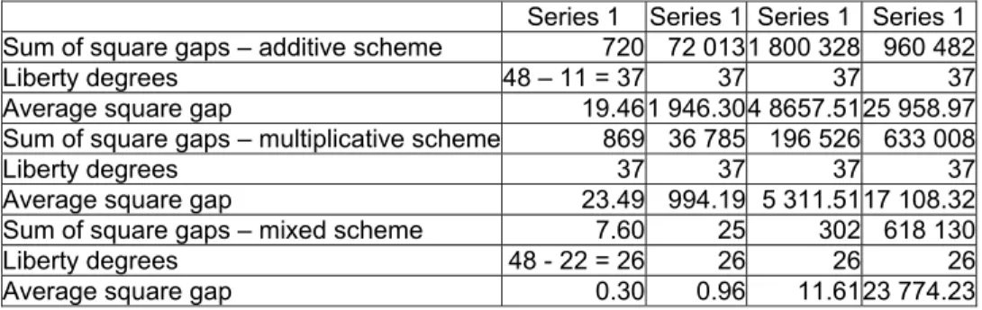
In order to evaluate each model’s performance, we choose the criterion which consists in comparing the average square gap (sum of square gaps divided by liberty degrees) between the theoretical observed values and the adjusted values with the help of each model (trend and type of seasonality), as according to Table 4.
Table 4 Sum of square gaps between the observed and the adjusted values
Series 1 Series 1 Series 1 Series 1 Sum of square gaps – additive scheme 720 72 0131 800 328 960 482
Liberty degrees 48 – 11 = 37 37 37 37
Average square gap 19.461 946.304 8657.51 25 958.97
Sum of square gaps – multiplicative scheme 869 36 785 196 526 633 008
Liberty degrees 37 37 37 37
Average square gap 23.49 994.19 5 311.51 17 108.32
Sum of square gaps – mixed scheme 7.60 25 302 618 130
Liberty degrees 48 - 22 = 26 26 26 26
Average square gap 0.30 0.96 11.61 23 774.23
One may note that estimating seasonal coefficients through the mixed method confers correct estimations and dominates very clearly the other two methods, except when the chronological series is affected by a non-linear trend (series 4).
Another approach will consist in eliminating seasonality first according to an additive scheme, and afterwards over a CVS series according to a multiplicative scheme. An attempt made on series 1 proved to be disastrous (sum of square gaps = 16 403 317) due to the creation of a new parasite cycle linked to the multiplicative seasonality.
7
. An example of application: The case of mobile
telephony
The mobile telephony market is a recent one, currently three operators acting on the French market: Orange, SFR, and Bouygues Telecom. This oligopolistic character generates a very powerful marketing activity, with very frequent new offers.
We are situated at the end of 1999 (a market not yet mature), a period for which forecasting the number of subscribers (the buying of Sim cards1) proved to be crucial
for each operator. The seasonality (Graph 1) indicates a very important peak in the months of December (gifts to individuals at the end of the year), because the number of subscribers is two times higher as compared to the average sales per year.
Two very distinctive segments of market in terms of behavior and seasonality are revealed, namely professional and private.
Graph 1 Number of subscribers (Sim cards sold) in the French mobile telephony,
in thousands
On this sales history (January 1995 to June 1999, 54 observations) we will apply the three methods of eliminating seasonality (Table 5), although the additive scheme, as we see on graph, turned out as proscribed.
1
The Correction of Chronologic Series’ Seasonal Fluctuations
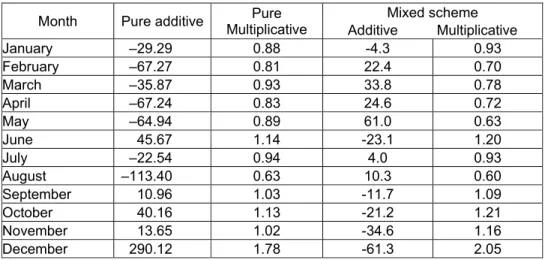
Table 5 Seasonal coefficients estimated as accordint to the three methods
Month Pure additive Multiplicative Pure Mixed scheme Additive Multiplicative January –29.29 0.88 -4.3 0.93 February –67.27 0.81 22.4 0.70 March –35.87 0.93 33.8 0.78 April –67.24 0.83 24.6 0.72 May –64.94 0.89 61.0 0.63 June 45.67 1.14 -23.1 1.20 July –22.54 0.94 4.0 0.93 August –113.40 0.63 10.3 0.60 September 10.96 1.03 -11.7 1.09 October 40.16 1.13 -21.2 1.21 November 13.65 1.02 -34.6 1.16 December 290.12 1.78 -61.3 2.05
Interpreting the estimated seasonal coefficients, one may note strong differences. It is interesting to observe that in the frame of the mixed scheme multiplicative and additive coefficients do not have the same profile of evolution. This suggests us that for the professional market, justifiable rather by the additive scheme which was already stabilized in 1998, the seasonal profile is not similar to the market for individuals, emphasized by the multiplicative scheme, with a market in full expansion referring to three moments: June (before leaving for holiday), October (opening of schools and universities) and December (Christmas and New Year’s holidays).
In order to evaluate the three methods’ relevance, we compare the square gaps sum (Table 6) of the observed values and adjusted values, with the help of a model with linear trend and seasonality.
Table 6 Square gaps sum of the observed and adjusted values
Additive scheme Multiplicative scheme Mixed scheme
Sum of square gaps 312 501 90 163 40 801
Liberty degrees 54 -11 = 43 43 32
Average square gap 7 267.46 2 096.81 1 316.16
Considering the standardization hypothesis of gaps, we will proceed to a Fisher test, such as: 10 , 2 51 , 3 32 / 40801 11 / ) 40801 90163 ( * = > 110,;0532 = − = F F .
This test permits predicting a significant difference of square gaps sum between the multiplicative and the mixed schemes.
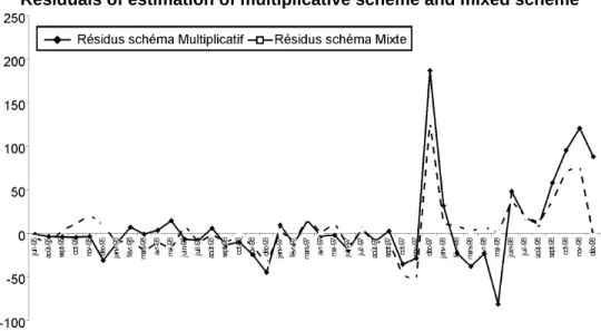
As we could anticipate, the additive scheme proves to be very weak; the mixed scheme turns out to be preferable to the pure multiplicative one (average square gap two times weaker). At last, we compare (Graph 2) the residuals of estimation between the mixed scheme and the multiplicative one.
Graph 2 Residuals of estimation of multiplicative scheme and mixed scheme
Over the period 1995-1998, the multiplicative scheme provides residual to estimation of equal amplitude with the residuals of the mixed scheme. In return, after 1998 –the period of emergence of the market of individuals – the mixed scheme offers an adjustment of better quality, as one may see in Table 7.
At last, one may note that in the case of using this method for developing forecasts, intervention variables for December 1997 and December 1998 should be integrated in the model.
Table 7 Sum of square gaps between observed values and adjusted values over
the period January 1998-June 1999
Multiplicative scheme Mixed scheme
Sum of square gaps 47 709 14 713
The mixed scheme, in this example and all over the period, seems preferable to a multiplicative scheme. Moreover, it allows for identifying, for this market, multiplicative
The Correction of Chronologic Series’ Seasonal Fluctuations
and additive seasonal coefficients corresponding to the two distinct markets (for professionals and for individuals), which emerged beginning with 1998.
8
. Concluding remarks
In this study, we have pointed out the issue of a probable existence of multiplicative and additive mixed seasonality. In this context, we presented through simulations that the elimination of seasonality following a pure additive scheme or a pure multiplicative scheme introduces a bias in the coefficients’ estimate and thus, consequently, in the calculus of the CVS series. The quality of demand analysis and, consequently, of sales forecasting will be affected by this.
Using a mixed technique of estimation allows for estimating simultaneously the trend coefficients and the additive and multiplicative seasonal coefficients functions perfectly if data series is affected by linear trend : we regain well the theoretical seasonal coefficients. A survey on the mobile telephony market indicates the superiority of the mixed method as compared to a multiplicative scheme and permits identifying the existence of a double seasonality : additive for enterprises and multiplicative for individuals. However, we think that the postulate of a linear trend is a limit of this method.
Thereby, a path for research consists in studying the robustness of seasonal coefficients’ estimators resulted from the mixed method function of the error of trend estimation.
R
eferences
Bourbonnais R., Terraza M., Analyse des séries temporelles, Dunod, 2004. Bourbonnais R., Usunier J–C., “Prévision des ventes”, Economica, 4 éd., 2007. Box G. E. P., Jenkins G. M., Time series analysis: forecasting and control,
Holden-day, 1976.
Dagum E. B., “Fondement des deux principaux types de méthodes de désaisonnalisation et de la méthode X11–ARMMI”, Economie
Appliquée, Vol 1, 1979.
Franses P., “Testing for seasonal unit root in monthly data”, Econometric Institute
Report, Erasmus University Rotterdam, 1990.
Hylleberg S., Engle R., Granger C., Yoo B., “Seasonal integration and co–integration”,
Journal of the Econometrics, 44, 1990.
Midgley and Dowling, “Innovativeness: The concept and measurement”, Journal of
Consumer Research, 4, 229-242, 1978.
Roehrich G., “Causes de l’achat d’un nouveau produit: variables individuelles ou caractéristiques perçues”, Revue Française de Marketing, No. 182, 2001
Shiskin J., “Electronic computers and business indicators”, National Bureau of
Annex Example of estimation of mixed seasonal coefficients for series x2,t
Analytic resolution series 2
DATA x2t Trend SMt ratio SAt ratio Forecast gap CVS
Year 1–J 257 510.6 0.70 –101.4 258.0 –1.05 509.14 F 192 520.6 0.60 –121.2 193.2 –1.17 518.66 M 809 530.6 1.30 117.4 809.1 –0.15 530.47 A 312 540.6 0.80 –121.6 312.8 –0.84 539.50 M 245 550.5 0.70 –141.4 246.0 –0.97 549.14 J 464 560.5 0.90 –41.8 464.6 –0.65 559.78 J 376 570.5 0.80 –81.6 376.8 –0.78 569.50 A 580 580.4 1.00 –2.0 580.4 –0.44 580.00 S 897 590.4 1.30 127.4 896.9 0.06 590.47 O 850 600.4 1.20 127.6 850.1 –0.06 600.34 N 893 610.4 1.30 97.4 892.9 0.13 610.47 D 988 620.3 1.40 117.2 987.7 0.34 620.58 Year 2–J 341 630.3 0.70 –101.4 341.8 –0.82 629.14 F 264 640.3 0.60 –121.2 265.0 –0.98 638.66 M 965 650.3 1.30 117.4 964.7 0.27 650.47 A 408 660.2 0.80 –121.6 408.6 –0.59 659.50 M 329 670.2 0.70 –141.4 329.7 –0.75 669.14 J 572 680.2 0.90 –41.8 572.4 –0.36 679.78 J 472 690.1 0.80 –81.6 472.5 –0.52 689.50 A 700 700.1 1.00 –2.0 700.1 –0.12 700.00 S 1053 710.1 1.30 127.4 1052.5 0.48 710.47 O 994 720.1 1.20 127.6 993.7 0.32 720.34 N 1049 730.0 1.30 97.4 1048.4 0.55 730.47 D 1156 740.0 1.40 117.2 1155.2 0.79 740.58 Year 3–J 425 750.0 0.70 –101.4 425.6 –0.59 749.14 F 336 760.0 0.60 –121.2 336.8 –0.78 758.66 M 1121 769.9 1.30 117.4 1120.3 0.69 770.47 A 504 779.9 0.80 –121.6 504.3 –0.33 779.50 M 413 789.9 0.70 –141.4 413.5 –0.52 789.14 J 680 799.9 0.90 –41.8 680.1 –0.07 799.78 J 568 809.8 0.80 –81.6 568.3 –0.26 809.50 A 820 819.8 1.00 –2.0 819.8 0.20 820.00 S 1209 829.8 1.30 127.4 1208.1 0.90 830.47 O 1138 839.7 1.20 127.6 1137.3 0.71 840.34 N 1205 849.7 1.30 97.4 1204.0 0.98 850.47 D 1324 859.7 1.40 117.2 1322.8 1.24 860.58 Year 4–J 509 869.7 509.4 –0.37 869.14 F 408 879.6 408.6 –0.59 878.66 M 1277 889.6 1275.9 1.12 890.47
The Correction of Chronologic Series’ Seasonal Fluctuations
DATA x2t Trend SMt ratio SAt ratio Forecast gap CVS
M 497 909.6 497.3 –0.29 909.14 J 788 919.5 787.8 0.23 919.78 J 664 929.5 664.0 0.00 929.50 A 940 939.5 939.5 0.53 940.00 S 1365 949.4 1363.7 1.33 950.47 O 1282 959.4 1280.9 1.10 960.34 N 1361 969.4 1359.6 1.40 970.47 D 1492 979.4 1490.3 1.70 980.58
prov.1 SM def.2 SM prov. SA def. SA
jan 0.70 0.70 –101.4 –99.4 feb 0.60 0.60 –121.2 –119.2 march 1.30 1.30 117.4 119.4 april 0.80 0.80 –121.6 –119.6 may 0.70 0.70 –141.4 –139.4 june 0.90 0.90 –41.8 –39.8 july 0.80 0.80 –81.6 –79.6 august 1.00 1.00 –2.0 0.0 sep 1.30 1.30 127.4 129.4 oct 1.20 1.20 127.6 129.6 nov 1.30 1.30 97.4 99.4 dec 1.40 1.40 117.2 119.2 12.03 12.00 –24.2 0.0 1
Prov = Provisional seasonal coefficients before standardization.
2