Ecological intuition versus Economic “reason”
Olivier Guéant, Roger Guesnerie, Jean-Michel Lasry
Ecological intuition versus Economic “reason”
y
.
Olivier Guéant
z, Roger Guesnerie
x, Jean-Michel Lasry
{July 10th 2011
Abstract
This article discusses the discount rate to be used in projects that aimed at preserving the environment. The model has two di¤erent goods, one is the usual consumption good whose production may increase exponentially, the other is an environmental good whose quality remains limited. The stylized world we describe is fully determined by four parameters re‡ecting basic preferences, "ecological" and intergenerational concerns and feasibility constraints.
We de…ne an ecological discount rate and examine its connections with the usual interest rate and the optimized growth rate. We discuss, in this simple world, di¤erent forms of the precautionary principle and show that cost-bene…t analysis should overweigh in a spectacular way the probabilities of the events associated with bad environmental outcomes..
Introduction
Environmentalists have often dismissed the economists’approach to environmental prob-lems, more especially when long term issues are at stake. On the one hand, what may be called "ecological intuition" puts high priority on the long run preservation of the environment. On the other hand, the cost-bene…t analysis promoted from economic rea-soning calls for the use of discount rates that apparently lead to dismissal of the long
We thank for useful comments on a previous version Ivar Ekeland, Vincent Fardeau, Thomas Piketty, Bertrand Villeneuve and Martin Weitzman. We also acknowledge useful exchange on this subject with Gary Becker, Steve Murphy and Joseph Stiglitz.
yThis work has been partly supported by Chaire Finance et Développement Durable.
zChaire Finance et Développement Durable, Université Paris-Dauphine, Place du Maréchal de Lattre
de Tassigny, 75116 Paris
run concerns. The climate issue is the most recent avatar of the clash between "eco-logical intuition" and "economic reason": in sharp contrast with most environmentalists and many climatologists’sensitivity, the computations based on Nordhaus (1993) suggest lenient climate policies. And although Nordhaus has been cautious in warning against mis-interpretations, some of his less cautious readers (Lomborg (2001)) claim that their …ght against climate policies proceeds from "economic reason". The Stern review (2006) has changed the tone of the debate signi…cantly. Although it is now gaining more acceptance, it is clear that Stern’s views of "economic reason" and of the subsequent cost-bene…t analysis may not be broadly accepted in the economic profession .
The present paper attempts to retackle the clear antagonism between the two sides from a simple model, that has been recurrently used in the economists’ debate, (see Krautkramer (1987), Heal (1998)). The relevance of the simple model in the present debate has been recently more systematically stressed by Guesnerie (2004), Hoel and Sterner (2007) and Sterner and Persson (2007). The model assumes that there are two goods at each period: the environment (a non-market good) and standard aggregate consumption. The …rst one is supposed to be available in …nite quantity when the second one is allowed to grow for ever. Indeed, modern optimism, based on the "economics" of past growth performance, leads to the belief that consumption of the so-called private goods may be multiplied without limit. In opposition, the "ecological" sensitivity stresses the bounded level of the environmental amenities : sites, lands, seashores, species are …nitely available on the planet.
We discuss the long run cost-bene…t analysis issues that arise within a model that has indeed two goods, with the respective interpretations of aggregate consumption and aggregate environmental quality that have just been introduced. As emphasized in Gues-nerie (2004), in such a setting, cost-bene…t analysis has to stress, not only the standard discount rates but also, the "ecological" discount rate, the evolution of which re‡ects the relative price of environment vis à vis the standard private good1.
The simple in…nite horizon world under scrutiny is entirely described by four parame-ters. The …rst parameter describes how substitutable are the standard and environmental goods in producing welfare. Opinions on the value of this parameter may di¤er between a "moderate" environmentalist and a "radical" environmentalist. The second parameter is the classical elasticity of marginal utility which re‡ects the extent to which welfare is subject to saturation, and which classically determines the intertemporal "resistance to substitution" (the inverse of the inter-temporal elasticity of substitution). The third
1It is well known that in an n-commodity world, there are as many discount rates as there are goods
parameter is a pure rate of time preference which, in this setting, measures the degree of intergenerational altruism of the agents. The last parameter will be an interest rate which, in the logic of a simple endogenous growth context (of the AK type), indicates to which extent one can transfer consumption between periods and generations.
Within this model, the research agenda is clear: we have to understand how the para-meters under consideration a¤ect the trade-o¤ between present and future consumption, both for standard or "environmental" consumption. As argued above, key dimensions of this trade-o¤ are captured through the "ecological" discount rates. Indeed, such rates provides central ingredients to the cost-bene…t analysis of actions, taken at the margin of the reference situation, aiming at preserving future environment. Our analysis then focus on the cost-bene…t analysis of actions aiming at avoiding "irreversible damage to the environment" : this brings us to assess the social value of what we call environmen-tal perpetuities, and to exhibit bounds that spectacularly illustrate the di¤ernce between such environmental perpetuities and standard …nancial perpetuities. This then leads us to examine and assess the logic of the precautionary principle which focuses attention on irreversible damage to the environment in case of "scienti…c uncertainty".
The paper proceeds as follows:
Part 1 of the paper presents the setting of the model and the role of the di¤erent parameters. We present the basic concepts and introduce the "ecological discount rate" independently of the growth model.
In Part 2, we introduce a two-good growth model à la Ramsey in which the environ-mental good quality remains constant over time. Along with the derivation of asymptotic results, the analysis allows us to exhibit the time pattern of both the optimal growth rates of private consumption and the "ecological discount rates". We are able to characterize yield curves in a way that allows us to single out a simple lower bound for the social loss due to an "irreversible damage to the environment" or, to put in another way to help us to price the so-called "environmental perpetuity".
Part 3 focuses on various forms of precautionary principles. We consider an irreversible damage to the environment that will take place at some later date and the e¤ect of which on (present and future) welfare is uncertain. We raise the question of the willingness to pay of the present generation in order to avoid such a damage. Indeed, the analysis in Part 2 provides an answer to the same question, when there is no uncertainty on the welfare e¤ect of the damage. When, as considered in this part, the damage has an uncertain impact on welfare, we stress …rst a "weak precautionary principle": it is reminiscent, for ecological discount rates, of Weitzman’s classical argument (2001) on long run standard discount rates. Second, we exhibit a "strong precautionary principle", which we view as
the most striking result of this paper. It tells us that the e¤ort of the present generation should be based on a cost-bene…t analysis which overweighs in a spectacular way the probabilities of the events associated with bad environmental outcomes.
The connections of the paper with the literature are as follows. Models with two-goods include Heal (1998)2. The model of the paper is the one considered in Guesnerie (2004),
and the argument exploits the …ndings of this paper. It also uses some of the insights of Hoel-Sterner (2007) and Persson-Sterner (2007), who have examined the same model and some further insights of Guéant-Lasry-Zerbib (2007). It also refers to the paper by Traeger (2010) who takes a broader perspective and improves on the previous results in a model allowing for environmental decay. All these papers refer to the concept of "ecological discount rates" emphasized in Guesnerie (2004) : this concept has also been stressed in a somewhat more complex setting than ours, and with a di¤erent focus, by Gollier (2009), . Note also that the importance of substitutability, which we emphasize here, has been stressed earlier in Neumayer (2002) and Gerlagh-Van der Zwann (2002).
Note that the views presented here on discounting and precaution have a motivation closely connected to the one of Weitzman (2009). However our emphasis is on relative prices e¤ects: even if we put emphasis on the uncertainty that surrounds the long run environmental issues and on the weight to be put on the bad case, we do not stress "fat tails".
1
Model and preliminary insights
1.1
Goods and Preferences
We are considering a world with two goods. Each of them has to be viewed as an ag-gregate. The …rst one is the standard aggregate private consumption of growth models. The second one is called the environmental good. Its "quantity" provides an aggregate measure of "environmental quality" at a given time. It may be viewed as an index re‡ect-ing biodiversity, the quality of landscapes, nature and recreational spaces, the quality of climate, the availability of water.
We call xt the quantity of private goods available at period t, and yt the level of
environmental quality at the same period. Generation t, that lives at period t only, has ordinal preferences, represented by a CES utility function: v(xt; yt) =
h x 1 t + y 1 t i 1
However, the measurement of cardinal utility, on which intertemporal judgements of
2There is also a related literature, which considers, as second good, an exhaustible resource. For recent
welfare will be made, involves an iso-elastic function: V (xt; yt) = 11 v(xt; yt)1
The above modeling calls for the following comments: Concerning v; we have to stress two points:
–The reader has noted that xt and yt appear with the same coe¢ cient in the
function v. However, for a given generation, this may be viewed as re‡ecting a choice of unit in the measurement of yt. Hence, giving the same weight to
the private good index and to the environmental quality index is a matter of notational convenience. However, leaving these weights constant across time or at least bounding them to be non vanishing, is a substantive assumption. It implies in particular that the concern for any of the two goods does not shrink. The present assumption on the symmetric role of x and y is intended to re‡ect the fact that we "only have one planet", the preservation of which is not, and will never be, a point of minor concern for its inhabitants, whatever their ability to produce large quantities of new private goods. Even, if the speci…c modeling is crude, this point seems well taken for our purpose in the sense that we do not deny a priori the soundness of "ecological intuition".
–v is a CES utility function, where is the elasticity of substitution between the two goods3. It describes a speci…c pattern of substitution: when the ratio environmental quantity (here quality) over private good quantity decreases by one per cent the marginal willingness to pay for the environmental good, or its implicit price, increases by 1= per cent.
This setting with constant elasticity of substitution allows to write easily what may be called the Green NDP. If we indeed regard the consumption good as the numéraire, then the number y x
y
1
is what we call Green NDP. Note that it grows inde…nitely whenever x grows inde…nitely, if, as we suppose here, y remains …nite. Note also that the ratio of Green NDP over standard NDP is (independently of any numéraire) = xy 1
1
and the ratio of green NDP to
total NDP is = 1+ .
Let us come to V . The marginal utility of a "util" of v, takes the form v : when v increases by one per cent, marginal cardinal utility decreases by per cent. This coe¢ cient 1 has the standard interpretation of an intertemporal elasticity of sub-stitution .
1.2
Social welfare
Social welfare is evaluated as the sum of generational utilities. In line with the argument of Koopmans, we adopt the standard utilitarian criterion:
1 1 +1 X t=0 e tv(xt; yt)1
Two comments can be made:
The coe¢ cient is a rate of pure time preference. Within the normative viewpoint which we mainly stress here, the fact that this coe¢ cient is positive has been crit-icized, for example by Ramsey who claims that this is "ethically indefensible and arises merely from the weakness of the imagination" or Harrod (1948) who views that as a "polite expression for rapacity and the conquest of reason by passion". Reconciling these feelings with Koopmans’ argument leads however to accept a positive and small . The smaller the , the more "ethical considerations become preponderant". Along the "ethical" line of argument, it has been argued that the number might be viewed as the probability of survival of the planet.
We may view the coe¢ cient as a purely descriptive one, re‡ecting intertemporal substitution and risk behavior, or as a partly normative coe¢ cient, re‡ecting the desirability of income redistribution across generations. This is the more frequent interpretation we stress in the paper: a low (resp. high) re‡ects little (resp. a lot of) concern for intergenerational equality.
At this stage, something more can be said on the philosophy of the approach taken here.
We have adopted a stylized description of the trade-o¤ between environmental quality and private consumption. We recognize that the modeling of the trade-o¤ is crude. How-ever if the degree of substitutability between standard consumption good and environment is …xed, we leave its value open. At this stage, we do not decide whether is smaller, a plausible short run hypothesis4, or greater than one, and we leave it …xed. We associate
a high , (resp. low ) to a moderate, (resp. radical) environmentalist’s viewpoint, the dividing line being obviously = 1.
At this stage, one should give some insights on the qualitative di¤erences between the cases > 1 and < 1, i.e. between the opinions we attribute respectively to the
4Since the marginal willingness for environmental amenities seems to grow faster than private wealth.
"moderate" and the "radical" environmentalists. These di¤erences echo the views that shape the understanding of the future long run usefulness of environmental quality when compared to private consumption.
First, let us consider > 1. We have v(xt; yt) = xt 1 + yxtt
1 1
and hence v grows as xt whenever xytt tends to zero. The asymptotic relative contribution of
environ-ment to welfare is vanishing and similarly, the Green NDP becomes small when compared to standard NDP. As we shall see later, the moderate environmentalist is very moderate in the long run.
On the contrary, in the case where < 1, it is useful to write v(xt; yt) = yt 1 + yxt
t
1 1
. In that case, v does not grow any longer inde…nitely with xt, but tends to y (if yt = y
for t 0). The increase in the consumption of private goods still contributes to welfare but with an asymptotic limit associated with the level of environmental quality. Standard NDP becomes small with respect to Green NDP.
Before turning to the intertemporal social optimum in a Ramsey growth model, we need to introduce the main concept of this paper, namely the ecological discount rate.
1.3
Ecological discount rate
1.3.1 De…nitions
In order to give some intuition on the question of discount rates, we shall consider a trajectory of the economy where environmental quality is …xed at the level y and where the sequence of private goods consumption denoted xt is also given (we will note gt the
growth rate implicitly de…ned by xt+1 = egtx
t).
We shall investigate the implicit discount factors at the margin of our reference tra-jectory, that is the discount rates that make the reference trajectory locally optimal. De…nition 1 The implicit discount rate for private good between periods t and t + 1, is rt such that
e rt = e @xV (xt+1; y)
The discount rate between periods 0 and T is then classically de…ned as : R(T ) = 1 T T 1 X t=0 rt
The discount rate R(T ) tells us, as is standard, that one unit of consumption at period T, is (socially) equivalent to e R(T )T today.
We then introduce the ecological discount rate, which as stressed in Guesnerie (2004), is the discount rate speci…c to the environmental good5.
De…nition 2 The ecological implicit discount rate between two consecutive periods is t de…ned by:
e t = e @yV (xt+1; y)
@yV (xt; y)
The discount rate between periods 0 and T is:
B(T ) = 1 T T 1 X t=0 t
The ecological discount rate tells us that one marginal improvement of environment at period T is socially equivalent to e B(T )T of the same improvement occurring today.
It implies that the present generation, when viewing an improvement of environment occurring at period T (the improvement being for example triggered by some present spending), should compare the present cost with the discounted value (discounted with the ecological discount rate) of the present marginal willingness to pay for the same improvement today. (This is what is called "standard" ecological cost-bene…t analysis by Guesnerie (2004)).
1.3.2 General properties
We now provide explicit formulas for the implicit discount rates along any given trajectory. Proposition 3 The implicit private discount rate for the private good between periods t and t + 1 can be equivalently written as either:
rt= + gt + 1 1 ln 1+ t
1+ t+1
or
5Hoel-Sterner (2006) consider the same model as here or as in Guesnerie (2004), without referring
rt= + gt= + 1 1 ln 1+ t 1 1+ t+1 1 where t = yt@yV xt@xV = xt yt 1 1
is the ratio of Green NDP over standard NDP.
The …rst formula shows how the standard logic of discount rates (rt = + gt ) is a¤ected by the environmental concern. The correction depends upon the evolution of the ratio t of Green NDP over standard NDP. The second formula looks strikingly di¤erent
from the …rst one, although it is equivalent, but it puts emphasis on factors that will turn out to be dominant when < 1.
Now, we can …nally relate the ecological discount rate to the interest rate:
Proposition 4 The ecological discount rate between periods t and t + 1 is related to the interest rate by:
t= rt gt=
This last formula stresses the e¤ect of the growth of private consumption on the ecological discount rate: it is qualitatively unsurprising that it is connected to the standard discount rate with a negative correction that increases with the growth rate and decreases when the elasticity of substitution increases. This formula, which captures the relative price e¤ect that we are stressing here is particularly simple and intuitively appealing. We can think about it as follows: it would be equivalent to give up one unit of environmental quality at the present period t, in order to provide e t of environmental quality tomorrow,
but the suggested move is equivalent, from the viewpoint of both generations, to give up !t units of private goods (where !tis the willingness to pay for environmental amenities)
and to provide !tert units, as soon as !tert compensate for one unit of environmental
quality at time t + 1, which is the case, if and only if !tert = !t+1e t:It is straightforward
that !t+1 = !tegt= so that !tert = !tegt= e t. The conclusion follows and stresses a key
ingredient for the understanding of the argument of the present paper6.
6If as in Traeger (2010), environmental quality were declining at rate g0; the formula becomes :
2
Optimized growth: private consumption,
ecologi-cal discount rates and their evolution
2.1
Introduction
In Guesnerie (2004), asymptotic results for the ecological discount rate were derived at the margin of any trajectory, whether the considered trajectory was non-optimal, or optimal either in a …rst best sense or in a second best sense. Here the evolution of ecological discount rates is going to be studied at the margin of an optimal trajectory that depends on the value of the parameters. There is indeed a priori no reason to refer to the same growth rate of consumption under di¤erent assumptions on , since these assumptions re‡ect di¤erent views (moderate or radical) of the contribution of the environment to welfare, and then potentially very di¤erent views on desirable growth.
In our model, we stick to the option of a …xed environmental quality, but put emphasis on the endogeneity of private consumption and we choose the simplistic endogenous set-ting of the AK type, where the interest rate r is exogenous, being then a one-dimensional su¢ cient statistics of the intertemporal production possibilities7. Hence, as announced in
the introduction, our discussion within the model will focus on four parameters only. A …rst one, , associated with the ecological concern, a second one, , linked to the intertem-poral structure of preferences, the third one, , associated with "ethical" considerations and the last one, r, describing economic constraints.
2.2
Optimized growth and asymptotic results
Our viewpoint is normative, and we refer to the intertemporal social welfare function introduced above. The "social Planner" maximizes:
1
X
t=0
e tV (xt; yt)
Our modeling choice leads the following economic and environmental constraints: Economic constraints: t+1 = er( t xt)where t stands for the wealth at date t 8.
Environmental constraints: The environmental quality is limited to y that is: yt y:
7Note that such an interest rate r can be extracted from a research arbitrage equation (as in
Aghion-Howitt (1998)), partly disconnected from the core model.
8A slightly more sophisticated version allows
t+1 = exp(r)[ t xt+ wt], where t stands for the
wealth at date t and wt is a possible exogenous production ‡ow that introduces no binding constraint
We naturally assume that r > : Furthermore, in this model, it is easy to check that optimization would lead to an in…nite postponement of consumption if r(1 ) > . We rule this out and assume that > 1-r. This means, given the order of magnitude that we have in mind for , that we will consider that is essentially greater than 1.
This hypothesis on the elasticity of intertemporal substitution goes with another one that is going to be made in the remaining of this paper, namely > 1. Because we suppose that > 1, this is simply a hypothesis on , which is supposed not to be too small9.
The next proposition gathers all the asymptotic results of social optimization. The …rst part stresses that optimality requires asymptotically constant growth whatever the parameters under scrutiny. However, both the asymptotic economic growth rates and the long run ecological discount rates crucially depends on the value of and :
Proposition 5 At the optimum, the private goods consumption grows asymptotically,
whatever ; .
The optimal asymptotic growth rate for the private good xt depends on and is given by the following formulae:
- If > 1 then g1 = r
- If < 1 then g1 = (r )
The asymptotic ecological discount rate, associated with the socially optimal trajectory is B1= limT !+1B (T ) given by the following formulae:
- If > 1 then B1 = 1 1 r + 1
- If < 1 then B1 = .
For > 1, the asymptotic growth rate of consumption is r , …tting the standard formula of the one-good model: the presence of the environmental good has asymptotically no in‡uence on the growth rate (although it does on the optimal trajectory). However, even in this case, the asymptotic ecological discount rate is always smaller than r.
The result for the other case ( < 1) may be surprising for two reasons: …rst, it was, a priori, unclear that the "radical" environmentalist would choose a positive asymptotic
9The di¤erences generated by the fact that > 1 or < 1 are emphasized in Traeger (2010). Our
choice on this subject has just been explained, and re‡ects our viewpoint, optimisation in an AK model, and our informal assesment of the "reasonable" values for the parameters. Note however that we expect the ‡avour of all our conclusions be kept or even reinforced in the case not considered here (decreasing or intuitvely increases the argument for a voluntarist environmental policy).
growth10. The second point is more surprising since the asymptotic ecological discount
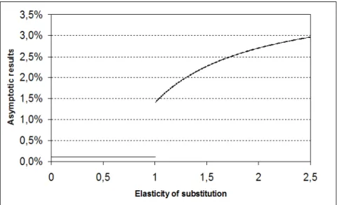
rate is totally disconnected from r and is very low since we assume to be close to zero. The opposition between the "radical" environmentalist and the "moderate" one is clearly stressed by the behavior of the ecological discount rate. The asymptotic di¤erence is again spectacular, as shown if we plot the asymptotic ecological interest rate as a function of :
Figure 1: Dependence on of the variable B1 when = 1:5; r = 4% and = 0:1%
10The evoked "intuition" is clearly not well grounded here since our model does not consider the
contribution of growth to environmental degradation. Introducing this phenomenon would indeed restore to some extent the validity of the intuition.
For instance, if one considers an exogenous exhaustion of the environment at rate g0, the asymptotic
ecological discount rate is B1given by g0 if < 1 and by (1 1 )r + 1 g0
if > 1: Hence, the e¤ect of the exhaustion is to decrease the ecological discount rate that can even be negative.
The asymptotic results stress a discontinuity in the world around = 1: However, the signi…cance of the discontinuity is clari…ed, and quali…ed, by the next result.
Proposition 6 At each period T, the optimal trajectory, is a continuous function of the parameters . Subsequently, 8T < 1; 7! B (T ; ) is continuous.
In a sense, the discontinuity associated with = 1 is worrying and might be viewed as an objection11 to our (admittedly crude) modeling choice. The above continuity result, which says that at any given period results are continuous functions of , weakens the objection: the discontinuity "in the limit" is compatible with continuity "at the limit": indeed B (T ) is a continuous function of when T is …xed (and …nite), as stated above.
All these results suggest to put the emphasis on the trajectory of discount rates.
2.3
The dynamics of ecological discount rates
Here, we are focusing attention on the evolution of ecological discount rates with time, and what can be called yield curves for ecological discount rates B (T ).
Since B (T ) = r 1 1T PTt=01gt, the dynamics of the ecological discount rate is linked to the dynamics of growth. Indeed, the dynamics of optimal growth can be assessed here (we still suppose that > 1).
Proposition 7 gt converges monotonically toward its limit according to the following rules:
- If < 1 then gt is increasing - If > 1 then gt is decreasing
Corollary 8 The shape of the yield curve is the following:
- If < 1 then T 7! B (T ) is decreasing (resp. increasing) and converges towards . - If > 1 then T 7! B (T ) is increasing (resp. decreasing) and converges towards
1 1 r + 1 .
To illustrate our proposition, we drew yield curves using a simulation of the growth path. Two examples are given below where the x-axis represents years and the y-axis the value of the ecological discount rate.
Yield curve example ( = 0:8, = 1:5, r = 4%, = 0:1%)
Yield curve example ( = 1:2, = 1:5, r = 4%, = 0:1%)
As it comes from the previous statements, in the …rst case ( < 1), the yield curve is decreasing and converges towards . In the second case ( > 1), the yield curve is
increasing and converges towards 1 1 r + 1 .
The …gures suggest that ecological discount rates converge slowly to their asymptotic value. Another interesting and related visual insight is that, when is low, the rate is low, but, even when is high, because the curve is increasing, the environmental rate is still
low in the medium run. Hence, what the …gures show is that, for a time period between 1 and 2 centuries from now, the disagreement between the radical environmentalist and the moderate environmentalist is not huge: the …rst one is between 0:45% and 0:35% and the second one is between 0:95% and 1:2%. Their willingness to pay, for say a generation living at date 150 equals the discounted value, with the ecological discount rate, respectively roughly 2=3 and 1=3, multiplied by their own marginal willingness to pay, which itself depends on their wealth and on their "ecological" views or intuition.
Note …nally that the knowledge of the ecological discout rates provides us all the information required for the cost bene…t analysis of actions aiming at improving (slightly) environmental quality at the margin of the optimized situation. The cost that one is willing to pay, at time 0, for improving the environmental quality at any further time is the discounted value, with the ecological discount rate, of the present willingness to pay for the same improvement to-day. Naturally, environmental policies involve more complex trade-o¤ (as shown next when considering irreversible damages to the environment), but the basic principle is the one just described.
2.4
Environmental perpetuity
Yield curves provide a key information about the dynamics of ecological discount rates. It should be noted that the conceptually important information conveyed in Proposition 5 on the limit behaviour of discount rates has no clear operational consequence for cost bene…t analysis (we do not know how long is the long run). On the contrary, the understanding of the path of convergence stressed in Corollary 8 has an evident bite on the conclusions of cost-bene…t analysis. In what follows, we are going to consider a simple problem that brings a necessary brick to the understanding of the (less simple) issues associated with the worldwide debate on the so-called precautionary principle.
The problem under scrutiny is the following: consider a damage to the environment that would take place today and say that, in order to avoid this damage for itself, the present generation is willing to pay x. How much should it be willing to pay if this damage not only occurs now but is irreversible, i.e. if it deteriorates the well-being of all future generations? Let us call mx the willingness to pay to avoid this damage for all future generations, instead of x; the willingness to pay when the damage is temporary12) and
only concerns the present generation.
In a sense, avoiding the damage can then be viewed as providing x environmental perpetuities, (a perpetuity being an in…nitely lived environmental service giving one unit
of environmental good at each period). Hence m is the "price" to be given to each of these perpetuities.
We provide here a lower bound on m.
Proposition 9 Let’s introduce a = r(1 1 ) + 1 .
In the present deterministic context, if the initial generation is willing to pay x in order to avoid a temporary (here one year) damage, it is willing to pay mx to avoid making it irreversible, where the number m is greater than 1a
The reader will notice that, in our admittedly simple world, the result has a striking simplicity and robustness. First, the lower bound to m, is valid both13 for > 1; and
for < 1. Second, it is also remarkable that the bound on m does not depend on initial wealth.
Let us note that if the planner neglected the relative price e¤ect associated with the increase in relative desirability of the environmental good, the discount rate would be r and m would be approximately 1r (approximately because we use an exponential discounting) as for a classical perpetuity. Hence, the introduction of the environmental good can drastically change the willingness to pay of the present generation for an environmental perpetuity that protects all future generations from an irreversible damage. For instance, if we consider that ' 0, then m is, in our deterministic study with > 1, greater than the "naive" assessment 1r, the multiplier being 1 11 . If we consider the parameters values
associated with the above graphs ( = 1:5), instead of having m ' 25 (resp. m ' 50) for
r = 4% (resp. r = 2%), we get when = 0:8; m 6 25 = 150 (resp. m 300) and
with = 1:2, m 2:25 25' 56 (resp. m 112:5)
Let us now consider the case where the irreversible damage will occur later in period , possibly far away from now. Again, the above question is meaningful, although m is no longer a priori necessarily greater than one.
Proposition 10 m > e a 1 a
The previous proposition told us that a may be viewed as an upper bound for the discount rate to be used for evaluating "environmental perpetuities". It is remarkable that the present proposition tells us that the same is true, i.e. a can consistently be used to provide a lower bound of the value of what might be called an "environmental forward perpetuity".
13However, the result depends on our hypothesis > 1. If < 1 then the lower bound is nothing
3
Precautionary principle: how to tackle the
uncer-tainty about the elasticity of substitution
?
3.1
An unusual form of uncertainty
3.1.1 Introduction
In the preceding part on environmental perpetuities, we focus on the desirable action to be taken in order to avoid an "irreversible damage to the environment". The so-called precautionary principle, in its most standard formulations, stresses the uncertainty surrounding a damage: "Where there are threats of serious or irreversible damage, lack of full scienti…c certainty shall not be used as a reason for postponing cost-e¤ective measures to prevent environmental degradation". This leaves somewhat open the question of the right intensity of action. This is the question tackled in this section. It suggests cost-bene…t analysis tools, aimed at evaluating the desirability of precaution in a situation where uncertainty plays a major role.
In the present framework, we focus attention on an irreversible damage, that will take place in the future, and whose harmfulness is now unclear but will be fully revealed when the damage occurs. Noteworthy, we do not consider that the damage itself has an uncertain intensity, although this is clearly the case in reality. Rather, our focus is on its harmfulness. In other words, we will focus on the uncertain impact of the damage in terms of welfare. Indeed, we believe that, as far as the environmental protection of the planet and climate change in particular are concerned, an important part of the uncertainty originates in the extent of the welfare impact of "ecological accidents" and not only on their intensity.
Formally, we assume that the uncertainty bears on the welfare function and more precisely on : in the …rst periods, this uncertainty is not resolved and can take two values: lor h( l< 1 < h) –and we attribute probabilities p and 1 p to the respective
cases. The two values re‡ect the a priori viewpoints of what we have called the radical and the moderate environmentalist. At time , an irreversible damage to the environment will take place (it consists here, of a small decrease of y) and the social cost of the damage will be revealed, i.e. the true value of will be known (either l or h). In a sense, the
occurrence of the environmental "accident" at time ; provides an experiment that allows to assess exactly the value of . The fact that nothing will be learnt between now and remains extreme. This assumption simpli…es the analysis, an analysis which remains an unavoidable reference and a prerequisite to the consideration of progressive accrual of the
3.1.2 The optimization problem
As suggested above, let us assume that 2 f l; hg, where l < 1 < h is learnt
instan-taneously at a time > 0. The new optimization problem to determine the consumption path is the following:
1
X
t=0
e t[pV ( l; xt; y) + (1 p)V ( h; xt; y)] + pU( ; l) + (1 p)U( ; h)
with 0 given, t+1 = er[ t xt] and where U( ; ) = Max(xt)t
P1
t= e
tV ( ; x t; y) is
the Bellman function associated with the non-random problem after we learnt . At this time, the deterministic results provide the required information, given the initial condition which is the remaining wealth .
The next paragraphs stress that the case < 1should be weighted signi…cantly in our present decisions, even if it is unlikely. We will present di¤erent forms of this result that clearly echo the just discussed precautionary principle.
3.1.3 A …rst result: a weak precautionary Principle
The …rst version of this precautionary principle (the weak precautionary principle) is an asymptotic statement: the rate to be used to discount environmental good is asymptoti-cally the ecological discount rate corresponding to the smallest (i.e. = l < 1). The
second and stronger form of precautionary principle bears on the way m depends on p. The resolution of the above problem is similar to what we have done before in the deterministic case, at least for the asymptotics. After has been elicited, the two trajec-tories x l
t and xth which are identical for t < , diverge: if is equal to l the asymptotic
growth rate of xt = x l
t is g1 = l(r ) and if is equal to h the asymptotic growth
rate of xt = x h
t is g1= r .
Using these asymptotic results on growth and the formula de…ning the ecological discount rate in this context – namely e B (T )T = e T hp@yV ( l;xTl;y)+(1 p)@yV ( h;xTh;y)
p@yV ( l;x0;y)+(1 p)@yV ( h;x0;y)
i – we can deduce the asymptotic value of the ecological discount rate.
Proposition 11 (Weak Precautionary Principle).Viewed from time zero the
asymp-totic ecological discount rate B1 does not depend on p > 0 and is equal to
B1=
Uncertainty leads to consider asymptotically the smallest possible ecological rate. This is the counterpart for the "ecological discount rate" of the limit behavior of discount
rates, stressed by Weitzman (2001). This is a precautionary principle, in the sense that it suggests to put emphasis on the long run bad situations even if uncertain. It is weak, since, as argued above, its operational content for cost-bene…t analysis is almost nil. The next paragraph provides an operational precautionary principle.
3.2
Strong precautionary Principle
3.2.1 The question
The question raised in this Section is similar to that raised in a deterministic context: how much is the present generation willing to pay in order to avoid an irreversible damage
to the environment, that would take place at time ? However, and contrary to our
deterministic case, the harmfulness of the (…xed) damage in terms of welfare is not well ascertained.
Our objective is to generalize the previous deterministic results on the multiplier m, which relates the willingness to pay of the present generation14 to avoid the damage for itself, forgetting about its descendants or viewed as temporary, to its willingness to pay to avoid the irreversible damage at date :
We know the answer in the limit deterministic cases: m has a lower bound e a 1
a where
a = a(l) = r(1 1
l ) +
1
l if is equal to l, and similarly a = a(h) = r(1
1
h ) +
1
h
if is equal to h.
What are plausible conjectures on the bounds on the multiplier in the stochastic
case? One may expect m to be bounded from below by an expression of the form
e a hp 1
a(l) + (1 p) 1 a(h)
i
, where a would neither be a(h) nor a(l) and where the term between bracket is the expected value of the future damage to the environment as seen from period :
The following proposition shows that the intuitive conjecture is valid only once the probability of the bad case15 is biased upward. Indeed, this upward bias is spectacular:
Proposition 12 (Strong Precautionary Principle, …rst version)
Let’s introduce, as in the deterministic case, a(h) = r(1 1
h ) + 1 h and similarly a(l) = r(1 1 l ) + 1 l .
14Note, that naturally, the willingness to pay of the present generation depends on its wealth and on
the true value of . In the uncertain case under scrutiny, again the willingness to pay of the present generation does depend on the plausibility of the two cases, as measured by p, the probability of being characterized by a low .
15The bad case here, and from now, refers to the case of a low ( =
In the random case, if p lies in (0; 1), we have: m > e B ( ) 1 a(l) pN ( ) pN ( ) + (1 p) + 1 a(h) (1 p) pN ( ) + (1 p)
where N ( ) > 1 grows exponentially with .
The above formula provides information on the bounds on m that, as desirable, do encompass the information obtained in the deterministic case. Note however, that the bound we …nd here does not only depend, as in the deterministic case, on the four ba-sic parameters of the models, but also on the characteristics of the initial situation (in particular through N ( )).
The proof is given in the appendix, but we may give some insights into it. The fact that we discount at time 0 the willingness to pay at with the ecological discount rate B ( ) is intuitively unsurprising, as well as the consequence of easy algebra. As suggested above, the fact that the (bounds on the) value of the irreversible damage to the environment, seen from period , when the bad case occurs (resp. the good case), be proportional to a(l)1 (resp. a(h)1 ) is, in view of our previous results, intuitive. Now, concerning the weights to associate to each case, it may be less intuitive that the ratio of the appropriate corrections to be made to p and 1 p has to be the ratio of the marginal utility of the environment in the bad and in the good cases, which is nothing else that N ( ): The fact that N ( ) increases with , and is unbounded, follows from the examination of the formulas, just in line with the intuition brie‡y presented in Section 1.
Hence, the expectation of the deterministic lower bounds stressed in Proposition 9, (which comes naturally into the picture, as suggested above) has to be measured with distorted probabilities. Indeed, the probability to attribute to the bad case with respect to the good case has to be severely distorted: the later the date, the more weight we put on the bad case, the weight becoming closer to its limit 1, counteracting the (weak) tendency of the (ecological) discount rate to dismiss precaution for late damages. Let us be more explicit on that by considering the following corollary:
Corollary 13 (Strong Precautionary Principle, second version). There exists a
function (p; ) 7! (p; ), concave with respect to p, verifying:
(0; ) = 1 a(h) (1; ) = 1 a(l) d dp(p = 0; ) = 1 a(l) 1 a(h) N ( ) !+1!+1
d dp(p = 1; ) = 1 a(l) 1 a(h) 1 N ( ) !+1!0 lim !+1 (p; ) = 1 a(l);8p > 0 such that: m > e B ( ) (p; )
To well understand the last statements, let us come back to the "plausible" conjec-ture discussed at the beginning of the subsection. It was suggested that m might be the discounted value (with the appropriate discount rate) of pa(l)1 + (1 p)a(h)1 : What our analysis says is that if is large, and p large, the intuitive formula tends to be right; but that when p is small, the lower bound on the multiplier is far from the discounted value of pa(l)1 + (1 p)a(h)1 and closer to the discounted value of a(l)1 . This is a clear and strong form of precautionary principle. If we do not know whether or not an environmental accident will lead to real downfall in welfare in the future, here at date 100, a key element of our computation is, in a sense, to proceed as if the bad case were to happen for sure.
Let us illustrate the importance of the point with numbers. Suppose that we are in a world in which the present willingness to pay to avoid the irreversible damage from the viewpoint of the sole present generation welfare is let us say, 0:1% of its NDP, if the harm is minor in terms of welfare, and 1% if the welfare harm is high. What bounds can we …nd on its willingness to pay for avoiding the irreversible accident occurring at period = 100?
With the data previously used (r = 4%; = 0:1%; = 1:5; l = 0:8; h = 1:2), we have
a(l) = 1=150 and a(h) ' 1=56, so that e a(l) ' 1=2 and e a(h) ' 1=5:9. Hence, for a small p, say p = 1=10, the intuitive lower bound for the multiplier, applying broad linear approximations; is just below 14 (which means a willingness to pay to avoid the accident of 2:6% of NDP16). Now, with the bounds given in Proposition 12, the same calculations,
assuming is large enough to apply the approximation, give a lower bound for m equal to 31:5, i.e. a willingness to pay of around 6% of NDP (more than twice more), and this for a low probability of the occurrence of the accident... For a high probability accident, the lower bound on the multiplier is 75.
Although they are already large, we leave to the reader to view this numbers as applying metaphorically to the question of climate change, particularly in view of the fact that the computed multipliers are even far higher.
Indeed, although an exact solution of the optimization program is untractable ana-lytically, the random case can easily be solved numerically for all p’s. We illustrate our
results with the preceding set of parameters in which, as above, before time = 100 ( is revealed at this time), the agent hesitates between h = 1:2 and l= 0:8 (with
probabil-ities 1 p and p). In this situation, with r = 4%; = 0:1%; = 1:5 we …nd numerically the ecological discount rates and compute m for any possible p in [0; 1]:
This …gure illustrates in a spectacular way our qualitative statement: the function p 7! m(p) is quickly increasing (and concave). Hence, even for small p strictly greater than 0, m is far from m(p = 0) and closer to m(p = 1).
Conclusion
The paper proposes a simple model for discussing the long run issues associated with en-vironmental quality. The model describes a world with four parameters, that respectively re‡ect ecological concern, resistance to intertemporal substitution, intergenerational al-truism and feasibility constraints. These parameters are supposed to remain constant over time, an assumption which makes the model tractable and simple, although it is certainly too extreme. Note that the paper takes a parsimonious defence of the environmentalist viewpoint in the sense that we rule out values of parameters too much favorable to his views: we assume that growth has no negative e¤ect on the environment, etc.
The paper shows that long run environmental policies are crucially a¤ected by the "ecological view", in particular but not only, if the radical viewpoint is adopted. Also, the paper shows that the radical viewpoint on environment, even when it is unlikely to be true, has however bite on the determination of present policies, a fact that may be viewed as supporting some form of a precautionary principle. In a companion paper, (work in progress) we will provide back of the envelope computations based on an variant of the present model to the global warming issue that suggest an upward re-evaluation of the Stern estimates of the merits of action.
Let us repeat that our simple setting allows to focus both on the relative price e¤ect and on the uncertainty dimension of the economic appraisal of ecological intuition. To put it in a nutshell, the paper stresses that the "economic" argument, along which we should not sacri…ce the present generations’welfare to the welfare of our descendants that will be wealthier than us, is valid here, but has to be strongly quali…ed. There is a most valuable gift that is worth transmitting to our descendants, because it may be very important for them, although this is not sure. That gift is a good environment.
References
[1] P. Aghion, P. Howitt, M. Brant-Collett, and C. García-Peñalosa. Endogenous growth theory. the MIT Press, 1998.
[2] KJ Arrow, HB Chenery, BS Minhas, and RM Solow. Capital-labor substitution and economic e¢ ciency. The Review of Economics and Statistics, 43(3):225–250, 1961. [3] R.J. Barro and X. Sala-i Martin. Economic growth. MIT Press Books, 1, 2003. [4] P. Dasgupta. Human well-being and the natural environment. Oxford University
Press, USA, 2004.
[5] K. d’Autume, A.and Schubert. Hartwick’s rule and maximin paths when the ex-haustible resource has an amenity value . Journal of Environmental Economics and Management, 56(3):260–274, 2008.
[6] R. Gerlagh and BCC Van der Zwaan. Long-term substitutability between environ-mental and man-made goods. Journal of Environenviron-mental Economics and Manage-ment, 44(2):329–345, 2002.
[8] C. Gollier, B. Jullien, and N. Treich. Scienti…c progress and irreversibility: an eco-nomic interpretation of the “Precautionary Principle”. Journal of Public Ecoeco-nomics, 75(2):229–253, 2000.
[9] O. Guéant, J.M. Lasry, and D. Zerbib. Autour des taux d’intérêt écologiques. Cahiers de la Chaire Finance et Développement Durable,(3), 2007.
[10] R. Guesnerie. Calcul économique et développement durable. Revue économique, 55(2004/3):363–382, 2004.
[11] R. Guesnerie and H. Tulkens. The design of climate policies, 2008.
[12] R. Guesnerie and M. Woodford. Endogenous ‡uctuations. In Advances in Economic Theory: Sixth World Congress, volume 2, pages 289–412. Cambridge Univ Pr, 1992. [13] G. Heal. Valuing the future: economic theory and sustainability. Columbia Univ Pr,
2000.
[14] G. Heal. Intertemporal welfare economics and the environment. Handbook of En-vironmental Economics: Economywide and international enEn-vironmental issues, page 1105, 2003.
[15] C. Henry. Growth, intergenerational equity and the use of natural resources. Cahier du Laboratoire d’Econométrie, 529, 2000.
[16] M. Hoel and T. Sterner. Discounting and relative prices. Climatic Change, 84(3):265– 280, 2007.
[17] J.V. Krutilla and C.J. Cicchetti. Evaluating Bene…ts of Environmental Resources with Special Application to the Hells Canyon. Nat. Resources J., 12:1, 1972.
[18] F. Lecocq and J.C. Hourcade. « Incertitude, irréversibilités et actualisation dans les calculs économiques sur l’e¤et de serre» . Kyoto et l’Economie de l’e¤et de serre, rapport du CAE, pages 177–197, 2001.
[19] B. Lomborg. The skeptical environmentalist: measuring the real state of the world. Cambridge Univ Pr, 2001.
[20] JC Milleron, R. Guesnerie, and M. Crémieux. Calcul économique et décisions
publiques. La Documentation Française, 1978.
[21] W. Nordhaus and J. Boyer. Roll the Dice Again: Economic Modeling of Climate Change, 2000.
[22] W.D. Nordhaus. Rolling the’DICE’: An Optimal Transition Path for Controlling Greenhouse Gases’. Resource and Energy Economics, 15(1):27–50, 1993.
[23] N. Stern. The economics of climate change. American Economic Review, 98(2):1–37, 2008.
[24] N. Stern, S. Peters, V. Bakhshi, A. Bowen, C. Cameron, S. Catovsky, and D. Crane. Stern Review: The economics of climate change. 2006.
[25] T. Sterner and U.M. Persson. An even Sterner review: introducing relative prices into the discounting debate. Review of Environmental Economics and Policy, 2008. [26] C.P. Traeger. Sustainability, limited substitutability, and non-constant social
dis-count rates. Journal of Environmental Economics and Management, 2011.
[27] M.L. Weitzman. Gamma discounting. The American Economic Review, 91(1):260– 271, 2001.
[28] M.L. Weitzman. A review of the Stern Review on the economics of climate change. Journal of Economic Literature, 45(3):703–724, 2007.
[29] M.L. Weitzman. On modeling and interpreting the economics of catastrophic climate change. The Review of Economics and Statistics, 91(1):1–19, 2009.
4
Appendix
Proof of Proposition 3:
The implicit discount rate rtfor private goods between periods t and t + 1 is uniquely de…ned by:
e rt= e @xV (xt+1; y) @xV (xt; y) = e xt+1 xt 10 @xt+1 1 + y 1 xt 1+ y 1 1 A 1 1
Taking logarithms, this gives:
rt= + gt= 1 1 ln 0 @xt+1 1 + y 1 xt 1 + y 1 1 A = + gt= +1 1 ln 1 + t1 1 + t+11 !
This is the second formula of Proposition 3. The …rst formula can be obtained by the same reasoning:
rt= + gt= 1 1 ln 2 6 6 4 xt+1 xt 1 1 + y xt+1 1 1 + xy t 1 3 7 7 5 = + gt + 1 1 ln 1 + t 1 + t+1 ! Proof of Proposition 4: We have e t= e (@yV )t+1 (@yV )t = e (@xV )t+1 (@xV )t xt+1 xt 1= = e rtegt= and hence, t= rt gt= . Proof of Proposition 5:
We consider the Lagrangian of the problem L =P1t=0exp( t)[V (xt; yt) + t(er[ t xt] t+1) + t(y yt)]:
The …rst order conditions are the following: 8 > < > : @xtL = 0 () @xV (xt; yt) = er t @ t+1L = 0 () t+1exp(r ) = t @ytL = 0 () @yV (xt; yt) = t
The …rst thing to note is that yt = y. Then, since r > , tand @xV (xt; y)are both decreasing and tend to zero. The
natural consequence is that the consumption of the private good xt grows and tends to +1.
The growth path xt is then characterized by: xt
1h xt 1 + y 1i 1 1 = @xV (xt; y) = er t= 0e r exp((r )t) In the > 1 case, xt 1 0e r
exp((r )t). Hence, the asymptotic growth rate is the same as if there were no
consideration of the environmental good g1=r In the < 1case, xt 1 1 0er
y1 exp((r )t)
. Hence, the growth rate in that case is given by g1= (r ) The results on the ecological discount rate then follow from Proposition 4.
Proof of Proposition 6: (This proof can be omitted at …rst reading)
It’s very important here to consider v(x; y) = h12x 1 +21y 1i 1 with the weights 12 to extend the function properly and also to remind that V =v1 0 1
1 0 . Obviously, it doesn’t change anything to our preceding results since these
changes only consist in additive or multiplicative scalar adjustment. We have t= r
gt
and thus B (T ) = r 1 1Tln xT
x0 :
Therefore, the only thing to prove is that 8t; xt is a continuous function of . But we know that the growth path is
de…ned by the …rst order condition @xV (xt; ) = 0 er
exp((r )t) where we omitted the reference to y here since we focus on .
the Lagrange multiplier 0 is a continuous function of .
the function h( ; ) implicitly de…ned by @xV (g( ; ); ) = is continuous.
The second point is easy. Notice …rst that the function (x; ) 7! V (x; ) can be extended to a C2function (the proof
is easy). Then, by the implicit function theorem, h( ; ) is a C1function (( ; ) 2 R+ 2).
Therefore, the only thing to prove is that the …rst Lagrange multiplier 0 is a continuous function of . Let us recall that 0is de…ned by the resources constraintP1t=0xte rt=
P1
t=0h( 0erexp(( r)t); )e rt= 0+P1t=0wte rt(:= 11 7)
Here, we cannot apply directly the implicit function theorem to the left hand side. However, if we consider the restricted optimization problem with a …xed time horizon T1 8 then the associated Lagrange multiplier ( T
0) is implicitly de…ned by T X t=0 h( T0 exp(( r)t); )e rt= 0+ T X t=0 wte rt(:= T)
and the implicit function theorem applies: T
0 is a C1 function of .
Now, we can approximate 0by T0 and this gives: j 0( ) 0(~)j j 0( ) T0( )j+j T0( ) T0(~)j+j T0(~) 0(~)j.
Hence, we see that the only thing to prove is a pointwise convergence in the sense that, for …xed, we have a convergence of T0( )towards 0( )as T ! 1. To prove that let’s introduce FT: z 7!PTt=0h(zerexp(( r)t); )e rtand similarly
F : z 7!P1t=0h(zerexp(( r)t); )e rt. These two functions are positive and decreasing because h is a positive and
decreasing function of . Moreover, FT is continuous and there is a pointwise convergence of FT towards F . By monotony,
FT converges towards F uniformly on every compact set and therefore, F is a continuous function and so is the inverse of
the function F .
By the second Dini’s theorem then, the inverse of the function FT converges uniformly on every compact set towards the
inverse of the function F .
But T0 0= FT1( T) F 1( 1)and hence, since T! 1, we are done with the proof.
Proof of Proposition 7:
Let us go back the …rst order conditions that de…ne the growth path. We have @xV (xt; y) = er @xV (xtegt; y):
Therefore, the growth rate g, as a function of x is de…ned implicitly by (we now omit the y terms) V0(x) exp(r ) =V0 xeg(x) :
Taking logs and deriving we get VV000(x)(x)=
V00(xeg(x))
V0(xeg(x))eg(x)(1 + g0(x)x)
Hence, the sign of g0(x)is the sign of V0(x)V00(xeg(x))eg(x) V0(xeg(x))V00(x). This sign is simply the sign of d dx
V0(xeg) V0(x)
where g is now an independent variable. The latter expression can be written as e g= d dx y+(xeg) 1 y+x 1 1 1 : The sign of this derivative is the sign of 1 1 1 eg 1 1 = 1 eg 1 1
Since g > 0 in our context, this expression has the same sign as 1 and this proves our result. Proof of Proposition 9:
By de…nition, m is equal toP1T =0exp( B (T )T ).
Since we want to …nd a lower bound for m, we need to …nd an upper bound for B (T ). The ecological rate B (T ) can be written B (T ) = r 1
T
PT 1
t=0 gt:Hence, the problem boils down to …nd a lower bound
for gt.
Now, from Proposition 3, we know that a lower bound to gt is r so that B (T ) a. This gives m =P1T =0exp( B (T )T ) P1T =0exp( aT ) =1 exp(1 a) 1a:
Proof of Proposition 10:
17This quantity is supposed …nite for the problem to have a solution. 18M axPT
By de…nition, m is now equal toP1T = exp( B (T )T ):
Using the same inequality as before, we have m P1T = exp( aT ) = 1exp(exp(a )a) e a 1 a
Proof of Proposition 11:
Let’s consider T > and let’s recall …rst the de…nition of B (T ) in this context: B (T ) = 1 T ln " p@yV ( l; xTl; y) + (1 p)@yV ( h; xTh; y) p@yV ( l; x0l; y) + (1 p)@yV ( h; x0h; y) #
To prove our result, it is su¢ cient to prove that the expression in the logarithm remains bounded as T increases. Hence, we are going to prove that the following expression is bounded:
py 1 l x l T l 1 l + y l 1 l 1 l l 1 + (1 p)y 1 h x h T h 1 h + y h 1 h 1 h h 1
The …rst part of the expression converges toward py and is therefore bounded. For the second part of the expression, x h
T
h 1 h + y h
1
h ! 1 so that, since1 h
h 1 < 0(we supposed h > 1), the second
part of the expression tends toward 0 and this proves the result. Proof of Proposition 12:
For T , we have, by de…nition exp ( B (T )T ) = exp ( T ) p@yV ( l;xTl;y)+(1 p)@yV ( h;xTh;y)
p@yV ( l;x0;y)+(1 p)@yV ( h;x0;y)
We are going to separate the reasoning into two parts to factorize what happens after time on the two di¤erent trajectories. We have: exp ( B (T )T ) =pe (T ) " @yV ( l; xTl; y) @yV ( l; xl; y) # e @yV ( l; x l; y) p@yV ( l; x0; y) + (1 p)@yV ( h; x0; y) +(1 p)e (T ) " @yV ( h; xTh; y) @yV ( h; xh; y) # e @yV ( h; x h; y) p@yV ( l; x0; y) + (1 p)@yV ( h; x0; y)
The terms e (T ) @yV ( l;xTl;y)
@yV ( l;x l;y) and e
(T ) (1 p)@yV ( h;xTh;y)
@yV ( h;x h;y) can easily be controlled using what we know
from the deterministic cases: they are respectively greater than e a(l)(T ) and e a(h)(T ).
The other terms correspond to what happens before time and we would like to link them to the ecological discount rate B ( ).
Let’s take …rst the term corresponding to the "l-trajectory": e @yV ( l; x l; y) p@yV ( l; x0; y) + (1 p)@yV ( h; x0; y) = e p@yV ( l; x l; y) + (1 p)@ yV ( h; x h; y) p@yV ( l; x0; y) + (1 p)@yV ( h; x0; y) @yV ( l; x l; y) p@yV ( l; x l; y) + (1 p)@yV ( h; xh; y) = e B ( ) @yV ( l; x l; y) p@yV ( l; xl; y) + (1 p)@yV ( h; xh; y) = e B ( ) @yV ( l;x l;y) @yV ( h;x h;y) p@yV ( l;x l;y) @yV ( h;x h;y)+ (1 p)
Now, let’s turn to the term corresponding to the "h-trajectory": e @yV ( h; x h; y) p@yV ( l; x0; y) + (1 p)@yV ( h; x0; y) = @yV ( h; x h; y) p@yV ( l; xl; y) + (1 p)@yV ( h; x h; y) e p@yV ( l; x l; y) + (1 p)@ yV ( h; xh; y) p@yV ( l; x0; y) + (1 p)@yV ( h; x0; y)
= @yV ( h; x h; y) p@yV ( l; x l; y) + (1 p)@yV ( h; xh; y) e B ( ) = e B ( ) 1 p@yV ( l;x l;y) @yV ( h;x h;y)+ (1 p)
Now, if we compile all the inequalities, we obtain: e B (T )T > e B ( ) pe a(l)(T ) N ( )
pN ( ) + (1 p) + (1 p)e
a(h)(T ) 1
pN ( ) + (1 p) where N ( ) stands for @yV ( l;x l;y)
@yV ( h;x h;y)
If we sum everything, we get: m > e B ( ) p 1 a(l) N ( ) pN ( ) + (1 p) + (1 p) 1 a(h) 1 pN ( ) + (1 p) We see that one thing remains to be done: studying N ( ).
We can write: N ( ) = @yV ( l; x l; y) @yV ( h; xh; y) = 2 4y 1l x l l 1 l + y l 1 l 1 l l 1 3 5 = 2 4y 1h x h h 1 h + y h 1 h 1 h h 1 3 5 = 2 6 6 4y 2 41 + x l y l 1 l 3 5 1 l l 1 3 7 7 5 = 2 6 6 4y 2 41 + x h y h 1 h 3 5 1 h h 1 3 7 7 5 = 2 41 + x l y l 1 l 3 5 1 l l 1 = 2 41 + x h y h 1 h 3 5 1 h h 1
It’s clear that this expression grows exponentially with (since h > 1).
Also, under our hypotheses, this expression is always greater than 1 because we divide a term greater than 1 by a term smaller than 1.
Proof of Corollary 13:
From Proposition 12, we see that the only thing to prove is that the function
p 7! p 1 a(l) N ( ) pN ( ) + (1 p) + (1 p) 1 a(h) 1 pN ( ) + (1 p) lies above it chordh p = 0; 1
a(h) ; p = 1; 1 a(l)
i .