HAL Id: pastel-00002995
https://pastel.archives-ouvertes.fr/pastel-00002995
Submitted on 19 Dec 2007HAL is a multi-disciplinary open access archive for the deposit and dissemination of sci-entific research documents, whether they are pub-lished or not. The documents may come from teaching and research institutions in France or abroad, or from public or private research centers.
L’archive ouverte pluridisciplinaire HAL, est destinée au dépôt et à la diffusion de documents scientifiques de niveau recherche, publiés ou non, émanant des établissements d’enseignement et de recherche français ou étrangers, des laboratoires publics ou privés.
models, contributions and applications
Charles-Henri Florin
To cite this version:
Charles-Henri Florin. Spatio-temporal segmentation with probabilistic sparse models, contributions and applications. Mathematics [math]. Ecole des Ponts ParisTech, 2007. English. �pastel-00002995�
& %
Th`ese
Pr´esent´ee devant l’Ecole Nationale des Ponts et Chauss´ees en vue de l’obtention du grade de Docteur
par
Charles Henri Florin
Spatio-temporal segmentation with probabilistic sparse models, contributions and applications
soutenue le 4 Mai 2007
Pr´esident du jury Alain Rahmouni CHU Henri Mondor - Paris XII
Rapporteurs Allen Tannenbaum Georgia Tech
Jean-Philippe Thiran EPFL
Examinateurs Nicholas Ayache INRIA
Gilles Fleury Sup´elec
Renaud Keriven CERTIS, ENPC
Membre invit´e Gareth Funka-Lea Siemens Corp. Research Directeurs de th`ese Nikos Paragios Ecole Centrale de Paris
James Williams Siemens Medical Solutions
Ecole Nationale des Ponts et Chauss´ees,
77455 Marne la Vallee, France,
The intellectual property included in this thesis is protected by the following Siemens patent applications: 11/265,586 1164/KOL/05 11/303,564 11/374,794 11/384,894 PCT/US06/10701 11/511,527 60/812,373 60/835,528 60/889,560
Preface
This PhD was co-directed by Nikos Paragios from Ecole Nationale des Ponts et
Chauss´ees, then Ecole Centrale de Paris, and James Williams from Siemens
Cor-porate Research. I would like to warmly thank both my advisers for their time and
guidance on both sides of the ocean. Their academic and industrial experience
have brought me a wide perspective in the domain of Computer Vision. Nikos
Paragios has successfully guided my research remotely from France and James
Williams has always offered me the necessary time to share his experience with
me.
Renaud K´eriven, director of CERTIS lab at Ecole Nationale des Ponts et Chauss´ees
welcomed me at the very beginning of the PhD, where I had the opportunity to
meet with talented researchers and benefit from their experience; for that, I am
thankful to the CERTIS lab and in particular to Renaud.
Romain Moreau-Gobard guided my first steps at Siemens Corporate Research
and supported my first research projects. The exceptional conditions for research
created by the people at SCR has had a great impact on my work. I would like
to thank in particular Marie-Pierre Jolly for her support; she has brought me both
efficient research organization skills and personal support. Mika¨el Rousson and
Christophe Chefd’hotel for their kind support and friendship, and all the people at
SCR with whom I had fruitful and challenging scientific discussions.
Last but not least, I am specially grateful to my fianc´ee Francesca
Lorusso-Caputi for her kind patience and support.
1. Learning to Segment and to Track . . . . 27
1.1 Introduction . . . 28
1.2 Model-Free and Low-Level Model Based Segmentation . . . 28
1.2.1 Active Contours Model. . . 28
1.2.2 Markov Random Fields and Gibbs Distributions . . . 32
1.2.3 Advantages and Drawbacks of Model Free Segmentation . . . 35
1.3 Model-Based Segmentation. . . 35
1.3.1 Decomposition using Linear Operators . . . 37
1.3.2 Decomposition using Non-Linear Operators . . . 39
1.3.3 Prior Models for Geodesic Active Contours . . . 40
1.3.4 Model-Based Segmentation Limitations . . . 41
1.4 Bayesian Processes for Modeling Temporal Variations . . . 42
1.5 Limitations of current models. . . 45
2. Sparse Information Models for Dimensionality and Complexity Reduction . . . . 47
2.1 Motivation and Overview of the Chapter . . . 48
2.3 Introduction with an Ad Hoc Example . . . 50
2.4 General Introduction to Sparse Information Models . . . 51
2.5 Sparse Knowledge-based Segmentation: Automatic Liver Delineation . . . 54
2.5.1 Prior art on liver segmentation . . . 55
2.5.2 Model Estimation. . . 57
2.5.3 Estimation of the Model Parameters . . . 60
2.5.4 Comparative Study between PCA and Sparse Information Models for Di-mensionality Reduction . . . 62
2.5.5 Segmentation Scheme . . . 63
2.5.6 Comparative Study with PCA & kernels for Segmentation . . . 66
2.5.7 Discussion on Segmentation from Sparse Information . . . 68
2.6 Semi-automatic Segmentation of Time Sequence Images using Optimal Information 69 2.6.1 Medical Motivation. . . 69
2.6.2 Prior Art on Segmentation in Echocardiographic Sequences . . . 70
2.6.3 Sparse Information Models in Time Sequence Images . . . 71
2.6.4 Reconstruction Scheme & Results . . . 73
2.7 Surface Reconstruction using Sparse Measurement . . . 76
2.7.1 Prior Art on Surface Reconstruction . . . 77
2.7.2 Model Construction . . . 78
2.7.3 Validation . . . 80
3. Motion Models for Non-Stationary Dynamics via Autoregressive Models . . . . 83
3.1 Introduction . . . 84
3.1.1 Prior Art . . . 84
3.2 Autoregressive Models and non-Stationary Dynamic Modeling of Deformations . . 86
3.2.1 Online Adaption of Predictive Model . . . 88
3.2.2 Feature Space . . . 89
3.2.3 Online Adaption of Feature Space . . . 91
3.2.4 Multi-frame Segmentation and Tracking with Dynamic Models . . . 93
3.3 AR Models for Stationary Modeling . . . 96
3.3.1 Sequential Segmentation of volumes using Stationary AR Models . . . 100
3.4 Conclusion and Discussion . . . 103
4. Uncertainty Models for Progressive Segmentation . . . 107
4.1 Introduction to Uncertainty Models: Static Problem Solved with Condensation . . 108
4.2 Introduction to Tubular Structures Segmentation using Models of Uncertainty . . . 108
4.2.1 Medical Motivation. . . 108
4.2.2 Previous work in Tubular Structures Segmentation . . . 109
4.2.3 Overview of our method . . . 111
4.3 Segmentation Model & Theoretical Foundations . . . 112
4.3.1 Description of the Segmentation Model . . . 112
4.3.2 Introduction to Linear/Gaussian Prediction Models and Limitations . . . . 115
4.3.4 Prediction & Observation: Distance . . . 121
4.3.5 Branching Detection . . . 122
4.3.6 Circular Shortest Paths & 2D Vessel Segmentation . . . 123
4.4 Experimental Validation . . . 126
4.4.1 Image Modality and Algorithm Specifications . . . 126
4.4.2 Comparison with Front Propagation . . . 127
4.4.3 Results . . . 130
4.5 Comparison between Particle Filters and Deterministic Approaches for 2D-3D Registration . . . 132
4.5.1 Pose fitness measure . . . 133
4.5.2 Multiple Hypotheses Testing Evaluation in the Context of 2D/3D Regis-tration, Comparison with Levenberg-Marquardt Gradient Descent . . . 135
4.6 Conclusion . . . 137
5. Conclusion . . . 141
A. Volume Interpolation. . . 145
A.1 Prior Art on Volume Interpolation . . . 145
A.2 Comparative Study for Different Interpolation Models. . . 145
1.1 Implicit Function that Represents a Shape . . . 31
1.2 Template Matching . . . 35
1.3 Articulated Template . . . 36
1.4 PCA: Modes of Variations . . . 38
2.1 Synthetic example that cannot be segmented with PCA . . . 50
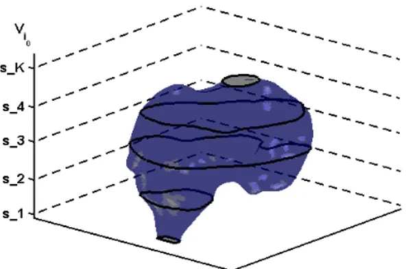
2.2 Example of Sparse Information Model for Volumetric Segmentation . . . 52
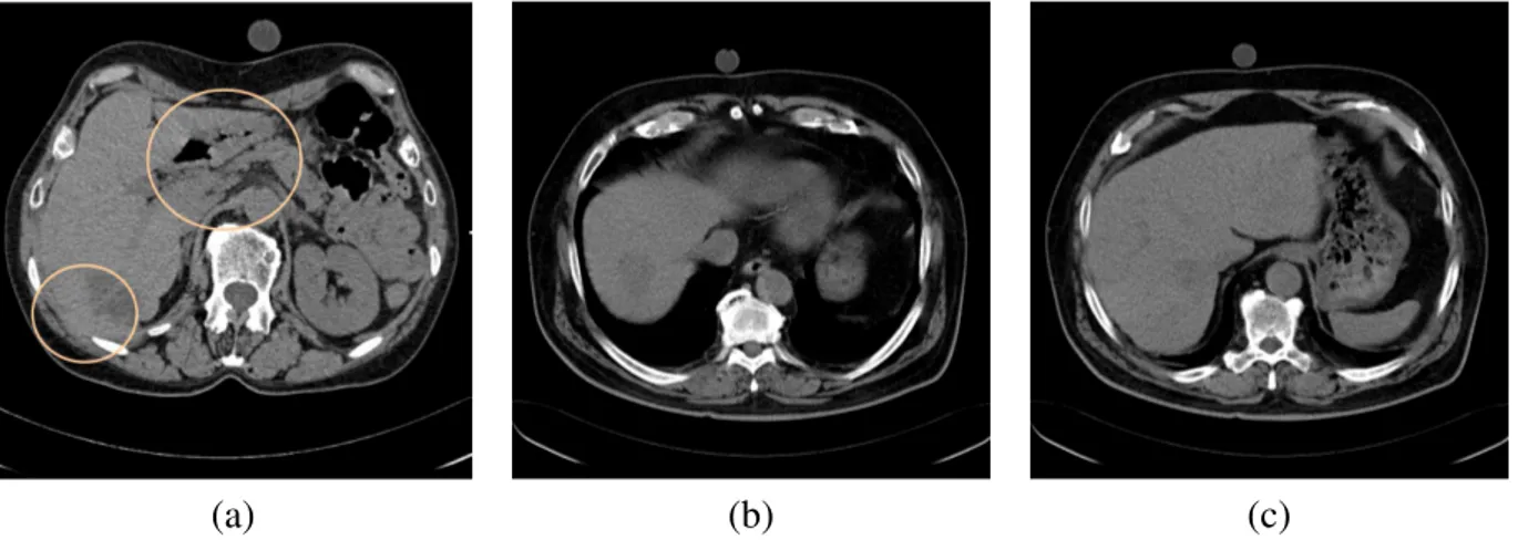
2.3 Liver slice with poor contrast . . . 55
2.4 Sparse Information Interpolation Energy . . . 58
2.5 Sparse Information Image Support . . . 60
2.6 Sparse Information Robustness . . . 61
2.7 Results of Dimensionality Reduction using Sparse Information Models. . . 64
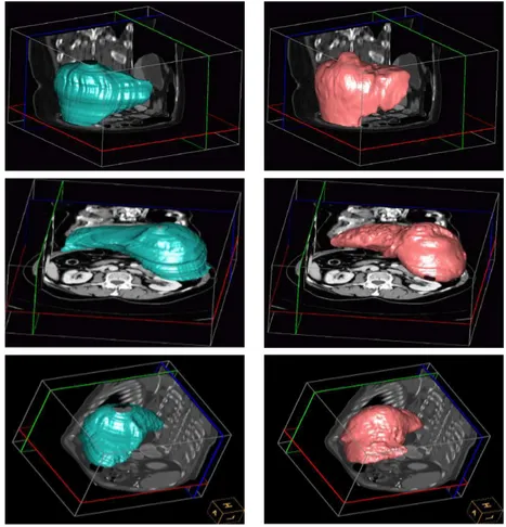
2.8 Examples of Livers Segmented using Sparse Information . . . 69
2.9 Four chambers view in ultrasound . . . 71
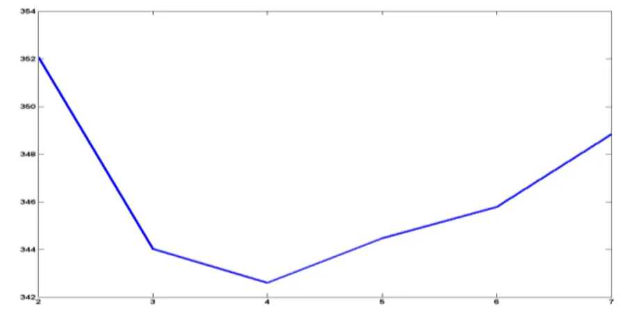
2.10 Schwarz Information Criterion for Ultrasound Sparse Segmentation . . . 74
2.11 RMS distance for Ultrasound Sparse Segmentation . . . 74
2.13 Sparse information model robustness to initialization. . . 76
2.14 Autoregressive interpolation robustness to initialization.. . . 77
2.15 3D RMA dataset benchmark . . . 79
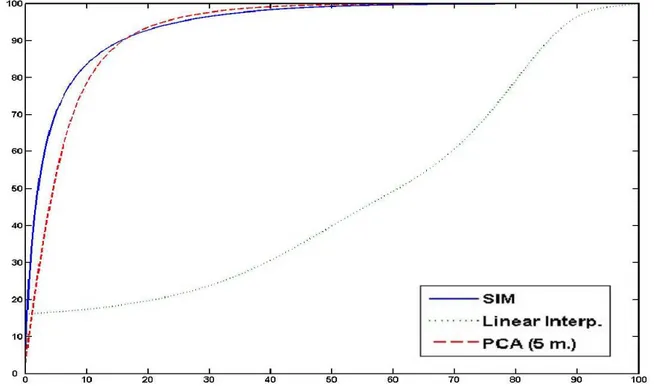
2.16 Cumulative Histograms of Reconstructed Surface Distances with respect to Ground Truth. . . 81
2.17 Representation of Range Data for Surface Reconstruction using Sparse Information 82 3.1 Registered training examples used for initial principal components analysis. . . 90
3.2 Vertical occlusion added to the original dataset . . . 93
3.3 Horizontal occlusion added to the original dataset . . . 93
3.4 Schwarz Bayesian criterion for AR sequential segmentation of ultrasound sequences. 98 3.5 Boxplot results of sequential segmentation of ultrasound images. . . 99
3.6 Comparison of ultrasound sequences segmented with AR with/out correction. . . . 100
3.7 Cross-correlation of PCA Coefficients for Left Ventricle Contours in Echocardio-graphy. . . 101
3.8 Sparse information model robustness to initialization. . . 102
3.9 Boxplot results of interpolation using the AR model. . . 103
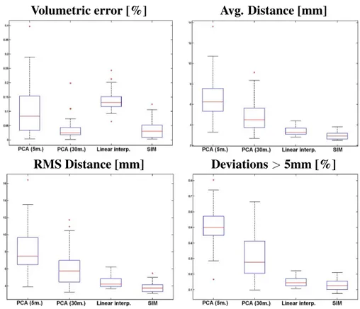
3.10 Comparison of Liver Segmentations using Different Techniques . . . 104
4.1 Visual Results of an Artery Sequentially Segmented . . . 113
4.2 Feature Space used to Model Vessels . . . 113
4.3 Examples of Pathologies for Coronary Arteries . . . 114
4.4 Overview of the Different Steps Involved in the Segmentation of Vessel with Par-ticle Filters . . . 115
4.5 Vessels are Segmented by the Kalman Filter . . . 116
4.6 Kalman Filter is Unable to Segment Bimodal Distributions . . . 116
4.7 Sequential Importance Resampling . . . 118
4.8 Principle of Vessel Segmentation Using Particle Filters . . . 121
4.9 3 Branchings Correctly Segmented by Particle Filters . . . 123
4.10 Vessel Cross-Section in Log-Polar view . . . 125
4.11 Vessel Cross-Sections Segmented by the Circular Shortest Path . . . 126
4.12 Comparison of Ground-Truth and Results Obtained with Particle Filters . . . 128
4.13 3D Visual Results of Real Cases Segmented by Particle Filters . . . 129
4.14 Synthetic Examples Segmented by Particle Filters . . . 131
4.15 Cerebral X-Ray and CT Angiographies . . . 133
4.16 The projected vascular structure and the distance map associated with it. . . 134
4.17 Corrupted X-ray image . . . 135
4.18 Condensation and Levenberg-Marquardt performances with respect to input noise . 136 4.19 Comparison of results obtained with condensation and Levenberg-Marquardt with noisy images . . . 137
4.20 (L) Comparison between Condensation and Levenberg-Marquardt method perfor-mance. (R) Registered vascular structure with 2D projection simulated from orig-inal CT data . . . 138
2.1 Comparative Study between PCA and Sparse Information Models for
Dimension-ality Reduction . . . 63
2.2 Quantitative Comparison for Liver Segmentation between PCA and Sparse Infor-mation Models . . . 67
2.3 Surface Reconstruction results using Sparse Information . . . 80
3.1 Tracking Results with non-Stationary Autoregressive Model of Walker Silhouette with Digital Occlusions . . . 94
3.2 Segmentation Results of Livers using Stationary Autoregressive Models . . . 103
4.1 Pixel intensity range for different organs coded on 12 bits. . . 126
4.2 Number of Branches Correctly Segmented by Particle Filters . . . 130
4.3 Quantitative Results of Synthetic Images Segmented by Particle Filters . . . 132
Contribution
Segmenter un objet dans une image num´erique consiste `a lab´eliser les pixels qui appartiennent `a cet objet et ceux qui appartiennent au fond. La segmentation est une ´etape pr´eliminaire `a l’analyse du contenu de l’image, et est n´ecessaire dans nombre d’applications telles que le diagnostique en imagerie m´edicale, ou la reconnaissance d’objet. Le nombre d’images `a interpr´eter ayant augment´e de fac¸on exponentielle ces vingt derni`eres ann´ees, l’analyse automatique est devenue une n´ecessit´e `a cause de contraintes de temps et d’argent. De plus, dans beaucoup de cas, une ´evaluation quan-titative pour le diagnostique ou la surveillance n’est possible qu’apr`es avoir d´elimit´e les contours de l’objet d’int´erˆet. Les r´ecentes avanc´ees dans ces domaines ont rendu possibles certaines appli-cations telles que: la s´ecurit´e et la vid´eosurveillance dans les lieux publics (a´eroports, hˆopitaux et stades sportifs), la reconnaissance automatique de visages pour l’identification ou la lutte contre la criminalit´e, le controle de trafic depuis l’analyse comportementale des clients dans les centres d’achat `a la gestion de trafic routier, l’´edition d’image et de vid´eo du dessin assist´e par ordinateur aux effets sp´eciaux de l’industrie des jeux et cin´ematographique, ou du diagnostique et planifica-tion de traitement en radiologie.
Les techniques de segmentation se basent sur l’information de l’image (aussi appel´ee sup-port de l’image dans cette th`ese) pour d´etecter soit les regions qui font partie de l’objet d’int´erˆet, soit les bords entre l’objet et le fond. Dans le contexte des images de sc`enes naturelles (e.g. les images m´edicales), la faible r´esolution des images et des donn´ees corrompues ou pathologiques rendent souvent n´ecessaires l’utilisation d’une connaissance `a priori `a propos de l’objet `a seg-menter. Cette connaissance `a priori est utilis´ee pour construire un mod`ele et contre-balancer les r´egions de l’image qui ne supportent que faiblement la segmentation ou la conduisent vers une so-lution fausse. Ces vingt derni`eres ann´ees ont vu beaucoup de techniques se d´evelopper autour de ce probl`eme, nottament les mod`eles de formes et d’apparence (intensit´e des pixels). Une analyse
de la distribution statistique de la forme et de l’apparence de l’objet r´eduit la complexit´e de la segmentation et guide la solution vers les formes les plus probables statistiquement.
Le travail pr´esent´e ici introduit comment des mod`eles statistiques peuvent ˆetre construits et exploit´es `a partir d’une quantit´e limit´ee d’information. Cette quantit´e limit´ee d’information (aussi appel´e information clairsem´ee) doit ˆetre s´electionn´ee avec soin afin qu’elle soit facilement identi-fiable dans l’image et permette une reconstruction efficace du reste de l’information. Puisque les images naturelles ont des r´egions qui supportent mieux la segmentation que d’autres, il est raison-able d’identifier ces r´egions dans l’ensemble d’apprentissage, et d’apprendre `a interpoler le reste de la segmentation, au lieu d’essayer d’extraire le contenu de l’image en incluant des r´egions qui sont notoirement pauvres en information ou qui conduisent au mauvais r´esultat. Puisque ces mod`eles statistiques peuvent ˆetre statiques ou non, nous avons examiner les deux cas. Les techniques les plus utilis´ees pour le suivi d’objet dans des s´equences d’images consistent `a isoler et suivre ses caract´eristiques, ou estimer le champ de d´eplacement appel´e flot optique qui lie une image dans la s´equence `a l’image successive. L’approche propos´ee dans cette th`ese est plus directe ; elle consiste `a mod´eliser le d´eplacement de l’objet d’int´erˆet `a partir de la connaissance `a priori. Dans la plupart des cas, les caracteristiques de l’objet sont d´ej`a connues (localisation, forme, apparence, ...), ainsi que son d´eplacement approximativement. En pr´edisant les caract´eristiques de l’objet dans des temps futures, sa segmentation devient plus pr´ecise et l’on peut mˆeme segmenter toute la s´equence d’images `a la fois si elle est disponible. Ces mod`eles de suivi peuvent mˆeme ˆetre utilis´es pour la segmentation classique avec une approche progressive. Dans ce cas, un temps fictif est introduit, et l’´etat de la solution `a un moment donn´e est utilis´e pour pr´edire le prochain ´etat. Enfin, la seg-mentation progressive qui consiste `a d´eterminer les caract´eristiques les plus probables de l’objet `a chaque pas de temps ne permet pas de r´esoudre certains probl`emes les plus difficiles. Pour l’un d’entre eux, nous proposons une nouvelle m´ethode qui consiste `a consid´erer les caract´eristiques de l’objet comme une variable al´eatoire et ´echantilloner l’espace de cette variable al´eatoire. Ainsi, des caract´eristiques faiblement probables `a un temps donn´e sont conserv´ees et peuvent donner lieu plus tard `a la solution correcte.
En travaillant `a Siemens Corporate Research, `a Princeton, NJ , quatorze certificats d’invention et brevets ont ´et´e d´epos´es, et les travaux relatifs `a cette th`ese ont ´et´e publi´es dans des conf´erences renomm´ees dans le domaine de la vision par ordinateur et de l’imagerie m´edicale:
Time-Varying Linear Autoregressive Models for Segmentation, Charles Florin, Nikos Paragios, Gareth Funka-Lea et James Williams, ICIP 2007, San Antonio, Texas, USA
Liver Segmentation Using Sparse 3D Prior Models with Optimal Data Support, Charles Florin, Nikos Paragios, Gareth Funka-Lea et James Williams, IPMI 2007, Kerkrade, Pays-Bas
Locally Adaptive Autoregressive Active Models for Segmentation of 3d Anatomical Structures, Charles Florin, Nikos Paragios, et James Williams, ISBI 2007, Arlington, VA, E-U
Globally Optimal Active Contours, Sequential Monte Carlo and On-line Learning for Vessel Segmentation, Charles Florin, Nikos Paragios, et James Williams, ECCV 2006, Graz, Autriche
Automatic Heart Isolation for CT Coronary Visualization using Graph-Cuts, Gareth Funka-Lea, Yuri Boykov, Charles Florin, Marie-Pierre Jolly, Romain Moreau-Gobard, Rama Ramaraj et Daniel Rinck, ISBI 2006, Arlington, VA, E-U
Registration of 3D angiographic and X-ray images using Sequential Monte Carlo sampling, Charles Florin, James Williams, Ali Khamene et Nikos Paragios, CVBIA 2005, pages 427-436, Beijing, Chine
Particle Filters, a Quasi-Monte Carlo Solution for Segmentation of Coronaries, Charles Florin, Nikos Paragios et James Williams, MICCAI 2005, pages 246-253, Palm Springs, CA, E-U
Automatic heart peripheral vessels segmentation based on a normal MIP ray casting technique, Charles Florin, Romain Moreau-Gobard et James Williams, MICCAI 2004, vol. 1, pages 483-490, Saint-Malo, France
Pr´esentation G´en´erale de la Th`ese
Chapitre 1: Revue de l’Etat de l’Art en Segmentation et Suivi d’Objet
Le premier chapitre effectue une revue des techniques les plus connues de segmentation et suivi d’objet. Il est divis´e en trois parties ; dans la premi`ere sont pr´esent´ees les m´ethodes sans mod`ele ou `a mod`ele de faible niveau. Les mod`eles `a faible niveau ne d´ependent que d’observations directes de l’image tels que l’intensit´e des pixels, les gradients, ... La seconde partie pr´esente les techniques se basant sur des mod`eles qui repr´esentent l’objet d’int´erˆet d’une mani`ere plus avanc´ee telles que des patrons, ou des distributions statistiques. Les techniques `a mod`ele contraignent l’information de l’image avec la connaissance `a priori afin de produire une solution au probl`eme de segmentation qui
soit plus robuste aux informations manquantes ou corrompues dans l’image. La troisi`eme partie pr´esente les m´ethodes de suivi et de segmentation s´equentielle. Globalement, il est int´eressant de remarquer que les techniques actuelles ne hi´erarchisent pas l’information selon le degr´e de support effectif qu’elle apporte `a la segmentation. Pour la segmentation, cela signifie apprendre `a partir de la connaissance `a priori quelles sont les r´egions de l’image qui supportent au mieux la solution. Pour le suivi d’objet, cela signifie mod´eliser les changements de charact´eristiques de l’objet au travers du temps. Finallement, il est constat´e que les techniques actuelles sous-utilisent les mod`eles d’incertitude de telle sorte que le r´esultat de la segmentation s´equentielle n’est que la succession des solutions locales les plus probables. Ces trois aspects sont examin´es en d´etail dans la suite de la th`ese.
Chapitre 2: Mod`ele `a Information Clairsem´ee pour la R´eduction de Dimension et de Complexit´e
Ce chapitre examine les mod`eles de segmentation `a partir d’information claisem´ee. L’image est divis´ee en r´egions, et une mesure est associ´ee `a chaque r´egion pour quantifier la fac¸on dont elle sup-porte la segmentation. Ensuite, est introduit un mod`ele qui n’utilise que les r´egions qui supsup-portent fortement la segmentation. Le reste de la solution est reconstruit `a partir d’une interpolation dirig´ee par un mod`ele. Apr`es une g´en´eralisation th´eorique, cette m´ethode est appliqu´ee `a trois probl`emes differents d’int´erˆet majeur en vision par ordinateur. Le premier de ces probl`emes est la segmen-tation d’objet dans une image volum´etrique, dans lequel le mod`ele `a information clairsem´ee est compar´e `a une technique bien connue de d´ecomposition lin´eaire afin de mesurer les b´en´efices de cette nouvelle approche en termes de r´eduction de dimension. Le second probl`eme est le suivi et la segmentation du ventricule gauche en ´echocardiographie, et montre l’efficacit´e de cette approche dans les cas de haute variance statistique. Une analyse statistique est men´ee sur les r´esultats de cette m´ethode et compar´ee `a la variabilit´e inter-experts. Finallement, le troisi`eme probl`eme est la reconstruction de surface `a partir de distances point´ees par laser, dans lequel la robustesse de la nouvelle m´ethode est analys´ee avec la pr´ecense de bruit sel et poivre.
Chapitre 3: Mod`eles de D´eplacement pour des Dynamismes non-Stationaires par Autoregression
Le troisi`eme chapitre introduit les mod`eles de d´eplacement appris `a partir de connaissance `a pri-ori, et pr´esente comment les adapter `a la vol´ee afin qu’`a la fois la repr´esentation des formes et celle des dynamismes soient mises `a jour avec l’information la plus r´ecente dans la s´equence.
En cons´equence, l’utilisation de mod`eles de d´eplacement n’est pas restreinte `a des d´eplacements qui fassent partie d’un ensemble d’apprentissage, telles que toutes les sc`enes naturelles par ex-emple. Ce concept est pr´esent´e avec des mod`eles autoregressifs lin´eaires par souci de simplcit´e math´ematique, et `a cause du grand nombre de cas couverts par ces mod`eles. Cette technique est appliqu´ee `a l’´etude de cas d’une silhouette d’un homme qui marche puis court. Des occlusions sont ajout´ees num´eriquements afin d’´etudier l’accumulation d’erreur. Cette m´ethode est ´egalement ap-pliqu´ee ´a des probl`emes stationaires pour mod´eliser toute la s´equence `a la fois. Enfin, elle est ´etendue `a une technique d’interpolation temporelle bas´ee sur la th´eorie de restauration de signaux audio.
Chapitre 4: Mod`eles d’Incertitude pour la Segmentation S´equentielle
Le quatri`eme chapitre pr´esente la derni`ere contribution de cette th`ese. Le probl`eme de segmen-tation de structures tubulaires dans des images volum´etriques est reformul´e comme un probl`eme de suivi en introduisant un temps fictif. Les charact´eristiques de ce tube `a un temps donn´e sont repr´esent´ees par une distribution statistique afin que non seulement la solution la plus probable soit d´etermin´ee, mais aussi d’autres solutions hypoth´etiques de plus faible probabilit´e. Dans le cas d’images de pathologies ou avec des artefacts d’acquisition, il est prouv´e que garder unique-ment les solutions les plus probables ne m´ene pas `a la solution globale correcte, alors que des solutions localement imparfaites peuvent mener `a la bonne solution globale. Cette technique est impl´ement´ee en effectuant un ´echantillonage s´equentiel al´eatoire, appel´e filtrage particulaire. Puis, afin de comparer le filtrage particulaire avec des techniques de descente du gradient couramment utilis´ees, un probl`eme statique et param´etrique est examin´e: le recalage 2D-3D.
Contribution
The segmentation of an object from a digital image consists in labeling the pixels that belong to this object and those that belong to the background, or alternatively in defining a boundary that encloses the object. Segmentation is a fundamental step to image content analysis whose outcome has numerous potential applications such as diagnosis in medical images or object recognition. The number of images to process in these fields have grown exponentially these past two decades, and have made computer-aided image analysis a major field of study because of time and finan-cial constrains. Furthermore, in most cases, quantitative assessment for diagnosis requires the delineation of the object of interest. Recent advances in this field have allowed new applications to appear such as: security and surveillance in crowded areas (airports, hospitals and stadiums security), automatic face recognition for identification and anti-terrorism, traffic control from cus-tomer behavior analysis in shopping malls to road traffic management, image and video editing from computer assisted design to movies special effects, cinematography, or diagnosis and therapy planning from radiology.
Segmentation techniques rely on image information (also called image support in this thesis) to detect either regions that are part of the object of interest, or edges between the object and the background. In the context of images that depict natural scenes (e.g. medical images), low resolution images and corrupted or pathological data often require prior knowledge about the object to segment. Prior knowledge is used to build a model and counter-balance image regions where insufficient support could mislead the segmentation. In the past two decades, many techniques have been developed to tackle this problem, which includes model priors based on shape or appearance (pixel intensities). A statistical distribution analysis of the object’s shape and appearance is used to reduce the segmentation problem complexity and guide the solution toward likely shapes.
The present work investigates how statistical models are built and exploited from a limited amount of information. This limited amount of information (also referred to as sparse information) has to be carefully chosen so that it is easily identifiable in the input image and could efficiently be used to reconstruct the remaining information. Since natural images have regions that support the segmentation task in a stronger way than others, it makes sense to identify these regions from prior knowledge, and learn how to express the remaining information used to represent the object instead of trying to extract content from image regions that are known to poorly support or mislead the segmentation. These statistical models may be either static or time-variant in cases where the object geometry changes according to some temporal process; we have investigated both. In image sequences, common approaches to object tracking consists in isolating and tracking features or estimating the velocity field called optical flow that wraps an image to the successive image. A more direct approach is proposed in this thesis; it consists in modeling the object of interest’s motion using prior knowledge. In most cases, one already knows the characteristics (e.g. location, shape, appearance, ...) of the object to track and roughly how it moves. By predicting the object’s characteristics in future frames, one may segment it more accurately and may even segment the whole sequence of images at once if it is available. Models for tracking in images sequences may even be applied to regular segmentation by progressively solving this problem. A virtual timeline is introduced and the solution’s state at one time is used to predict the next state. Finally, progressive segmentation that consists in determining the most probable object features at each time step does not allow the solving of some of the most difficult problems. Such cases refer to important deformations of the object that cannot not be represented by simple linear models. In such cases a more complex probabilistic interpretation of the object dynamics is required. To this end,, we propose a novel approach that consists in representing the object’s features as a random variable and sampling the feature space. Thus, features that have a low probability to be exact at a given time step are kept and may correspond to the correct solution at a later time step.
While working for Siemens Corporate Research, Princeton NJ, fourteen invention disclosures and patents relevant to the present thesis were filed. Also, relevant publications were presented in renowned computer vision and medical images conferences:
Time-Varying Linear Autoregressive Models for Segmentation, Charles Florin, Nikos Paragios, Gareth Funka-Lea et James Williams, ICIP 2007, San Antonio, Texas, USA
Liver Segmentation Using Sparse 3D Prior Models with Optimal Data Support, Charles Florin, Nikos Paragios, Gareth Funka-Lea et James Williams, IPMI 2007, Kerkrade, Pays-Bas
Locally Adaptive Autoregressive Active Models for Segmentation of 3d Anatomical Structures, Charles Florin, Nikos Paragios, and James Williams, ISBI 2007, Arlington, VA, USA
Globally Optimal Active Contours, Sequential Monte Carlo and On-line Learning for Vessel Segmentation, Charles Florin, James Williams, and Nikos Paragios, ECCV 2006, Graz, Austria
Automatic Heart Isolation for CT Coronary Visualization using Graph-Cuts, Gareth Funka-Lea, Yuri Boykov, Charles Florin, Marie-Pierre Jolly, Romain Moreau-Gobard, Rama Ramaraj and Daniel Rinck, ISBI 2006, Arlington, VA, USA
Registration of 3D angiographic and X-ray images using Sequential Monte Carlo sampling, Charles Florin, James Williams, Ali Khamene and Nikos Paragios, CVBIA 2005, pages 427-436, Beijing, China
Particle Filters, a Quasi-Monte Carlo Solution for Segmentation of Coronaries, Charles Florin, Nikos Paragios and James Williams, MICCAI 2005, pages 246-253, Palm Springs, CA, USA
Automatic heart peripheral vessels segmentation based on a normal MIP ray casting technique, Charles Florin, Romain Moreau-Gobard and James Williams, MICCAI 2004, vol. 1, pages 483-490, Saint-Malo, France
Thesis Overview
Chapter 1: Review of Prior Art in Segmentation and Tracking
The first chapter reviews the most common techniques for segmentation and tracking. It is divided into three parts; in the first part, model-free and low level models are presented. Low-level mod-els only rely on direct observations from the image such as pixel intensities, image gradients, ... The second part introduces model-based techniques that represent the object of interest in a more advanced fashion using templates, or statistical distributions. Model-based techniques integrate the image information with prior knowledge in order to produce a solution to the segmentation problem that is more robust to missing or corrupt image data. The third part is devoted to tracking techniques and sequential segmentation. Overall, it is noted that current techniques do not hier-archize input information with respect to the amount of information they effectively provide for solving the segmentation problem. For segmentation, this means learning from prior knowledge
which image regions best support the solution. For tracking, this means modeling the changes of the object’s characteristics across time. Finally, current segmentation techniques underuse uncer-tainty models so that the solution of a sequential segmentation is the succession of the most likely individual solutions. These three aspects are investigated in the three following chapters.
Chapter 2: Sparse Information Models for Dimensionality and Complexity Reduction
This chapter examines segmentation models based on sparse information. The input image or shape is divided into regions, and a measure is associated to each region to quantify how it sup-ports the segmentation. Then, a model that uses only the best supported regions is introduced. The solution’s remaining is reconstructed using a model-driven interpolation. After a theoretical introduction, this method is applied to three different problems of significant interest in computer vision. The first problem is organ segmentation in medical volumetric images, in which the sparse information model is compared to a common linear decomposition technique to test the benefits of the novel approach in terms of dimensionality reduction. The second problem is tracking and segmentation of the left ventricle in ultrasonic sequences, and proves the effectiveness of this ap-proach in case of high statistical variance. A statistical analysis is conducted to compare the sparse information models with inter-expert variability. Finally, the third problem is surface reconstruc-tion from laser pointed distances, in which the robustness of the novel method is analyzed in the context of salt and pepper input noise.
Chapter 3: Motion Models for Non-Stationary Dynamics via Autoregressive Models
The third chapter introduces motion models learned from prior knowledge and presents how to adapt them on-the-fly so that both the representation of the shapes and the dynamics are updated with the newest information available in the sequence. Consequently, the use of motion models is not constrained to behaviors that are part of the learning set, as merely all natural scenes. This concept is presented with linear autoregressive models for the simplicity of the mathematics and the high number of cases covered by such models. This technique is applied to the study case of a walking silhouette that starts to run. Digital occlusions are added to test the accumulation of errors. This technique is also applied to stationary problems to model the motion in all the sequence at once. It is then extended to a temporal interpolation technique based on audio signal restoration theory.
Chapter 4: Uncertainty Models for Progressive Segmentation
The fourth chapter presents the last contribution of this thesis. In the context of tubular structures segmentation, the multi-hypothesis framework is introduced and implemented with a sequential random sampling procedure called particle filters. Segmentation of tubular structures in volumetric images is reformulated as a geometric tracking problem using a virtual timeline. The characteris-tics of the tube at one point in the timeline are represented by a statistical distribution so that not only the most likely solution is preserved but also hypothetical solutions of lower probabilities. In the case of pathological data or images with acquisition artifacts, one can claim that the approach consisting in keeping only the most probable solution fails, while some of the less probable solu-tions may give rise to the correct global solution. This technique is implemented using a sequential Monte-Carlo sampling method called particle filters. The outcome of this method is used to seg-ment highly non-linear structures such as the coronary arteries. Then, in order to compare this framework with commonly used gradient descent approaches, it is extended to a static parametric problem: 2D-3D registration.
Learning to Segment and to Track
Abstract – This chapter intends to review the scientific literature in segmentation and tracking with and without models
and prior learning. First, techniques based solely on low level information (pixels intensity, image gradient, ...) are presented when the image is modeled by a continuous function and when it is represented in a discreet way. Second, model-based methods are introduced starting by rigid models of few parameters, with none or little adaption, to the soft models that represent the object of interest using probability distributions. Then, these soft models are integrated into low level techniques. Finally, in the context of image sequences, common frameworks combining stochastic modelling and time-series are introduced.
1.1 Introduction
Object segmentation is equivalent to labelling the pixels in the image that belong to the object and those that belong to the background. Segmentation is the prime step of content extraction and content analysis; therefore a tremendous effort is put on developing algorithms that best segment with respect to human experts, as quickly as possible.
One may distinguish different ways to segment an image. The first is to analyze the pixels intensity value directly and to group the pixels according to intensity similarity, texture or higher order statistical properties and/or detect strong intensity gradients. This method regroups the model free and low level model techniques. The second method is to use a model (e.g. appearance or shape) and to detect the image regions that best match the model. The third is to transform the segmentation problem into a dynamic problem in which the solution (the labeling of the pixels belonging to the object of interest) is progressively achieved using Bayesian processes. When the input images form a time sequence, the object’s segmentation across time is called tracking.
1.2 Model-Free and Low-Level Model Based Segmentation
1.2.1 Active Contours Model Active contours and snakes
Active contours and snakes models were first introduced by Kass, Witkin and Terzopoulos in 1987 [104]. In many cases, an object distinguishes itself from the background by a boundary: a strong edge, a particular color, ... A general way to note that is to call g a function to minimize locally. Typically, if an object is defined by a strong edge, g is inversely proportional to the image gradi-ent. In the following, the object boundary is denoted by a curve C, parameterized by p ∈ [0, 1]. The curve C that defines the object’s boundary theoretically minimizes the following energy E in equation (1.1) that combines a smoothness term and an image term:
E(C) = Z 1 0 α ° ° ° °∂C∂p ° ° ° ° 2 + β ° ° ° °∂ 2C ∂p2 ° ° ° ° 2 | {z } smoothing term + λg(C(p)) | {z } image term dp. (1.1)
The smoothness term stands for regularity/smoothness along the curve and has two components (resisting to stretching and bending). The image term g guides the active contour toward the desired image properties (strong gradients). Other terms may be added to take into account user-defined points or other external constraints such as prior knowledge [83][204][192]. External constraints were introduced because the need for models was felt very early. The basic approach for active contours is a local optimization, which makes the method quite sensitive to local minima, occlusions and missing/corrupted data.
The general approach for active contours is to consider a discrete variant of the curve using a number of control points, and evolve that curve C by minimizing the energy in equation (1.1) at each time step until convergence. Due to the fact that this method was a significant breakthrough in image segmentation, a large part of the following work in the domain is mainly influenced by the idea of designing ever-better energies, to minimize them by more and more efficient numerical schemes to get the globally optimum segmentation result, with respect to that particular energy and that particular scheme. However, this expression may lead to poor results and the snake may shrink to a point in certain regions of the image. In [36] et al. introduced a balloon force ν1 that
avoids the shrinking when no edge information is present.
The main advantages of Active Contour models are their low complexity, the fact that it is easy to introduce prior knowledge, and that they could account for open as well as closed structures. It is also a well established technique, and numerous publications are available. Finally, user interactiv-ity is naturally handled by introducing an extra energy term in the equation. However, they suffer from being myopic (only local image information is taken into account), cannot handle topological changes and the solution to the segmentation problem depends on the selected parameterization.
Geodesic Active Contours
Caselles et al. [31] and Kichenassamy et al. [105][106] reformulated the active contour equation in a more rigorous way starting back from the snakes equation (equation (1.1)) and omitting certain terms: E(C) = α Z 1 0 ° ° ° °∂C(p)∂p ° ° ° ° 2 dp | {z } intrinsic energy +λ Z 1 0 g (|∇I (C(p))|) dp | {z } extrinsic energy . (1.2)
1ν is generally a small positive constant designed to inflate the curve like a balloon to prevent it from shrinking
By reparameterizing the curve using the Euclidean arc-length ds, ° ° °∂C(p)∂p ° °
° dp = ds, and using the Malpertuis’ Principle, Caselles et al. proved in [31] that, when α = 0, to find the curve C that minimizes equation (1.2) is equivalent to find the curve of minimal length Lg in a Riemannian
space that depends on the function g: Lg =
Z L(C)
0
g (|∇I (C(s))|) ds, (1.3)
where L (C) is the Euclidean length of the curve C. The curve of minimum Riemannian length is determined by taking the first derivative of equation (1.3), and using an iterative method with time step ∂t [30][35][125][107]: ∂C ∂t = g (|∇I (C)|) KN| {z } boundary force − (∇g (|∇I (C)|) .N ) N | {z } refinement force . (1.4)
The main drawbacks of active contours are their sensitivity to initialization (the curve always converges to the nearest local minimum), to parameterization and to the chosen topology. If a topology change occurs (e.g. the curve has been initialized as one single piece, but the actual object to segment is composed of two disjoint pieces), a complex heuristic has to break the curve into multiple pieces and reparameterize each piece independently. To overcome this drawback, level-sets were introduced by Dervieux and Thomasset [58][57], before been rediscovered independently by Osher and Sethian [137] for flame propagation, then applied to image segmentation by Malladi et al. in 1995 [126]. However, this expression may lead to poor results and the curve may shrink to a point in certain regions of the image. In order to cope with that, a force similar to the balloon [36] was also introduced for the case of geometric active contours.
∂C
∂t = g (|∇I (C)|) (K + ν) N − (∇g (|∇I (C)|) .N ) N . (1.5)
Implicit Active Contours: Level Sets
The basic idea of level sets is to represent a given contour C by the zero level-set of a function2 ψ
(see figure (1.1)) , as written in equation (1.6) where Γ (resp. ¯Γ) is the image region inside (resp. 2the Euclidean distance function is used in most of the cases due to certain desired geometric properties
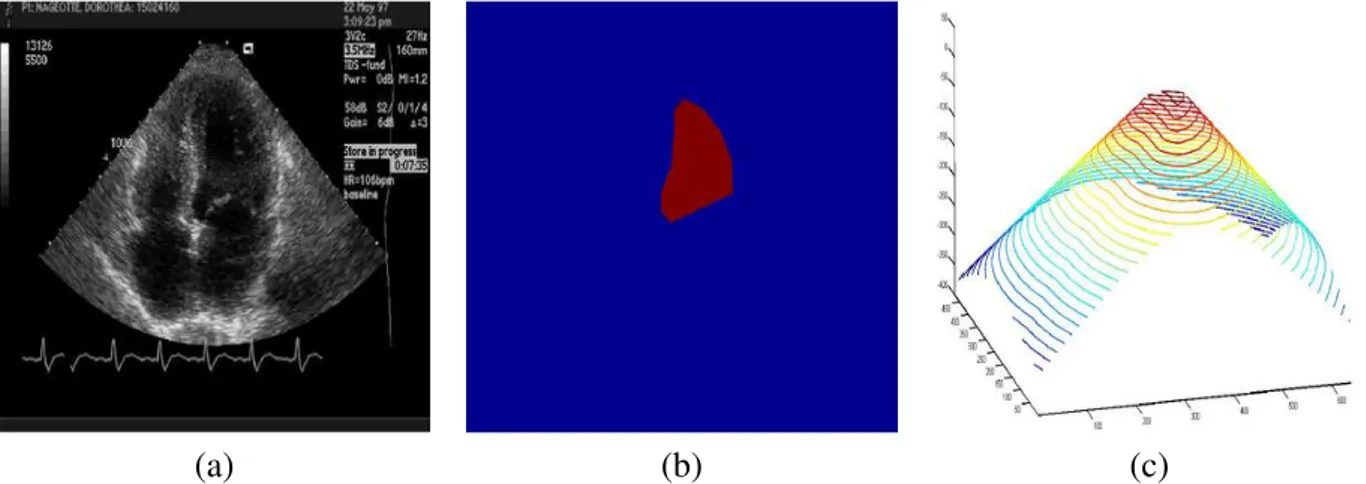
(a) (b) (c)
Fig. 1.1: Distance function that represents a shape (blue curve), positive inside the shape and negative
outside. (a) Original image. (b) Binary shape. (c) Distance function isolines.
outside) the object, and D(x) is the Euclidean distance between point p and the curve C:
ψ(p) = 0 , p ∈ C +D(p) > 0 , p ∈ Γ −D(p) < 0 , p ∈ ¯Γ (1.6)
One can embed in a straightforward fashion [137] the flow described in equation (1.4) in the level-set framework as described in equation (1.6), toward obtaining the following partial derivative equation that guides the propagation of ψ:
∂ψ
∂t = g (|∇I (C)|) K |∇ψ| + ∇g (|∇I (C)|) .∇ψ (1.7)
The popularity of level-sets method is largely due to the simplicity with which one may im-plement them. They do not require any specific parameterization, and implicitly handle topologi-cal changes. By a snow-ball effect, an abundant literature [167][141] reviews their mathematical convergence and stability as well as their solution existence and uniqueness, which leads to the level-sets been even more popular.
Region-based active contours started with the work of Zhu and Yuille in [203] where an energy formulation for segmentation of multiple regions was derived from a Bayesian/minimum descrip-tive length (i.d. posterior probability) expression. Then, Chan and Vese introduced in [33] a
multi-region scheme where each region was defined by the logical combination of several level-set functions’ sign. This expression guarantees only log(n) level-set functions are necessary to repre-sent n regions. This scheme was reformulated for the geodesic active contours in [144] under the name of geodesic active regions. In [198], Yezzi et al. reformulated the multi-object segmentation using a coupled evolution of any arbitrary number of geodesic active contours that is obtained from the definition of binary and trinary flows.
Geodesic active contours aim at representing the segmentation problem in an energetic fashion and optimizing the solution with partial derivative equations. However, the energy terms cor-respond to a low level model (on curvature, gradient structure, pixels intensity, ...) that, when established once and for all, may poorly fit the image and let the active contour converge to a local solution. To overcome that issue, Juan, Kerivan and Postelnicu [102] propose to add a simulated annealing procedure. Paragios [145] and Rousson [156] use statistical models of shape and ap-pearance that result in softer constrains for the active contours. For more details about level-sets, variational methods and implementations one may refer to [136].
1.2.2 Markov Random Fields and Gibbs Distributions
The probabilistic nature of image acquisition, noise and motion often drive the segmentation to-ward a low-level statistical model. In this case, instead of representing the solution by a continuous curve and solving partial derivative equations to determine the solution of minimal energy, one de-scribes the probability measure that associates the segmentation to a likelihood given the low-level model’s parameters (often based on pixels intensity) and the input image. Different techniques exist to determine the most likely solution. One consists in associating an energy function to the probability function and solving partial derivative equations (see previous sections). Another con-sists in sampling the random variable space and estimate directly the probability density function (see particle filters in section (1.4) for instance). A third solution consists in using Gibbs distribu-tions, Markov random fields (MRF for short) equivalence, for segmentation.
The basic idea of MRF is to divide the image into homogeneous regions with respect to certain parameters [78][139][13][54]. To that end, it is assumed a random variable z describes the ob-served (corrupted) image, a random variable x describes the label of the image regions (i.e. object, background, and so on) and a third random variable y is related to the (a priori unknown) charac-teristics of each region. The main idea is to determine the labeling x and characcharac-teristics y that best
fit the image z, or in other words to maximize the a posteriori probability: p (x, y|z) = p (z|x, y) p (x, y)
p (z) . (1.8)
The above equation (1.8) is referred to as the Bayesian rule equation, and relates the posterior probability p (x, y|z) to the conditional p (z|x, y) and prior p (z) probabilities.
MRF uses stochastic relaxation and annealing to generate a sequence of random variables that converges toward the maximum a posteriori3. An energy is defined by the negative logarithm of
the posterior probability function
E = −log (p (z|x, y)) − log (p (x, y)); the parameters {x, y} are locally adapted in the image to maximize this energy. The amplitude allowed for those changes are controlled by the annealing temperature parameter T that slowly decreases with respect to the number of iterations.
This technique has many advantages over hard constrained energies, especially in the pres-ence of noisy images that do not fit any pixels intensity model from prior knowledge. However, simulated annealing avoids certain local minima, but MRF remains a local optimization and the optimum solution cannot be guaranteed in a finite amount of time. In certain problems (denoising for instance), a local solution is sufficient; in others, a global minimum is critical. That is the reason why more efficient numerical schemes that guarantee a global solution are investigated. One example is the max flow/min path principle which has emerged in computer vision using an efficient implementation like the graph-cuts.
Although not exclusively used for computer vision, other discrete optimization techniques are of particular interest. Among them, dynamic programing plays a significant role. Dynamic pro-graming consists in dividing a general problem into a set of overlapping problems, iteratively solving each subproblem and recomposition the general solution. An important example of dy-namic programing is provided by Dijkstra [63] for computing shortest paths on a directed graph with non-negative edge weights, such as an image.
Belief propagation networks are a particular instance of belief networks used to optimize one or several probability distribution functions (such as the one in equation (1.8)) using graph theory. A particular example is the expectation-maximization algorithm [53] that is used to iteratively estimate a model’s parameters to maximize the likelihood of that model given observations.
Last, linear programming [50] aims at solving linear minimization problems subject to con-straints. A popular solution to the linear programming problems is given by the simplex algorithm [50]. Another algorithm of the same name, also called the downhill simplex algorithm is intro-duced by Nelder and Mead [130], and consists in iteratively estimating the solution for different values of the variables and modifying the worst set of variables according to the other possible estimated solutions.
Graph-Cuts
Graph-cuts is a very active field of study that is applied to different problems of computer vision such as segmentation [21][171][189][197][22], image restoration [23], texture synthesis [113] or stereo vision [159][109]. Let G = hV, Ei be an undirected graph whose set of vertices is noted V and contains two special nodes called terminal, and whose set of edges is noted E and has non negative weights we, ∀e ∈ E. A cut, noted C, is a subset of edges C ∈ E that partitions the original
set E in two such that each partition has one and only one terminal node. The cost of the cut |C| is the sum of the edges in C:
|C| =X
c∈C
wc. (1.9)
The graph-cut algorithm consists in finding the cut of minimal cost, and several implementations exist to determine such a cut in a polynomial time (e.g. max-flow and push-relabel [37]). It is of particular interest in the context of segmentation, where each image pixel represents a vertice in the graph, and each edge’s weight is related to the relationship between two pixels intensity. For instance, if the edge’s weight weij between two vertices/image pixels ei and ej is defined as
weij =
1
1 + |I(ei) − I(ej)|
, (1.10)
where I(ep) is the image intensity for the pixel ep, the minimum cut includes vertices/image pixels
that have a low weight weij, that is neighboring pixels that are very dissimilar. In [22], Boykov and
Kolmogorov used graph-cuts to solve a geodesic problem and to include the types of energy that were previously solved using PDEs.
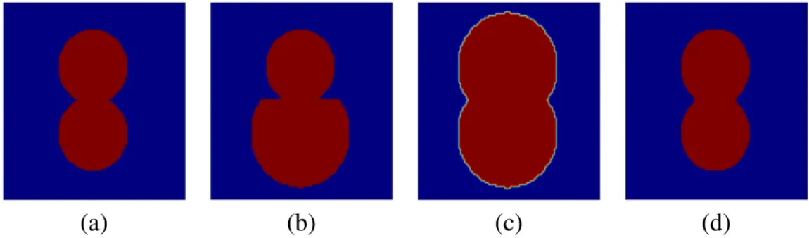
(a) (b) (c)
Fig. 1.2: (a) Original image (b) Template to match using the original image (c) Result of matching
1.2.3 Advantages and Drawbacks of Model Free Segmentation
With model free and low-level model techniques, one does not need to construct a model for the object of interest, which was a considerable advantage when data was not as widely available as it is now. In the particular context of organ segmentation in medical imaging, the inter patient variability of shape and appearance due to various image qualities and pathologies make certain modeling hazardous. The model free techniques are also often simpler to implement and may be quicker to compute. On the other hand, now that imaging data is commonly accessible (in 2005, about 60 millions CT and 1 million PET scans were performed in the US), robust models may be built to direct the segmentation.
1.3 Model-Based Segmentation
Template Matching
The simplest and most straightforward way to use a model for segmentation is template matching. Template matching consists in optimizing few parameters (position, rotation angle, scale factors) so that a template best matches the image (see figure (1.2)) according to a certain image measure whose global minimum corresponds to the best template alignment. If the only parameters to be optimized are position, rotation angle, scale factors, the template is called rigid template. This optimization is usually performed either using exhaustive search or gradient descent. For further
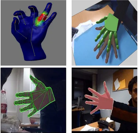
Fig. 1.3: An articulated model of the hand controlled by parameters to control angles and lengths. Courtesy
of M. de la Gorce [52].
investigation, one may refer to [26] to study the effectiveness of exhaustive search and template matching in the particular context of watermarking and image security.
Unlike rigid templates, deformable template and articulated templates are models that can be adapted depending on parameters. An example is given in figure (1.3) where the stick-man shape is controlled by few parameters to adjust the members angle and length to the input image. Articulated models are of particular interest for surveillance and behavior analysis [94]. In the context of medical image analysis, deformable organisms [85] combine sensors and a framework to optimize (deform) a template (organism) with respect to the image.
In many applications, the templates are derived from physical data in a straightforward way. However, in most cases, the templates cannot be defined explicitly, but have to be learned from prior knowledge. A solution consists in establishing a low-dimension basis onto which the object to segment are projected.
1.3.1 Decomposition using Linear Operators
A second approach is to represent the object’s model (shape and/or appearance) Y in a high dimen-sional space, then project the object’s model onto a lower dimension feature space, and optimize the feature vector X with respect to the image measure:
X = (g1(Y), g2(Y), ..., gm(Y)). (1.11)
In the following, different choices concerning the linear operators gis are exposed.
Linear discriminant analysis (or LDA) consists in finding the projection space that best sepa-rates two classes/exemplars p (X|Y = Y1) and p (X|Y = Y2). LDA commonly relies on Fisher’s
linear discriminant [72] and assumes the probability density functions (pdfs) are Gaussian with means Y1 and Y2 and the same covariance Γ. Fisher’s discriminant S is the ratio of the two
variances between and within the two classes Y1and Y2 after been projected along the vector w:
S = σ 2 between σ2 within = ¡ w.Y1− w.Y2 ¢2 2wT.Γ.w (1.12)
It can be shown that the vector w that maximizes the Fischer ratio is w = 1 2Γ −1.¡Y 1− Y2 ¢ . (1.13)
LDA is commonly applied to classification and recognition problems [10]. In a first step, a training set of samples is gathered to estimate the classes distribution properties (mean and variance). Then equation (1.13) is applied to determine the optimal projection.
Recent developments in LDA include a probabilistic LDA [96] that generates a model to extract image features and automatically assigns a weight to each feature according to their discriminative power.
Principal component analysis (PCA) [38] [186] assumes a Gaussian distribution of the train-ing samples. The main idea of PCA is to re-write a high dimensional vector Y as the sum of a mean vector Y and a linear combination of the principal modes of variation (see figure (1.4). Eigenanalysis of the covariance matrix is used to determine the orthogonal basis formed by the matrix eigenvectors, and the eigenvalues associated to them. This orthogonal basis is composed by
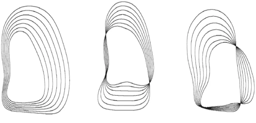
Fig. 1.4: Three principal modes of shape variations for the left ventricle in echocardiography.
the modes of variation, and the variations amplitude is given by the eigenvalues associated to each eigenvector/mode.
Let {Yi, i ∈ [|1, N |]} be the set of high dimensional vectors, Y be the mean of these vectors,
and Γ = [(Y1− Y)(Y2− Y)...(YN− Y)][(Y1− Y)(Y2− Y)...(YN − Y)]T be the covariance
matrix. Given that Γ is a symmetric real positive definite matrix, its eigenvalues are noted λ1 >
λ2 > ... > λN > 0 and the corresponding eigenvectors {Ui, i ∈ [|1, N |]}. Noting Λ the diagonal
matrix composed by the eigenvalues, and U = [U1U2...UN],
Γ = UΛUT. (1.14)
Any centered vector (Y − Y) may be projected onto the eigenvectors orthogonal basis using the similarity matrix U such that
Y − Y = UX, or noting X = [x1...xN]T, Y = Y + N
X
q=1
xqUq. (1.15)
However, in practical cases, many eigenvectors relates to small eigenvalues (compared to the largest ones); that means these vectors relate to low amplitude variations. Therefore it makes sense to draw a threshold and keep only the eigenvectors whose linear combination approximates up to p percent of the total variation.
However, in some cases, the Gaussian distribution of the data does not stand. PCA extensions have been proposed to solve these cases, the most noticeable of which is Kernel PCA. Another decomposition technique that has been developed for non-Gaussian distributions is the independent component analysis.
Independent component analysis (ICA) [95] aims at decomposing the input signal into decor-related non-Gaussian components. Given a signal Y, ICA retrieves the underlying decordecor-related non-Gaussian signals Si (called sources) such that Y =
PN
i=1AiSi by optimizing a cost function
(neg-entropy, kurtosis, ...) that is minimal when the sources are the farthest away from Gaussian distributions. Among the several methods that exist depending on the cost function, the prominent ones are FastICA [15], InfoMax [11] and JADE [28].
In a practical case, the multiple dimensions of Y are often correlated which makes the ICA de-composition theoretically impossible. For that reason, the signal is ”whitened” by estimating a lin-ear transformation L such that Y0 = LY and the transformed signal auto-correlation E[Y0TY0] =
I. This property is achieved with L =pE[YTY]−1 since E[Y0TY0] = E[YTLTLY] = I.
It is worth noting that, unlike PCA, ICA does not provide any ordering of the different com-ponents; therefore, ICA’s application to dimensionality reduction is not straightforward. In [187], Uzumcu et al. investigate the ordering of the sources for dimensionality purposes. LDA, PCA and ICA retrieve independent components that are intrinsic to the input signal and project the signal onto these components. Another way to proceed is to project the signal onto a canonical orthogonal basis of the functional space.
1.3.2 Decomposition using Non-Linear Operators
Fourier descriptors Let us assume a shape is represented in a parameterized way: Y(p), p ∈ [0, P ]; then, a Fourier analysis may be run over that input signal to retrieve the Fourier coefficients uk, so that the Fourier transform of the input signal bY is written as:
b Y(ν) =
Z ∞
t=0
or, sampling the shape function on N points, FFT is used to retrieve the discrete FD uk= N X k=1 Y(p)e−2πjkpN. (1.17)
In the context of shape analysis, these Fourier coefficients are referred to as Fourier descriptors (FD). FD are used in the context of shape classification [112] and denoising. No need to say that the FD depend on the choice of shape representation; for a comparative study of FD with different shape signatures, one may refer to [201].
Radial basis functions (RBF) [29][64][121][110] is another decomposition basis in the func-tional space. Just like FD, RBF decomposes the input signal Y(p) into a linear combination of primitive functions called kernels ρ:
Y(p) =
N
X
i=1
akρ (|p − ck|) , (1.18)
where the ckare called basis function centers.
Zernike moments have been proposed by Teague [177] to decompose a discrete image. Teague introduced a set of complex polynomials that form an orthogonal basis onto which an image (ap-proximated by a piecewise function) is decomposed. The projection of the image function on a particular Zernike polynomial is called a Zernike moment. The set of moments characterizes an image, therefore Zernike moments are of particular interest for image retrieval [132], denoising [9] and image classification [193]. The main limitation of these methods is that establishing a con-nection between the prior model and the image domain where the data support is available is not straightforward.
1.3.3 Prior Models for Geodesic Active Contours
Geodesic active contours (see section (1.2.1)) offer two main advantages: they can be embedded in the level-sets framework for an implicit shape representation, and additional energy terms can be introduced to the equation (1.4). These extra energy terms may be intrinsic to the shape (curvature, length, ...) or extrinsic (e.g. referring to the image or to prior knowledge). If a shape constrain is available, it is added as an extrinsic energy (e.g. the L2 distance between the current solution’s
level-sets and the prior constrain’s).
Since the level-sets are local optimization techniques, they are sensitive to initialization. Con-sequently, many model based methods [44][140] use a prior about the initial contour’s location, while others [30][105] use geometric models. Active shape models [38][186] use the modes of variation to constrain the shape evolution during the energy minimization. These modes of varia-tion are computed from prior knowledge by using PCA built from prior knowledge. In this basis, a shape is characterized by its distance to the mean shape along statistical modes of variation. How-ever, the shapes’ distribution on the modes may have very different variances that depend on the Eigenvalues of the covariance matrix (see section (1.14)). Thus, instead of using the Euclidean distance between the solution’s level-sets Y1 = {x1i} and the prior constrain’s Y2 = {x2i}, the
Mahalanobis distance is preferred:
Dmahal(Y1, Y2) =
sP
iλ2iP(x1i − x2i)2 iλ2i
. (1.19)
In [114], prior statistical shape analysis is combined with the geodesic active contours to con-strain the solution to the most likelihood solutions. When the prior dataset’s samples distribution in the PCA space does not fit a Gaussian, a solution consists in using a kernel distance in the PCA space [155], or in using a kernel method for dimensionality reduction [48][44].
1.3.4 Model-Based Segmentation Limitations
Compared to model-free segmentation, model based segmentation uses a priori knowledge mostly in the geometry space about the object to detect. This makes the segmentation process generally more robust but also introduces two main limitations. The first inherent limitation is the constraint one introduces by using a model. By limiting the segmentation to certain degrees of freedom, the role of local variations and image support is diminished. Also, in most cases, models are built from training sets where the available information (geometry and apperance) is treated equally, regardless of the image support. This problem is addressed in chapter2where a method is proposed to build a model on carefully chosen sparse information. Furthermore, the models presented in section (1.3) are time-invariant and are insufficient to solve tracking problems such as the one presented in chapter3. Last, in the context of optimization in time or space, the global solution may not just consist of the collection of locally most likely solutions. Since only the optimal solution
is looked for at each time step, or space scale, and no uncertainty model is used to represent other potential solutions, nothing guarantees the global solution is achieved when the full time or space information is considered. This issue is dealt with in chapter 4, where a segmentation problem is turned into a geometric tracking problem, and an uncertainty model is integrated into the segmentation framework.
1.4 Bayesian Processes for Modeling Temporal Variations
Many segmentation problems contain a time variable either real or virtual. A simple geometric model does not contain time information, which has to be modeled aside. This section introduces time sequence models starting from regression on deterministic variables, then presenting para-metric and non-parapara-metric models for random variables with and without linear state transition.
Autoregressive models. Let Xtbe a state variable at time t, and Ytbe the observation variable.
The general form of regression is a function f such that
Xt= f (Xt−1, Xt−2, ...Xt−p, Yt−1, ...Yt−q). (1.20)
However, many physical time-series are approximated using autoregression laws such as: Xt= A[Xt−1TXt−2T...Xt−pT] + W + ², (1.21)
such that the random noise ² is zero-mean with minimal covariance determinant. This regression law is established from prior knowledge and used to predict and constrain future states. In a general context, the regression law is not updated, therefore this technique is unable to sustain variations in the dynamic system.
The success of autoregressive (AR) models lies in the vast literature dealing with the subject and their easy implementation. However, AR models are mono-modal and poorly suit natural scene problems where the objects to track rarely moves according to one single time-invariant mode. Consequently, either a complex heuristic is developed to mix models, or Markov fields are introduced for multimodality, such as in [1].
seg-mentation using PCA (see section (1.3.1)). This allows the dynamic modeling of shape variations such that future shapes are predicted using the past shapes. The main limitation of such models refers to their time-invariant nature. Neither the PCA nor the AR model can sustain changes of dynamism or shapes that have not been learned a priori.
Optimum linear filters: Kalman. As described in [194], the Kalman filter [103] is a set of mathematical equations that estimates the state variables of a process in the least square sense. The filter is very powerful in several aspects: it supports estimations of past, present, and future states, and it can even do so when the precise nature of the modeled system is unknown. In some cases, Kalman filter may track non linear processes [150]; nevertheless, as we shall see in chapter4, the Kalman filter fails to track tubular structures with inhomogeneities (e.g. branchings, pathologies or corrupt data) such as coronary arteries.
Such a filter assumes that the posterior density is Gaussian at each time step, and that the current state xtand observation ytare linearly dependent on the past state xt−1. Such assumptions
simplify the Bayesian equations to the following form: xt = Ftxt−1+ vt−1 yt = Htxt+ nt, (1.22)
where vt−1 and nt refer to zero mean Gaussian noise with covariance matrices Qt−1 and Rt that
are assumed to be statistically independent. The matrix Ft is considered known and relates the
former state xt−1to the current state xt. The matrix Htis also known and relates the state xtto the
observation yt. The pdfs are computed recursively according to the formulas that may be found in
Kalman’s seminal paper [103]. p(xt−1|y1:t−1) = N(xt−1; mt−1|t−1, Pt−1|t−1) p(xt|y1:t−1) =N(xt; mt|t−1, Pt|t−1) p(xt|y1:t) =N(xt; mt|t, Pt|t) (1.23)