Institute for Empirical Research in Economics
University of Zurich
Working Paper Series
ISSN 1424-0459
Working Paper No. 441
Liquidity, Innovation and Growth
Aleksander Berentsen, Mariana Rojas Breu and Shouyong Shi
Revised version, October 2012
Liquidity, Innovation and Growth
Aleksander Berentsen
University of Basel and FRB of St Louis
Mariana Rojas Breu
Université Paris Dauphine
Shouyong Shi
University of Toronto and CUFE (CEMA)
October 2012
Abstract
Many countries simultaneously su¤er from high in‡ation, low growth and poorly developed …nancial sectors. In this paper, we integrate a microfounded model of money and …nance into a model of endogenous growth to examine the e¤ects of in‡ation on welfare, growth and the size of the …nancial sector. A novel feature is that the innovation sector is decentralized. Financial intermediaries arise endogenously to provide liquidity to this sector. Consistent with the data but in contrast to previous work, reducing in‡ation generates large growth gains. These large gains cannot be easily reproduced by imposing a cash-in-advance constraint in the innovation sector.
Keywords: In‡ation; Growth; Search; Innovation; Credit. JEL Classi…cation: E5, O42
1 Berentsen ([email protected]): Department of Economics, University of Basel,
Switzerland. Rojas Breu ([email protected]): Department of Economics, Université Paris Dauphine, France. Shi ([email protected]): Department of Economics, University of Toronto, 150 St. George Street, Toronto, Ontario, Canada, M5S 3G7. Earlier versions of this paper (under di¤erent titles) were presented at the Society for Economic Dynamics meeting (July 2008), Federal Reserve Bank of Chicago (August 2008), Federal Reserve Bank of Philadelphia (February 2009), LACEA Conference (October 2009) and CEAFE Conference (June 2010). Berentsen gratefully acknowledges support by the Bank for International Settlements (the usual disclaimer applies). Rojas Breu acknowledges the …nancial support from Région Ile de France. Shi gratefully acknowledges the …nancial support from the Bank of Canada Fellowship, the Canada Research Chair, and the Social Sciences and Humanities Research Council of Canada. The opinion expressed here does not represent the view of the Bank of Canada or the Federal Reserve System.
1
Introduction
Many countries simultaneously su¤er from high rates of in‡ation, low growth rates of per capita income and poorly developed …nancial sectors. For example, during the period from 1960 to 1995, Bolivia had an average annual in‡ation rate of 50%, a low growth rate of per capita income of 0.36%, and a share of the …nancial sector in GDP that was about one …fth of the share in the United States. In this paper, we integrate a microfounded model of money and …nance into a model of endogenous growth, and we calibrate the model to analyze how in‡ation quantitatively a¤ects welfare, the growth rate of per capita income, and the size of the …nancial sector.
The empirical literature has documented that in‡ation has robust and negative ef-fects on …nancial development and growth (e.g., Boyd et al., 2001, and King and Levine, 1993a,b). These e¤ects are sizable, even after controlling for country-speci…c factors such as the level of a country’s development, political factors, trade and price distortions, and …scal policy. For example, the regression coe¢ cients in Boyd et al. suggest that an increase in in‡ation by the median value in the sample (9%) can reduce …nancial intermediation by 26% in low-in‡ation countries. Table 1 displays the empirical relationship between in‡a-tion, real per capita growth, and three commonly used measures of …nancial development.1
One measure is bank credit, de…ned as claims on the private sector by deposit money banks as a share of GDP. The second measure is liquid liabilities, de…ned as currency plus demand and interest-bearing liabilities of banks and nonbank …nancial intermediaries, as a share of GDP. The third measure is the net interest margin, de…ned as the ratio of interest income earned minus interest income paid to total assets. While a high level of bank credit or liquid liabilities indicates a high level of development and e¢ ciency of the …nancial sector, a high net interest margin indicates low development and e¢ ciency.2 Table 1 shows that
countries with higher growth in real GDP per capita tend to have both larger …nancial sectors and lower rates of in‡ation.
1To construct Table 1, we have used the cross-country data of Levine et al. (2000). The data range is
1960-1995. There are 63 countries for which all data were available. We then eliminated all countries that experienced a hyperin‡ation during this period. The remaining countries are sorted into in‡ation tertiles (see the supplementary material for the countries and their allocation into the three in‡ation baskets). For each country type, we then calculated the average in‡ation rate, the average real per capita growth rate, the average of bank credit, the average of liquid liabilities, and the average of the net interest rate margin.
2Bank credit and liquid liabilities have been used in many empirical studies as indicators of …nancial
development (e.g., Levine et al., 2000). In panel data analysis, the most common empirical measure of bank spreads is the net interest margin (Brock and Rojas-Suarez, 2000). To calculate it, we use the data in Beck et al. (2001).
Table 1 (Data): In‡ation, growth and …nancial development
in‡ation growth bank credita liquid liabilitiesb interest marginc
low 5:40 3:12 0:50 0:67 0:031 mid 8:78 1:75 0:28 0:43 0:034 high 16:87 1:65 0:21 0:34 0:053
aDe…ned as claims on private sector by deposit money banks, as share of GDP.bDe…ned as currency plus demand and interest-bearing liabilities of banks and nonbank …nancial intermediaries, as share of GDP. c
De…ned as interest income earned minus interest income paid divided by total assets.
To study the e¤ects of in‡ation on growth, welfare and …nancial sector size, we extend the search model developed by Shi (1997) to allow for …nancial intermediation and a bal-anced growth path. The representative household in the model consists of a continuum of members who are allocated to four activities: producing consumption goods, innovating, working in the …nancial sector, and leisure. The innovation sector uses labor (innovation time) as the input in the production of “knowledge capital”, which in turn increases labor productivity in the …nal-goods sector. As in a standard model of endogenous growth, non-diminishing marginal productivity of knowledge capital is the source of long-run growth.
As a key departure from the literature, we model the innovation sector as a decentral-ized market where innovators are matched randomly and bilaterally.3 There is no double
coincidence of wants between any two innovators and no record-keeping of innovators’ transactions, and so a medium of exchange is needed for trading innovation time. More-over, in any given period, trading shocks generate heterogeneous demand for liquid funds among innovators. Financial intermediaries emerge endogenously to reallocate liquid funds among innovators. As in Berentsen et al. (2007), these intermediaries behave like banks, since they take deposits and make loans.
To quantify the e¤ects of in‡ation, we calibrate our model to the average low-in‡ation country (see Table 1) and perform several counterfactual experiments. Our main simulation results are as follows:
(i) In‡ation has a large and negative e¤ect on the growth rate of per capita income. The average low-in‡ation country could increase its per capita growth rate by 0:28 percentage points by following a zero percent in‡ation rate, which is several times larger than the growth e¤ect in the literature (see the discussion below). For the average high-in‡ation country, the growth gains from eliminating in‡ation are much larger. Such a country could increase its per capita growth rate by almost 0:69 percentage points by following a zero in‡ation policy.
3Silviera and Wright (2006 and 2010) were the …rst to model innovation in a search and matching
framework. They emphasize the importance of liquidity for the venture capital cycle. Chiu, Meh and Wright (2011) expand on the previous models to investigate the implications of search and bargaining frictions for growth. They characterize optimal policies to subsidize research and trade in ideas, but they do not discuss the e¤ects of in‡ation on growth, welfare or …nancial sector size as we do. Waller (2011) integrates random matching and money in the neoclassical growth model.
(ii) Reducing in‡ation to zero has sizable welfare gains. The average low-in‡ation country is willing to give up 2:3 percent of consumption, and the average high-in‡ation country is willing to give up 6:8 percent of consumption.4
(iii) In‡ation has a large and negative e¤ect on the size of the …nancial sector as mea-sured by bank credit (see the de…nition in Table 1). For the average high-in‡ation country, the …nancial sector size is 36 percent lower than the one of the average low-in‡ation country. In the next subsection, we contrast our results with those in the literature and explain why the microfounded model of the use of money in innovation is critical for the large welfare and growth e¤ects of in‡ation.
1.1
Relationship to the literature
There is a large literature that studies the e¤ects of in‡ation on welfare and growth.5
Numerous theoretical and empirical contributions have also investigated the relationship between …nance and growth.6 In this paper, we focus on the provision of liquidity for the
innovation sector, which is intuitively important for growth.
Traditional papers that study the e¤ects of in‡ation on welfare abstract from long-run growth (e.g., Fisher, 1981; Lucas, 1981).7 More recently, Lagos and Wright (2005)
study the welfare cost of in‡ation in a search and matching framework with bilateral bargaining. Their model generates signi…cantly larger welfare costs of in‡ation than the previous literature due to the bargaining. However, they do not study the e¤ects of in‡ation on economic growth. The models used to quantify the e¤ects of in‡ation on growth typically combine a variant of an endogenous growth model with the assumption of a cash-in-advance constraint or a shopping technology that requires money. Examples are Gomme (1993),
4To calculate these welfare gains, we ask how much the representative household would pay in terms of
consumption for reducing in‡ation from the observed level to zero.
5Recent surveys on the cost of in‡ation are Craig and Rocheteau (2005) and Gillman and Kejak (2005).
Craig and Rocheteau focus on stationary models, while Gillman and Kejak focus on models with a bal-anced growth path. Gylfason and Herbertsson (2001) and Chari et al. (1996) compare various empirical studies. After reviewing the empirical evidence, Chari et al. suggest that a 10 percentage point increase in the average in‡ation rate is associated with a decrease in the average growth rate of between 0.2 and 0.7 percentage points. The robustness of this relationship is questioned, though. In particular, Bruno and Easterly (1998) point out that a positive correlation between in‡ation and real growth depends on the inclusion of high-in‡ation countries. To address this valid criticism, we eliminate all countries that experienced a hyperin‡ation.
6Early empirical studies on the relationship between …nance and growth are Goldsmith (1969), Shaw
(1973) and McKinnon (1973). More recent theoretical and empirical contributions are Greenwood and Jovanovic (1990), Levine (1991), King and Levine (1993a,b), Bencivenga and Smith (1993), Jones and Manuelli (1995), Acemoglu and Zilibotti (1997), Acemoglu et al. (2006), Aghion et al. (2010). It is not useful here to discuss the large number of empirical papers on this subject. For a literature review, we refer the reader to Levine (2005) or Boyd and Champ (2003). Rojas Breu (2011) studies the welfare e¤ects of an improvement in productivity of the credit sector.
7Fisher (1981) and Lucas (1981) estimate the cost of in‡ation by calculating the appropriate welfare
cost under the money demand curve. Fisher estimates the cost of increasing the rate of in‡ation from 0% to 10% to be 0.3% of income, and Lucas estimates it to be 0.45%. For a discussion of these estimation procedures and more recent estimates see Lucas (2000) or Craig and Rocheteau.
Ireland (1994), Dotsey and Ireland (1996), and Chari et al. In addition, the common approach in this literature is to model …nancial intermediation as a provider of consumption loans. The common result is that in‡ation has a negligible e¤ect on the growth rate of per capita income (e.g., Gomme, Dotsey and Ireland, and Chari et al.). Thus, this literature concludes that in‡ation is not quantitatively important for growth, although it may a¤ect welfare signi…cantly (e.g., Dotsey and Ireland).
Table 2: Welfare and growth costs of in‡ation
traditionala L&Wb Gommec Dot & Ired model
Growth gain (% pts) - - 0.056 0.05 0.465 Welfare gain (% of c) 0.3 - 0.45 1.4 - 4.6 0.024 0.915 4.189
a
The traditional approach (e.g., Bailey, 1956, and Friedman, 1969) estimates the welfare cost by computing the area under the money demand curve.bThe welfare cost of in‡ation in Lagos and Wright (2005) depends on the level of the bargaining power. cGomme (1993) considers a 10% money growth rate (8.5% in‡ation rate). dIn Dotsey and Ireland (1996), the welfare cost is 0.92% of output per year if the model is calibrated to M0 and 1.7% if it is calibrated to M1.
Table 2 contrasts the growth and welfare gains from reducing in‡ation to zero in our model with the e¤ects in the literature. First, reducing the in‡ation rate from 10% to 0% increases the net rate of growth in per capita income by 0:465 percentage points in our model, which is substantially larger than the 0:05 percentage points in Dotsey and Ireland or the 0:056 percentage points in Gomme. Second, reducing in‡ation has a much larger welfare gain in our model than in the literature.
Let us emphasize that these large growth and welfare e¤ects of in‡ation cannot be easily reproduced in a reduced-form model that introduces money via a cash-in-advance constraint in the innovation sector. In Section 5.2, we present such a cash-in-advance framework and …nd that in‡ation has only small growth e¤ects (comparable to Gomme and Dotsey and Ireland).
1.2
Is liquidity important for R&D?
In our model, a medium of exchange is needed for trade to take place in the innovation sector. This (micro-founded) requirement yields a direct channel through which monetary policy can a¤ect productivity and growth in the economy. This modeling choice raises the question of whether liquidity is important for R&D in the real economy.
The literature on R&D provides ample evidence that the R&D sector is cash-intensive. For example, the literature on corporate liquidity has pointed out that R&D expenditures involve the use of cash (e.g., Brown and Petersen, 2011; McLean, 2011), and Opler et al. (1999) …nd in most of their regressions that cash holdings by U.S. publicly traded …rms
in the 1974-1994 period increase signi…cantly with the R&D-to-sales ratio.8 Bates et al.
(2009) report that the average cash-to-assets ratio for U.S. industrial …rms has more than doubled between 1980 and 2006. They claim that the increase in cash holdings can be ascribed to changes in …rm characteristics, one of which is the rise in R&D expenditures. Mikkelson and Partch (2003) study a sample of U.S. industrial …rms with persistently high cash holdings and conclude that these …rms are considerably more R&D intensive than the average …rm. More recently, Brown and Petersen report that publicly traded young R&D …rms in U.S. manufacturing rely extensively on cash holdings to carry out their R&D spending and that, contrary to …rms not reporting R&D expenses, R&D …rms have considerably increased their cash holdings over the period 1982-2006.9
According to the literature on corporate …nance, the main reason why R&D …rms hold large cash reserves is that they su¤er from information frictions which limit their ability to resort to external …nance.10 Assets held by R&D …rms are mainly intangible and
subject to asymmetric information (e.g., Alam and Walton, 1995; Blazenko, 1987; Zantout, 1997). Thus, R&D …rms lack collateral value and are forced to greatly rely upon internal …nance to fund their investments.11 Information frictions and limited collateral value have
been used to explain why R&D …rms rely little on debt …nance and instead fund most of their investments with cash reserves or equity. However, funding through equity is costly, especially for …rms whose values are mostly determined by their growth opportunities and hence are severely exposed to asymmetric information frictions (e.g., Myers and Majluf, 1984; Himmelberg and Petersen, 1994; Kim et al., 1998). Moreover, because equity is not always available, …rms tend to keep a large amount of equity proceeds in the form of liquid assets (e.g., Kim and Weisbach, 2008). McLean documents that the percentage of share issuance proceeds saved as cash by U.S. …rms has substantially increased over the last few decades and argues that this trend can be explained by the increase in R&D spending, among other precautionary motives.
In our model, traders in the innovation sector are anonymous and cannot pledge col-lateral, so that trade credit is not feasible. Furthermore, although agents have access to bank credit, they cannot borrow on a contingency basis, since banking activities take place before matches in the innovation sector are realized. Thus, agents must hold cash in order to trade in the innovation market. The goal of our model is to explore the link between the opportunity cost of holding cash, R&D investments, and growth. For simplicity, we
8Most R&D expenditures consist of wages and training costs of highly skilled workers (e.g., Lach and
Schankeman, 1989; Himmelberg and Petersen, 1994; Brown and Petersen).
9Among others, John (1993) and McVanel and Peravalov (2008) also report a positive relationship
between R&D expenditures and corporate liquid holdings.
10As emphasized by this literature, holding liquid assets is costly for …rms, because it entails an
oppor-tunity cost given by the liquidity premium. Firms are willing to face this cost only if other sources of funding may not be easily available or are relatively more costly (e.g., Opler et al.). See discussions and empirical evidence in Berger and Udell, 1990; Brown and Petersen; Brown et al., 2009; Himmelberg and Petersen; Mikkelson and Partch, among others.
11If the availability of external …nance is uncertain, …rms tend to hoard more cash if they face more
important future growth opportunities (Almeida et al., 2004; John). The availability of investment op-portunities for …rms engaged in R&D activities is one of the factors which explain the relatively high cash-to-total assets ratios of R&D …rms (see Bates et al. and Opler et al ).
consider internal cash-‡ow as the only source of cash and do not model the process through which agents obtain their initial money holdings. Our approach can be justi…ed by the fact that, regardless of how R&D …rms obtain their …nancing, they hold large amounts of cash or cash-like instruments as discussed above, so that they are exposed to monetary policy.
2
The Model
A discrete-time economy is populated by a unit measure of households. A household has a unit of members who share consumption and regard the household’s utility as the common objective.12 Household members are engaged in four activities: searching and working in
the innovation sector, producing …nal goods, working in the …nancial sector, and leisure. Each member is endowed with one unit of time per period, which he can divide between work and leisure. If a member works in either …nal-goods production (h) or …nancial intermediation (k), the required time input is 1. If a member is a potential innovator (l), his working time consists of the time searching and, if matched, the time working in the innovation sector. The time input required for search in the innovation sector is , where 2 (0; 1) is a constant, and the time working in the innovation sector is y. For the baseline model, we assume that y is a constant and equal to y = 1 , so that the total time input of an innovator is 1.13 The utility of enjoying one unit of leisure is . Thus, the household’s
lifetime utility is:
1
X
t=1 t 1
fu(qt) + (1 ht kt lte [ + (1 )])g : (1)
Here qt is the quantity of …nal goods consumed by the household. The parameter e is the
probability that a potential innovator has access to the innovation market (to be explained later) where he searches for a match. The household’s total time searching is lte . The
parameter 2 (0; 1) is the probability of a single coincidence meeting in the innovation sector. The household’s total time working in the innovation sector is then lte(1 ).
Finally, the household’s total leisure time is 1 ht kt lte [ + (1 )]. This precise
accounting of time for each activity allows us to match the model to time-use data as described later. The discount factor is 2 (0; 1) and the discount rate is R 1 1.
We pick an arbitrary household as the representative household and use lower-case let-ters to denote its decisions. The decisions of other households and the aggregate variables are denoted as upper-case letters. The representative household takes all upper-case
vari-12The device of a household is used here to maintain tractability, as it enables us to smooth the matching
risk within a household (to be described below) and hence to obtain a degenerate distribution of money holdings across households. See Shi (1997).
13In the baseline model, we assume that a matched innovator works a …xed amount of time. In Section
6.1, we relax this assumption and let households choose the amount of innovation time, y, that a member buys in the innovation market. This case allows us to distinguish between the growth e¤ects of in‡ation that arise via the extensive margin (how many members to send to the innovation sector) and the e¤ects that arise via the intensive margin (how much time a member works in the innovation sector).
ables as given. For the remainder of the paper, we suppress the time index t and indicate the next period’s variable by the subscripts +1.
A household uses labor h to produce …nal goods according to the production function, q(h; a), where a is the household’s productivity in the …nal-goods sector. Final goods are perishable between periods. In the innovation sector, a household has specialized skills, which are no use to the household, but can be used by some other households as an input into the innovation process. Productivity in the …nal-goods sector is determined by the time used for innovation as follows. If i is the amount of time that enters the innovation process in the current period, then the household’s productivity in the next period will be
a+1 = a [1 + f (i)] :
Let us refer to the function f (i) as the innovation function and to a as knowledge capital. For simplicity, we assume that the utility function, u, the production function of …nal goods, q, and the innovation function, f , have the following standard forms:
u(q) = ln(q), q(h; a) = ah , f (i) = f0i ,
; 2 (0; 1), f0 > 0.
(2)
The innovation sector, referred to as the innovation market, is decentralized. Individuals in the innovation market are randomly matched in pairs. In any given match, the …rst agent can make use of the innovation skills belonging to the second agent with probability 2 (0; 1); with the same probability, the second agent can make use of the innovation skills belonging to the …rst agent. No double-coincidence occurs. Let us label the agent who can use the other agent’s innovation skills as the buyer, and the other agent as the seller. The buyer makes a take-it-or-leave-it o¤er to the seller, which consists of an amount of money to be paid by the buyer for 1 units of time to be worked by the seller.
To capture the demand for and supply of liquidity in the innovation market, we make two additional assumptions about this market. First, we assume that in the innovation sector agents are anonymous and no form of record-keeping is feasible. For transactions to take place in this market, a medium of exchange is needed. This medium is …at money, a perfectly storable object which is intrinsically worthless. Second, we assume that only a fraction e of a household’s potential innovators can enter the innovation market in any given period and that a potential innovator realizes whether he can enter the market after he is given money. As a result, those who cannot enter the innovation market have "idle" money which they would like to lend to earn interest, and those who can enter the market demand more liquidity and are willing to pay for it. One way to interpret this assumption is that innovation skills or the ability to use other agents’innovation skills do not always arise easily. As a result, a fraction of the potential innovators learn that they have no marketable innovation skills or no use of other agents’innovation skills and do not enter the innovation sector. This assumption generates heterogeneity in the need for liquidity.
Borrowing and lending is done through …nancial intermediaries that have free entry into the …nancial sector. We assume that …nancial intermediaries have no ability to keep records on transactions in the innovation market. This assumption prevents banks from issuing
credit that supersedes money or directly intermediating trades in the innovation market. However, banks are able to keep …nancial records on monetary loans and repayments, at a cost. So, borrowing and lending are in terms of money. If a buyer fails to repay a loan, the bank can con…scate money holdings of the buyer’s household, which ensures that loans are always repaid. Banks take the deposit rate as given and compete in the loan market. Depositors have perfect information about the banks’…nancial state and trading histories, which induces the banks to always repay the depositors.14
The production function in the …nancial sector is such that the labor input required to create and administer loans is proportional to the number of loans.15 Since only a fraction
e of the potential innovators can enter the innovation market, the number of loans is eL, where L is the aggregate measure of innovators per household. The aggregate measure of workers in the …nancial sector per household is K. Thus, the technology of …nancial intermediation implies:
eL = K; (3)
where > 0 is a constant measuring …nancial productivity. We refer to the case ! 1 as a perfect loan market; i.e., one in which …nancial intermediation requires no resources.
Financial intermediaries take the loan rate, r`, the deposit rate, rd, and the nominal
wage rate, w, that is paid to household members working in the …nancial sector as given. There is no strategic interaction among …nancial intermediaries or between …nancial in-termediaries and agents. In particular, there is no bargaining over the terms of the loan contract. Instead, these terms will be determined by the free entry of intermediaries, which drives each …nancial intermediary’s pro…t to zero.
Finally, to simplify the analysis and to focus on the main mechanism of the paper, we assume for now that there is no need for a medium of exchange in the market for …nal goods.16 We will directly invoke the result that a household’s consumption of …nal goods
is equal to the quantity produced in a symmetric equilibrium. That is, q = q(h; a).
For clarity, let us describe the sequence of events in a period as follows. First, at the beginning of the period, each household chooses the allocation of its members into the four groups, and divides its holdings of money among the innovators. Second, the poten-tial innovators leave the household. Each potenpoten-tial innovator learns whether he can enter the innovation market and decides whether to borrow from or lend to …nancial interme-diaries. Third, after borrowing and lending, potential innovators are matched randomly and bilaterally, and they trade money for innovation time. The innovation time purchased from other households is used as the input in the innovation process to increase future productivity. Simultaneously, in the …nal-goods market, the producers produce and sell
14Our assumptions of perfect monitoring of the borrowers by the banks and of the banks by the depositors
simplify the analysis and enable us to focus on growth. For a relaxation of this assumption, see Berentsen et al. (2007).
15We can generalize this speci…cation by adding a component of the labor requirement for …nancial
intermediation that is proportional to the real stock of loans. However, the part of the cost that is independent of the size of the loan is important for the results.
16However, this assumption is not necessary for our results. In Section 6.2, we relax this assumption by
assuming that this market also requires money in transactions, and show that in‡ation generates growth and welfare e¤ects that are larger than those in the baseline formulation.
the …nal goods, and also purchase …nal goods for the household’s consumption. Fourth, the members bring money and purchased goods back to the household, and the household consumes the …nal goods. Before the period ends, the household repays the loans, receives interest payments on its deposits, and receives a lump-sum monetary transfer from the government.
Like many models of endogenous growth (e.g., Lucas, 1988), our model generates long-run growth through the non-diminishing marginal productivity of a in the innovation process. In particular, the law of motion and the production function q(h; a) are both linear in a. The allocation of time between di¤erent sectors is the important dimension along which in‡ation a¤ects economic activities in our model. The new feature of the model is decentralized exchange in the innovation market. This feature generates the de-mand for liquidity and the need for …nancial intermediation, which establishes the link between monetary policy and real growth.
2.1
The social planner’s allocation
To provide a benchmark against which to measure the e¢ ciency of the equilibrium, let us …rst consider the allocation of a social planner. Assume that the social planner can dictate all quantities, but is subject to the same matching frictions in the innovation process as the market is. The social planner does not need a credit market, and so k = 0. Denote the planner’s allocation as S = fl; h; qg, where l is the fraction of potential innovators, h the fraction of agents who produce …nal goods, and q the quantity of …nal goods produced and consumed by a household. Denote the maximized social welfare function as W (a). Then, the planner’s allocation solves:
W (a) = max
S fu [q (h; a)] + f1 h le [ + (1 )]g + W (a+1)g ;
subject to the following constraints:
a+1 = a[1 + f (i)] (4)
i = el(1 ): (5)
The …rst term in the welfare function is a household’s total utility from consumption, where we have substituted the result that the quantity of …nal goods consumed is equal to the quantity produced. The second term is the total utility of leisure in the household, where el is the fraction of agents who enter the innovation market, and is the probability that each potential innovator has a match in which he works 1 units of time. The law of motion of productivity is given by (4). The amount of time input in the innovation process is given by (5), because el is the fraction of agents who work 1 units of time. Denote the solution to the above problem by adding the superscript s to the variables. De…ne a balanced growth path of the social optimum as such that the growth rate of a is constant, while the levels of (h; l) are constant. With the functional forms in (2), we can establish the following proposition (the proof of which is straightforward and, hence, omitted):
Proposition 1 There exists a unique balanced growth path of the social optimum, which is the solution to (5), and the following equations:
=hs = (6)
R [1 + f (is)] = f
0(is) is
le [ + (1 )] (7) The socially e¢ cient rate of growth is:
gs= 1 + f (is) : (8) Equations (6) and (7) come from the …rst-order conditions of h and l, respectively; they say that the marginal bene…t of allocating an agent to the …nal-goods market or the innovation market must be equal to the marginal utility of leisure.
3
Equilibrium and the Balanced Growth Path
In this section, we …rst present the household’s decision problem and, then, derive the equilibrium allocation on the balanced growth path.
3.1
The representative household’s decisions
At the beginning of a period, the household chooses the measure of potential innovators, l, producers of …nal goods, h, and …nancial intermediaries, k. It allocates money evenly among the potential innovators, each receiving m=l units of money. The household also chooses the quantity of …nal goods to be produced and purchased, q, and the amount of money, x, that a buyer in the innovation market will o¤er to a seller in a match. After leaving the household, potential innovators face the probability e of being able to enter the innovation market. Those who can enter may borrow money from the …nancial intermediary, with b` being the nominal amount of borrowing. Those who cannot enter the
market may lend money to the …nancial intermediary, with bd being the nominal amount
of lending. Moreover, the household chooses future holdings of money, m+1, and the future
productivity, a+1. The decision variables of the household are then:
z [q; l; k; h; x; b`; bd; m+1; a+1] :
Let m denote a representative household’s holdings of money at the beginning of a period. The household’s value function is V (a; m). De…ne:
! @V (a+1; m+1) @m+1
and @V (a+1; m+1) @a+1
.
The variable ! is the shadow value of money of the next period, and is the shadow value of future productivity, both of which are discounted to the current period.
The representative household’s problem is to choose z to solve the following problem: V (a; m) = max
z fu [q (h; a)] + f1 k h le [ + (1 )]g + V (a+1; m+1)g (9)
subject to the following constraints: bd m l , (10) x m l + b`, (11) x (1 ), (12) a+1 = a + af [ el (1 )], (13) m+1 m = el (X x) + l [(1 e) bdrd eb`r`] + wk + T: (14)
In the objective function, the …rst term is the utility of consuming …nal goods, where we have again used the result that q = q(h; a). According to (10), a depositor cannot deposit more money than the amount he is given by the household. The next two conditions, (11) and (12), are the constraints on the o¤er that will be made by a buyer in the innovation market. The constraint (11) speci…es that a buyer cannot o¤er more money than his money balance, which consists of the amount given by the household, m=l, and the amount borrowed, b`. The constraint (12) says that the o¤er must induce the seller to work 1
hours; that is, since denotes the marginal value of money to the seller’s household, the value of the money received by the seller, x, must be at least as high as the disutility of working 1 hours.17
The law of motion of productivity is (13), where the inputs are the amount of time that the household’s buyers obtain in the innovation market, i = el (1 ). The law of motion of the household’s money balance is (14). The term el (X x) is net money receipts from trading in the innovation market, since a fraction e of potential innovators spend an amount x to buy innovation time, and a fraction e of them receive an amount X, when selling innovation time. The term l [ebdrd (1 e) b`r`] is net money receipts
from borrowing and lending, since a fraction e of potential innovators borrow money and a fraction 1 e of them deposit money, where rd is the deposit rate and r` the loan rate.
Finally, the household receives wage payments for workers in the …nancial sector, wk, and lump-sum monetary transfers from the government, T .
We will examine an equilibrium in which the deposit rate is positive; i.e., rd > 0. In
this case, a lender will deposit all his money balance with the …nancial intermediary, and so (10) holds as an equality. Moreover, if the loan rate is positive, a borrower will never borrow more than what he will need in a match. As a result, a buyer in the innovation market will o¤er his entire money balance in a match; that is, (11) holds as an equality. The other constraint on the o¤er, (12), also holds as an equality, because it is not optimal for a buyer to leave a positive surplus to the seller under the assumption of take-it-or-leave-it o¤ers. Since (10) through (12) all hold as equalities, we can use them to solve for
17Note that it is the household that chooses the o¤er x, taking into account all the constraints (i.e., (11)
and (12)) that a buyer will face in a match. A buyer simply implements this o¤er. Thus, there is no need to specify a separate bargaining problem for each buyer.
(x; b`; bd). Substituting the solutions into the objective function and the other constraints,
we can derive the following optimal conditions of (k; h; l) and the envelope conditions of (a; m):
(i) Optimal choices of the number of …nancial intermediaries, k, and …nal-goods pro-ducers, h:
!w =
h = : (15)
The term !w is the value of wages (in terms of utility) earned by workers in the …nancial sector, and the term =h is the marginal value of consumption goods produced by an additional producer. The above condition requires that the marginal bene…t of increasing k or h should be equal to the marginal utility of leisure, which is .
(ii) Optimal choice of the number of innovators, l:
af0(i) (1 ) = [ + (r`+ ) (1 )] (16)
Allocating an additional member to be a potential innovator has the following bene…ts and costs. First, with probability , a potential innovator who enters the innovation market is a buyer and acquires 1 innovation time, which increases the household’s productivity in the next period by af0(i) (1 ). Thus, the expected bene…t of an innovator in the market
is given by the left-hand side of (16). Second, with probability , the potential innovator is a seller and works 1 units of time. The expected cost in terms of utility is (1 ). Third, the expected cost of borrowing incurred by an additional innovator is !r`x, which
is equal to r`(1 )after substituting x = (1 ) = and = !. Finally, by searching,
each innovator foregoes the value of leisure, which is . The sum of (1 ), r`(1 ),
and equals the right-hand side of (16).18
(iii) The envelope conditions for a and m:
1
= [1 + f (i)] + 1
a (17)
! 1
= ! + ! [(1 e) rd+ er`] : (18)
These conditions state that the current value of an asset (a or m) is equal to the future value of the asset plus the additional value of the asset in the current exchange. According to (17), a marginal unit of productivity results in [1 + f (i)] units of future productivity, the value of which is [1 + f (i)]. In addition, a marginal unit of productivity saves the production cost of …nal goods, whose value in terms of utility is u0(q)h = 1=a. Similarly,
in (18), an additional unit of money (in the hands of an innovator) allows the innovator to earn the deposit rate when the innovator cannot enter the innovation market, and to save the cost of borrowing when the innovator can enter the innovation market.
18Increasing l also reduces the amount of money each innovator has. However, the negative e¤ect of this
reduction cancels with the positive e¤ect generated by the presence of more innovators. Note also that the value of money paid by a buyer cancels with the value of money obtained by a seller, because X = x in a symmetric equilibrium.
3.2
Symmetric Equilibrium and the Balanced Growth Path
There is free entry of …nancial intermediaries. Let B` be the economy-wide average of
the amount of borrowing per borrower, and Bd, the economy-wide average of the amount
of lending per lender. Since a household has a measure eL of borrowers and a measure (1 e) Lof depositors, the aggregate amount of loans and deposits per household is LeB`
and L (1 e) Bd, respectively. Since a …nancial intermediary hires a measure K of workers
and pays the nominal wage w, the nominal cost of …nancial intermediation is wK. The intermediary covers this cost with a spread between the loan rate, r`, and the deposit rate,
rd. Therefore, the intermediary’s pro…t is
L [r`eB` rd(1 e) Bd] wK:
With free entry of intermediaries, the above pro…t is zero, and so
r`eB` rd(1 e) Bd= wK=L: (19)
We focus on the monetary equilibrium which is symmetric in the sense that the decisions are the same for all households. Also, as stated earlier, we focus on the equilibrium where the deposit rate and the loan rate are both positive. Throughout this paper, monetary policy is such that monetary transfers maintain the gross rate of money growth at a constant level .
We have already used the market clearing condition for …nal goods: q = q(h; a). Note that, since the value of money in terms of utility is !, the nominal price of …nal goods is:
p = u
0(q)
! = 1
!q: (20)
With the above focus, a monetary equilibrium consists of the representative household’s decisions, z; other household’s decisions, Z; and interest rates, rd > 0 and r` > 0, which
meet the following requirements: (i) z solves the representative household’s maximization problem above; (ii) the decisions are symmetric across households: z = Z; and (iii) the …nal-goods market clears and each …nancial intermediary makes zero pro…t.
A balanced growth path is de…ned as an equilibrium in which productivity, a, grows at a constant gross rate g, and interest rates are non-negative and …nite constants (i.e., 0 rd r` <1). It is clear from (13) that
g = 1 + f (i). (21) Lemma 1 The balanced growth path has the following properties: (i) l, k and h are con-stants in (0; 1); (ii) q grows at rate g; (iii) the marginal value of money, !, decreases at rate ; and (iv) the marginal value of productivity, , falls at rate g. Moreover, interest rates, rd and r`, satisfy:
= 1 + er`+ (1 e) rd (22)
On the equilibrium balanced growth path, fh; l; kg are determined by: = h (24) R [1 + f (i)] = f 0(i) i el [ + ( + r`) (1 )] (25) k = el: (26)
The proof of this Lemma (which is omitted here) involves straightforward manipulations of the equilibrium conditions derived earlier. Equation (22) comes from (18), which is the envelope condition of money holdings. Equation (23) comes from the zero-pro…t condition of intermediation, (19). Equation (24) comes from the …rst-order condition of h stated in (15). Equation (25) comes from the …rst-order condition for l, (16), and from the envelope condition of a, (17). Finally, (26) replicates the production function of the …nancial sector. To relate the monetary equilibrium allocation to the planner’s allocation, it is useful to compare (25) with (7). It is evident that the interest rate on loans r` creates a wedge that
lowers the total time worked in the innovation market. In steady-state, increasing in‡ation increases the interest rate on loans, and so l and g fall.
4
Quantitative Analysis
In this section, we calibrate the model to quantify the welfare and growth e¤ects of in‡ation.
4.1
Calibration
The functions u(q), q(h; a) and f (i) have the forms in (2).19 The parameters to be
identi…ed are as follows: (i) preference parameters: ( ; ; ); (ii) technology parameters: ( ; f0; ; ; ; e); (iii) policy parameters: the money growth rate . To identify these
pa-rameters, we use data from low-in‡ation countries if possible, and if not, we use US-data. The use of the balanced growth path in the calibration is reasonable, because low-in‡ation countries are typically developed countries. The model period is set to one year. Table 3 lists the identi…cation restrictions and the identi…ed values of the parameters.
The in‡ation rate and per capita growth rate of the model match the ones of the average low-in‡ation country, which are 5.4% and 3.12%, respectively. The deposit rate matches the average annualized interest rate on the US 3-month deposit certi…cates from 1970-1999.20 The real interest is set to 4.2%.
19A more general form of q (h; a) is q(h; a) = ah
0h with h0 > 0. We set the scale parameter h0 to 1,
because it a¤ects only the initial level of a, which is irrelevant for what follows.
20A certi…cate of deposit is a time deposit. It is insured and is thus virtually risk-free. Since we have no
default in our model, we use a risk-free rate. Alternatively, we could have used the average of the short-term commercial paper rate which is 7.66% for 1970-1995 (Friedman and Schwartz, 1982; and Economic Report of the President, 1999).
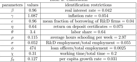
Table 3: Calibration
parameters values identi…cation restrictions 0:96 real interest rate = 0:042 1:087 in‡ation rate = 0:054
e 0:96 mean fraction of borrowing of R&D …rms = 0:04 0:64 return on deposit certi…cates = 0:075
3:4 labor share = 0:64
0:115 average hours schooling per week = 2:97 0:052 R&D employment/total employment = 0:055
474 loan o¢ cers/total employment = 0:0025 0:31 working time/total time = 0:2 f0 0:127 per capita growth rate = 0:031
.
As in King and Rebelo (1993), 20% of the total time is allocated to working. In our model, working consists of producing …nal goods, working in the innovation sector, and working for …nancial intermediaries. According to a report on occupational employment and wages by the Bureau of Labor Statistics (BLS, 2007), the fraction of loan o¢ cers to total employment in May 2005 was 0:0025.21 According to the occupational employment
statistics survey,22 the individuals employed in science and engineering occupations was
5:5% of the total workforce in May 2007. In Ramey and Francis (2009), the average hours schooling per week are 2.97, and the average hours worked per week are 21.71 (average of 1965-2005). Since we have normalized total working hours to 0.2 in the model, the corresponding model hours for schooling are 0:0274. Brown and Petersen …nd that the mean fraction of debt to total assets of young R&D …rms is 4% (Table 1, p. 700).23
Finally, a labor share of 0:64 is standard.24
As discussed further below, the key to understanding the large growth e¤ects of in‡ation is search as represented by the matching probability and the search time . The target "average hours of schooling per week", among other targets, pins down the search time . It captures the fact that a fraction of the cost of the innovation process is non-random and arises from the time spent in education or from learning-by-doing.25 It complements our
target "R&D employment to total employment", which, among other targets, pins down
21According to this report, in May 2005, 332,690 people were working as loan o¢ cers and total
employ-ment in the economy was 130,307,850. The implied ratio 0:0025 is similar to the number 0:0028 used by Dotsey and Ireland.
22Statistical Abstract of the U.S. 2009, Table 788.
23They classify a …rm as young for the …rst 15 years following the year it …rst appears in Compustat
with a stock price.
24We provide step-by-step instructions of our calibration strategy in the supplementary material. 25In our model, only potential innovators spend time in education, whereas our target "average hours of
schooling per week" corresponds to the average time spent of the entire population. Since the typical R&D employee spends more time in education than the average citizen, our target is rather low. Increasing the value of the target would result in a higher value of (see the calibration procedure in the supplementary material), and, as shown in Section 5, a higher value of generates larger growth e¤ects of in‡ation.
the matching frictions . Here, the matching friction captures the fact that the innovation process is random and that not all potential innovators can successfully contribute to a household’s increase in productivity.
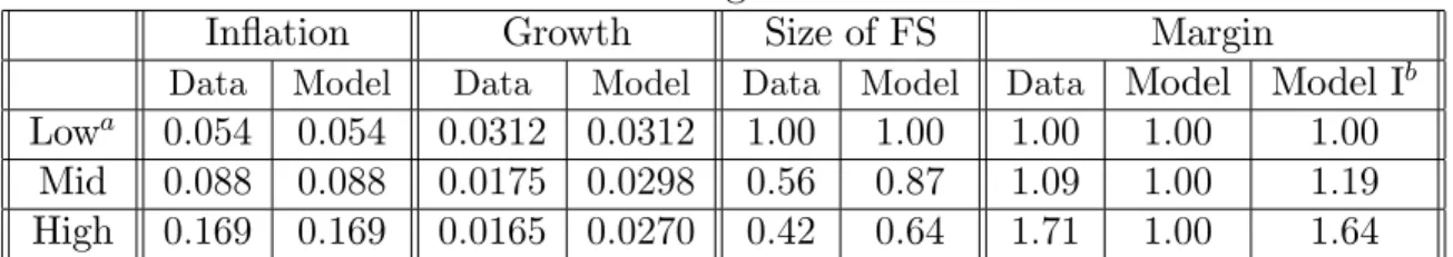
Table 4: E¤ects of in‡ation on growth and the …nancial sector In‡ation Growth Size of FS Margin
Data Model Data Model Data Model Data Model Model Ib
Lowa 0:054 0:054 0:0312 0:0312 1:00 1:00 1:00 1:00 1:00
Mid 0:088 0:088 0:0175 0:0298 0:56 0:87 1:09 1:00 1:19 High 0:169 0:169 0:0165 0:0270 0:42 0:64 1:71 1:00 1:64
aThe in‡ation rate and the per capita growth rate of the average low-in‡ation country are used as targets for the baseline calibration.bModel I is the baseline model with an intensive margin presented in Section 6.1
Table 4 compares the model’s predictions on in‡ation, the growth rate, the size of the …nancial sector (FS) and the interest margin with the data. For the average low-in‡ation country, the growth rate has the same value in the model as in the data, because it is used as a target in the calibration. We also set the in‡ation rates of mid- and high-in‡ation countries to match the data. Our model does a reasonable job in replicating the change in the size of the …nancial sector. When in‡ation increases from low to high levels, the per capita growth rate and the size of the …nancial sector fall in the model as well as in the data, although it falls more sharply in the data.
Our baseline model cannot replicate the change in the interest margin, since, from (23), the interest spread is independent of in‡ation. In Section 6.1, where we enhance the baseline model with an intensive margin (i.e., households obtain the choice of how many hours to work in a match), the interest-rate margin is increasing in in‡ation and matches the increase of the interest-rate margin observed in the data (see the column labeled Model I in Table 4).
Note that in‡ation in our model can only explain a fraction of the observed fall in per capita growth and the fall in the size of the …nancial sector. For example, in the data per capita growth in the average high-in‡ation country is about 45% lower than in the average low-in‡ation country. The model only predicts a decrease of about 13.5% (from 3.12% to 2.7%). This is not surprising, as one would expect that the two country types di¤er in many other characteristics that also a¤ect per capita growth.
4.2
Welfare analysis
We now quantify the cost of in‡ation by focusing on the balanced growth path. Denote the net rate of in‡ation as . Following the literature (e.g., Lucas, 2000, and Lagos and Wright), we measure the welfare cost of in‡ation at relative to 0 by asking how much
consumption (in percentage) agents would be willing to give up in order to change in‡ation from to 0. To express this measure formally, let be any given in‡ation rate and any
fraction. Slightly abusing an earlier notation, we write the household’s expected discounted utility under ( ; ) as:
V ( ; ) = 1 X t=1 t 1 fln ( q) + f1 k h le [ + (1 )]gg
where the quantities (q; l; k; h) take their values on the equilibrium balanced growth path at = 1. Note that q is not stationary on the balanced growth path; rather, it grows at the gross rate g. Expressing qt= q1gt 1, we can rewrite the expected utility as
V ( ; ) = 1
1 ln ( q1) + 1 ln (g) + f1 k h le [ + (1 )]g
The welfare cost of in‡ation at relative to 0 is the value of (1 )that solves V ( 0; ) =
V ( ; 1).
4.3
The growth and welfare e¤ects of in‡ation
Consider the three groups of countries that di¤er in the in‡ation rate; i.e., the countries with low in‡ation (5.4%), medium in‡ation (8.8%), and high in‡ation (16.9%). For each of these groups, Table 5 reports the key variables on the balanced growth path. Also, Table 5 reports the gains in welfare and the growth rate from moving to zero in‡ation.
As Table 5 shows, the time spent in innovation decreases signi…cantly after an increase in in‡ation. As a result, the growth rate is decreasing in in‡ation, and this negative e¤ect of in‡ation on growth is large. For the average medium-in‡ation country, reducing its in‡ation from the average (8.8%) to zero increases the long-run growth rate by 0.42 percentage points. For the average high-in‡ation country (16.9%), reducing its average in‡ation to zero increases the long-run growth rate by 0.69 percentage points. These e¤ects of in‡ation on growth fall into the range of empirical estimates obtained from cross-country studies (see the references in the Introduction). They are much larger than the growth e¤ects of in‡ation found in the literature. In Gomme, and Dotsey and Ireland, for example, reducing in‡ation to zero in a similar experiment increases growth by only 0.05 percentage points.
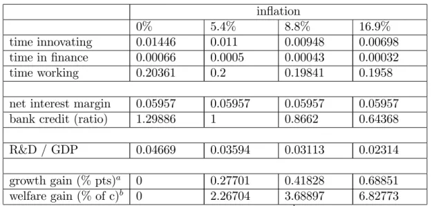
Table 5: E¤ects of in‡ation in the baseline model in‡ation 0% 5.4% 8.8% 16.9% time innovating 0.01446 0.011 0.00948 0.00698 time in …nance 0.00066 0.0005 0.00043 0.00032 time working 0.20361 0.2 0.19841 0.1958
net interest margin 0.05957 0.05957 0.05957 0.05957 bank credit (ratio) 1.29886 1 0.8662 0.64368
R&D / GDP 0.04669 0.03594 0.03113 0.02314
growth gain (% pts)a 0 0.27701 0.41828 0.68851
welfare gain (% of c)b 0 2.26704 3.68897 6.82773 a
Growth gain in percentage points from reducing the in‡ation rate to 0%.bWelfare gain as a percentage of consumption from reducing the in‡ation rate to 0%.
Higher rates of in‡ation also a¤ect the …nancial market considerably. Table 5 shows that the size of the …nancial market relative to the economy decreases signi…cantly with in‡ation, as indicated by the large reduction in the ratio of loans to GDP. For the medium-in‡ation country, the ratio of loans to GDP is only 87% of the ratio for the low-medium-in‡ation country, and for the high-in‡ation country this ratio is 64% of the ratio for the low-in‡ation country.
In‡ation has large welfare e¤ects. For the low-in‡ation country, the welfare gain from reducing in‡ation from the historical mean (5.4%) to zero is 2.3% of consumption. For the medium-in‡ation country, the welfare gain from reducing in‡ation from the historical mean (8.8%) to zero is 3.7% of consumption. For the high-in‡ation country, the corresponding welfare gain is 6.8% of consumption. These welfare e¤ects are considerably larger than the ones obtained in the literature (e.g., Dotsey and Ireland), because in‡ation has a much larger negative e¤ect on growth in our model than in the literature.
The growth e¤ects of in‡ation are large, because in‡ation reduces the members allocated to the innovation sector substantially. For example, for the average high-in‡ation country, the time innovating is less than 65% of the time of the average low-in‡ation country. This is also re‡ected by the much lower R&D/GDP ratio which is 2.31% for the average high-in‡ation country versus 3.59% for the average low-in‡ation country.26
26Note that our R&D/GDP ratio for the average low-in‡ation country is higher than the average of R&D
expenditure as a percentage of GDP for the US, which is 2.62% for 1981-2006 (Factbook 2008: Economic, Environmental and Social Statistics, OECD). The reason is that we calibrate our model to the fraction of individuals employed in science and engineering, which is 5.5%.
5
The Role of Search and Comparison with CIA
Why do we need microfoundations, and do they matter for any substantive results? These and related questions are often raised when we present a search-and-bargaining framework in monetary economics. Since all of the papers mentioned in the introduction use cash-in-advance, henceforth CIA, models, we obviously do not need a search-and-bargaining model to study the e¤ects of in‡ation and …nancial intermediation on growth. However, as emphasized by Berentsen et al. (2011) and Shi (1998), the important issue is not one of need, but whether it matters for the results whether one uses microfoundations or a reduced-form approach.
To discuss this issue and to gain further insights into the mechanics of the baseline model, we investigate the role of search, as represented by the parameters and . Further-more, we construct and calibrate a prototypical CIA-model with a frictionless competitive innovation market, and compare it to the search model.
5.1
The role of search
The key for understanding the large e¤ects of in‡ation on growth and welfare is search. Search is represented by the parameters and , where re‡ects the matching frictions in the innovation market, and , the time used searching. To highlight the importance of search for our results, we present and discuss the growth and welfare e¤ects for various exogenous values of or .
The e¤ects of the matching probability In Table 6, we explore the key e¤ects of the matching friction .27 Results for the following values of are presented: = 0:052,
which corresponds to the calibrated value of the baseline model; = 0:026, which is one half of that amount; = 0:5; and = 1. The value = 0:5 corresponds to the case where all potential innovators are matched; one half of them as buyers and the other half as sellers of innovation time. For = 1, the interpretation of the matching process is di¤erent.28 In this case, all potential innovators that enter the innovation market are randomly matched to one other household, which hires them as innovators. Recall that there is still search time since > 0, meaning that a potential innovator in a match can work only 1 hours.
27In the following, we only present the calibration results. The derivation of each model and details of
the calibration are available as supplementary material. Except for the exogenous choice of , all other elements of these models are equivalent to the baseline model described in Section 4. For each exogenous value of in Table 6, we remove the target "fraction of loan o¢ cers to total employment" (see Table 3) and recalibrate the model. Instead of removing this target, we have also removed the target "mean fraction of borrowing of R&D …rms". The results are essentially the same.
28We present this case because it is closely related to the natural cash-in-advance model presented below.
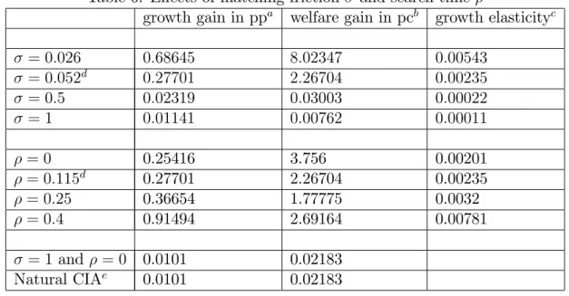
Table 6: E¤ects of matching friction and search time
growth gain in ppa welfare gain in pcb growth elasticityc
= 0:026 0:68645 8:02347 0:00543 = 0:052d 0:27701 2:26704 0:00235 = 0:5 0:02319 0:03003 0:00022 = 1 0:01141 0:00762 0:00011 = 0 0.25416 3.756 0.00201 = 0:115d 0.27701 2.26704 0.00235 = 0:25 0.36654 1.77775 0.0032 = 0:4 0.91494 2.69164 0.00781 = 1 and = 0 0.0101 0.02183 Natural CIAe 0.0101 0.02183 a
Growth gain in percentage points from reducing the in‡ation rate to 0%. bWelfare gain as a percentage of consumption from reducing the in‡ation rate to 0%. cElasticity of the growth rate with respect to the net in‡ation rate.dCorresponds to the baseline calibration. eE¤ects of in‡ation in the natural model of cash-in-advance in the innovation market.
The key e¤ects of the matching parameter are displayed in the …rst two rows of Table 6. All values in Table 6 are calculated for the average low-in‡ation country. First, in comparison with the baseline calibration ( = 0:052), the growth e¤ects of in‡ation are much smaller for = 0:5 and = 1, and strikingly larger for = 0:026. For example, for the average low-in‡ation country, reducing in‡ation from the historical mean (5.4%) to 0% increases the long-run growth rate by 0:011 percentage points for = 1, and by 0:686 percentage points when = 0:026. Second, the welfare cost of in‡ation are much smaller for high values of . For example, for the average low-in‡ation country, the welfare gain from reducing in‡ation from the historical mean to zero is 8% of consumption for
= 0:026, and only 0:0076% when = 1.
How does in‡ation a¤ect growth? To understand the mechanism requires us to study the …rst-order condition for l; i.e., equation (25), which, using (2), can be written as follows
f (i)
elR [1 + f (i)] = [ + (r`+ )(1 )] (27) The left-hand side of (27) is the expected bene…t of allocating an additional potential innovator to the innovation market. The right-hand side is the expected cost of doing so, which depends on the borrowing cost r`. Since, from (27), the measure of innovators
in‡ation. Therefore, the growth rate 1 + f (i) is decreasing in in‡ation.29 The extent to
which in‡ation a¤ects the growth rate depends on , since a¤ects the elasticity of l with respect to in‡ation. In Table 6 we present the elasticities of l and g with respect to in‡ation for various values of . They are decreasing in , meaning that the measure of innovators and hence the real growth rate becomes less sensitive to changes in in‡ation as
increases.30
Why are the e¤ects of in‡ation on growth sensitive to changes in the matching prob-ability ? To understand how these elasticities depend on , one needs to understand the costs of holding money. In the baseline model, all money is allocated to the potential innovators. Those that have no access to the innovation market can deposit their money and earn interest rd, which partially compensates for the in‡ation tax. Those that have
access to the market earn no interest, rather they borrow additional money at rate r`. The
bene…t of holding money (i.e., the opportunity to spend it) only arises with probability , since only with this probability does a potential innovator meet a seller from some other household, who has the needed skills.
A small , thus, means that a large fraction of the money holdings are not spent in a period. That is, while the entire money holdings are subject to the in‡ation tax, only a small amount of it is spent and generates utility to the household. Consequently, the household reacts very sensitively to a change in the cost of holding money. When in‡ation increases, the household attempts to reduce its exposure to the in‡ation tax by reducing the number of members allocated to the innovation sector. With a larger , the cost of holding money remains the same, but now the probability of spending it increases, and so the bene…t-cost ratio improves. Consequently, the household reacts less sensitively to changes in the cost of holding money.
A small captures the empirical evidence on the use of cash for R&D activities (see our discussion in the introduction): …rms with large R&D activities hold large amounts of cash. Naturally, then, the innovation sector reacts very sensitively to the in‡ation tax.
The e¤ects of the search time The growth e¤ects of are qualitatively similar to the growth e¤ects of . For example, for the average low-in‡ation country, reducing in‡ation from the historical mean (5.4%) to 0% increases the long-run growth rate by 0:27701 percentage points for = 0:115, and by 0:25416 percentage points for = 0 (see Table 6). For = 0:4, the growth loss is substantially larger, namely, 0:91494 percentage points.31
29From (22) and (23), r
` is increasing in the gross growth rate of the money supply ; i.e., drd` = 1.
Since and satisfy = (1 + )g and g is decreasing in , and are positively related.
30Table 6 presents the elasticities for di¤erent values of , where for each value we recalibrate all other
parameters using the same targets as for the baseline calibration. Alternatively, one can calculate these elasticities by keeping all other parameters constant. In this case, we can get an explicit expression for the elasticity of g with respect to . One can show analytically that this elasticity is decreasing in .
31For each exogenous value of in Table 6, we remove the target "average hours schooling per week"
and recalibrate the model. The details of the calibration are available as supplementary material. Except for the exogenous choice of , all other elements are equivalent to the baseline model described in Section 4. Notice that we cannot increase above 0:45, since the calibration would yield a convex innovation function; i.e., > 1.
Table 6 also shows the elasticity of the growth rate with respect to the net in‡ation rate. For example, for the average-low in‡ation country, increasing the in‡ation rate by 1%; i.e., from 5:4% to 5:454%, reduces the growth rate by 0:00201% when = 0 and by 0:00235% when = 0:115. The elasticity of the growth rate with respect to in‡ation is increasing in
: It is almost four times higher for = 0:4 (0:00781) than for = 0 (0:00201).
Note that the welfare cost of in‡ation is lower in the calibrated model with = 0:25 than in the calibrated model with = 0. This can be explained as follows. When in‡ation is reduced to zero, l increases and, thus, the growth rate increases. However, the extent to which the increase in the growth rate improves welfare depends partly on how the loss in leisure time by innovators is valued by the household. A high value of exacerbates the loss in leisure time since innovators must spend more time searching.32 As a result, the
welfare gain of reducing in‡ation is not necessarily higher for a higher value of .
The case = 0 and = 1 Finally, we report the e¤ects of in‡ation when there are no search costs, = 0, and no matching frictions, = 1. This case is of interest because it is closely related to the natural model of cash-in-advance presented below. With = 0 and = 1, reducing in‡ation from 5:4% to 0% increases the growth rate by 0:0101 percentage points, and the welfare gain in terms of consumption is 0:02183%. Reducing in‡ation from 8:8% to 0% increases the growth rate by 0:01614 percentage points, and the welfare gain in terms of consumption is 0:04015%. Finally, reducing in‡ation from 16:9% increases the growth rate by 0:02985 percentage points, and the welfare gain in terms of consumption is 0:09551%.33
5.2
A natural model of cash-in-advance in the innovation market
Consider the following version of the baseline model with no search and a CIA-constraint in the innovation market. The household chooses ls innovators who are employed by other
households at the competitive wage p. The household also hires lb innovators from other
households. The representative household’s problem is34
V (a; m) = max
z fu [q (h; a)] + (1 k h ls) + V (a+1; m+1)g
32This e¤ect is not compensated by the change in the value of , since, given the calibration procedure,
the value of remains unchanged when is modi…ed (see the supplementary material). In contrast, when is exogenously …xed, the calibrated value of depends on the value of , since adjusts to match the target on average schooling hours.
33To obtain these values, we have eliminated the targets "fraction of loan o¢ cers to total employment"
and "average hours schooling per week." The derivation of the model and its calibration is presented in the supplementary material.
34
subject to the following constraints:
bd (1 e) m
plb em + b`
a+1 = a + af (lb)
m+1 m = pls plb+ rdbd r`b`+ wk + T:
The household enters the period with m units of money. To generate a role for …nancial intermediation, we assume that he can only use the fraction e to purchase innovation goods. The fraction 1 e is illiquid. The household deposits the illiquid funds in the …nancial sector to earn interest rate rd. Financial intermediaries, then, lend it out to other
households at interest rate r`.
The growth and welfare e¤ects of in‡ation are very small, comparable in magnitude to the ones reported in previous CIA-models mentioned in the Introduction. Furthermore, they are exactly equal to the losses presented above for = 1and = 0 (see Table 6). This should come as no surprise, as any natural CIA-model with competitive markets ignores search by de…nition.
6
Extensions
In this section, we study two extensions of the baseline model. First, we add an intensive margin by letting the household choose how much time a buyer acquires from the seller in a match. The main e¤ect of the intensive margin is that the model now matches the increase in the interest rate margin that we observe in the data. The growth and welfare e¤ects of in‡ation are slightly larger than the ones of the baseline model. Second, one might conjecture that our large growth and welfare e¤ects are a result of our assumption that money is only needed in the innovation sector. Here, we show that this is not the case. Rather, if money is also needed for transactions in the goods market, the e¤ects of in‡ation on growth are larger than in the baseline model.
6.1
The roles of the intensive and extensive margins
In this section, we add an intensive margin to the innovation sector by letting the house-holds choose how much innovation time a member buys if he is matched to a seller, denoted as y. Furthermore, we assume that the contribution of y units of time to the innovation process is c (y) where c (y) = c0y , with 0 < < 1 and c0 > 0. These assumptions also
involve replacing 1 by Y in (9), because the quantity Y is chosen by the household’s trading partners.
For ease of comparison, we state the representative household’s problem:35
V (a; m) = max
z fu [q (h; a)] + f1 k h el ( + Y )g + V (a+1; m+1)g
35Here, the decision variables of the household are z [q; l; k; h; x; y; b