Prescribed energy connecting orbits for gradient systems
34
0
0
Texte intégral
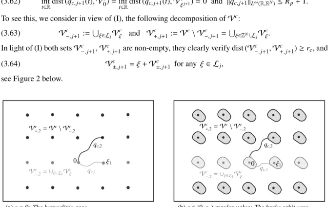
Figure
Documents relatifs