Three decades of trace element sediment contamination: The mining of governmental databases and the need to address hidden sources for clean and healthy seas

Environment International 149 (2021) 106362

Available online 3 February 2021

0160-4120/© 2020 The Authors. Published by Elsevier Ltd. This is an open access article under the CC BY license (http://creativecommons.org/licenses/by/4.0/).

Three decades of trace element sediment contamination: The mining of

governmental databases and the need to address hidden sources for clean

and healthy seas

Jonathan Richir

_{, Simon Bray}

_{, Tom McAleese}

_{, Gordon J. Watson}

b_{Chemical Oceanography Unit, FOCUS, University of Li`ege, Li`ege, Belgium} c_{Laboratory of Oceanology, FOCUS, University of Li`ege, Li`ege, Belgium} d_{AQASS Ltd, Hound Road, Southampton SO31 5QA, UK}

e_{School of Biological Sciences, Life Sciences Building 85, University of Southampton, SO17 1BJ, UK}

A R T I C L E I N F O Handling Editor: Frederic Coulon Keywords: Sediment Metal Metalloid Benthic Antifouling Shipping Eutrophication A B S T R A C T

Trace elements (TEs) frequently contaminate coastal marine sediments with many included in priority chemical lists or control legislation. These, improved waste treatment and increased recycling have fostered the belief that TE pollution is declining. Nevertheless, there is a paucity of long-term robust datasets to support this confidence. By mining UK datasets (100s of sites, 31 years), we assess sediment concentrations of arsenic (As), cadmium (Cd), chromium (Cr), copper (Cu), iron (Fe), mercury (Hg), nickel (Ni), lead (Pb) and zinc (Zn) and use indices (PI [Pollution], TEPI [Trace Element Pollution] and Igeo [Geoaccumulation]) to assess TE pollution evolution. PI and TEPI show reductions of overall TE pollution in the 1980s then incremental improvements followed by a distinct increase (2010–13). Zn, As and Pb Igeo scores show low pollution, whilst Cd and Hg are moderate, but with all remaining temporally stable. Igeo scores are low for Ni, Fe and Cr, but increasing for Ni and Fe. A moderate pollution Igeo score for Cu has also steadily increased since the mid-1990s. Increasing site trends are not universal and, conversely, minimal temporal change masks some site-specific increases and decreases. To capture this variability we strongly advocate embedding sufficient sentinel sites within observation networks. Decreasing sediment pollution levels (e.g. Pb and Hg) have been achieved, but stabilizing Igeo and recently increasing TEPI and PI scores require continued global vigilance. Increasing Ni and Fe Igeo scores necessitate source identifica-tion, but this is a priority for Cu. Local, regional and world analyses indicate substantial ‘hidden’ inputs from anti-fouling paints (Cu, Zn), ship scrubbers (Cu, Zn, Ni) and sacrificial anodes (Zn) that are also predicted to increase markedly. Accurate TE input assessments and targeted legislation are, therefore, urgently required, especially in the context of rapid blue economic growth (e.g. shipping).

1. Introduction

Coastal regions contain some of the most ecologically productive habitats and are critical for their goods and services (Hassan et al., 2005; Watson et al., 2020). Yet, coastal sediments are often heavily contami-nated by metals and metalloids from human activities, leading to sediment accumulation (Bryan and Langston, 1992) and human health risks from bioaccumulation (e.g. Liu et al., 2020). These trace elements (TEs) are also some of the most significant aquatic pollutants with Johnson et al. (2017)

placing 10 in the top 20 most toxic substances. To reduce concentrations and toxicological effects and to achieve healthy and clean oceans many TEs are included in priority chemical lists (e.g. US EPA, 2015) or other legislation (e.g. EU, 2000). In addition, governments have expected that technological advances in manufacturing and improved waste manage-ment and recycling will also reduce inputs. This has fostered a belief in some that TE contamination is generally resolved (i.e. a legacy); com-pounded by attention being focused elsewhere (e.g. microplastics).

Biomarker programmes such as ‘Mussel Watch’ can provide evidence * Corresponding authors at: Institute of Marine Sciences, School of Biological Sciences, University of Portsmouth, Ferry Road, Portsmouth PO4 9LY, UK (J. Richir and G.J. Watson).

E-mail addresses: [email protected] (J. Richir), [email protected] (G.J. Watson). 1 _{Authors equally contributed to this study.}

Contents lists available at ScienceDirect

Environment International

https://doi.org/10.1016/j.envint.2020.106362

Environment International 149 (2021) 106362 of TE temporal decline, yet they have significant biological limitations

(see Farrington et al., 2016). Selected bivalves are also ‘disconnected’ from benthic sediment habitats, for example, mussels attach to hard substrates in the water column (Gosling, 1992). Bivalves play a signifi-cant role in assessing contamination (see Beyer et al., 2017), but their utility lacks sediment-specific habitat relevance. Without a recognised mussel-equivalent sentinel infaunal species, research has focused on sediment matrix concentrations. One approach is to reconstruct histor-ical contamination using sediment cores (e.g. Kang et al., 2018). How-ever, frequent human disturbance disrupts the profile; limiting relevance to areas of minimal anthropogenic activity. Long term data-sets that have been analysed are very locally focused (i.e. within one estuary) and/or have a limited sampling timescale (e.g. Traven et al., 2015; Ribeiro et al., 2018). Even those at the trans-national level are also spatially and temporally limited. For example, OSPAR (2019a) only uses the Marine Environment Monitoring and Assessment National (MERMAN) database (see below), preventing potential comparison and augmentation with examples from regional scale inshore and coastal areas. Thus globally, there is an urgent need for assessments over appropriate spatial (i.e. 1000s km of coastline and open ocean) and temporal (multiple decades) scales to confirm TE concentration re-ductions and, therefore, that the ecological health of these systems is improving.

UK coastal and marine monitoring data are held in two key public repositories: a) the Environment Agency (EA) and b) the MERMAN database managed by the British Oceanographic Data Centre (BODC) under the Clean Safe Seas Environmental Monitoring Programme (CSEMP) (Cefas, 2012). From these we generated a merged EA- MERMAN database focused on the Channel, southern North and Celtic Seas ensuring we reflect the global spectrum of contamination levels (e. g. Bryan and Langston, 1992; Haynes et al., 1995; Caplat et al., 2005; Naidu et al., 2012; Pan and Wang, 2012; Qian et al., 2015). This area also contains current and historical examples of nearly all direct anthropogenic TE inputs and key atmospheric sources (Rainbow, 2018; OSPAR, 2019a,b). By mining these data sources through our merged dataset, we first assess the evolution of sediment contamination for nine TEs (As, Cd, Cr, Cu, Fe, Pb, Hg, Ni and Zn) across multiple sites and decades. Our subsequent application of pollution indices at a broad spatial scale and over an extended period is pertinent to TE persistence, aligns with national and international legislative developments and in-corporates decadal technological changes.

Whilst the inputs of contaminants from direct, riverine and atmo-spheric anthropogenic sources have been regularly estimated, e.g. see OSPAR (2019b,c) and Richmond et al. (2020) for the UK; recently Tornero and Hanke (2016) identified sea-based sources as also potentially signif-icant contributors. From the eight sources stated we selected shipping due to its prominence in the Channel region. In addition, supporting data for shipping would likely be available to calculate input estimates. Thus, our final aim is to quantify TE inputs from three fundamental, but rarely studied components (termed ‘hidden’ here), of shipping activity: a) anti-fouling coatings, b) ship exhaust cleaning systems (termed scrubbers), and c) sacrificial hull anodes at local, national and global spatial scales and then to predict inputs for 2040. Combined, these data deliver critical in-formation for evaluating the current policies for some of the most toxic chemicals delivered to marine benthic systems. Data provide a road map for identifying best practice for using existing databases for contamination studies. Outputs will also be key for updating legislative frameworks for achieving clean and healthy seas now, but most importantly, in the future as global blue economic investment (with shipping having a pivotal role) is predicted to expand rapidly (OECD, 2016).

2. Material and methods 2.1. Data mining

Upon request the EA provided both inland and marine data for

sediment and non-sediment samples for South and South West English regions. To obtain data from only transitional, estuarine and coastline waters, georeferenced sites were mapped (Google Earth, Google LLC). An iterative process was required for quality assessment including geographic locations and sample material codes etc. The BODC dataset (from 1999) required less pre-processing with georeferenced MERMAN sites mapped. The two datasets were merged and then standardized (e.g. concentration units, duplicated sites). Our resulting EA-MERMAN database consists of 45,962 data points (334 sites) for 29 chemicals over 31 years (1983–2013). We selected the nine most monitored TEs, together representing 87% of data (320 sites). Finally, to remove outliers (i.e. samples with extremely high values) all TE values higher than or equal to 99.85 quantile were removed (approximately seven data points per TE).

2.2. General sediment sample processing

Sediment samples collected for the MERMAN database were ac-quired and processed following guidelines (Cefas, 2012). Briefly, sedi-ment samples were sieved (wet or dry) and the <63 μm fraction retained

for - usually - total digestion (td) using hydrofluoric acid (HF). The analytical technique chosen is not mandatory, but most laboratories now use Inductively Coupled Plasma Mass Spectrometry (ICP-MS) for TE determination; Hg can be determined by cold vapour atomic absorption spectrometry or atomic fluorescence. The protocol for samples collected by the EA has evolved since the 1980s with the Cefas (2012) processes applicable, but to some data only (including coastal sediment data collected under the protocols, stored in both databases). EA sediment samples were formerly wet sieved and the <90 μm fraction retained, but this was changed to retention of the <63 μm fraction in the 1990s. To

focus on TEs considered as biologically-available, extraction used strong acid digestion (sad) with hot HNO3 or aqua regia. When sediments were digested using HF, they were distinguishable in the EA database. HF, unlike hot HNO3/aqua regia, dissolves TEs bound to silicate structures. However, we have considered hot HNO3/aqua regia and HF digestions equivalent for Cu, Zn, As, Cd, Hg, Ni and Pb since those TEs are a small part of the sediment matrix; confirmed by comparing extraction effi-ciencies (Cook et al., 1997; Hall, 2017). For Fe and Cr, differences in sediment extraction efficiencies were > 10%, therefore, data from each extraction procedure were analysed separately. Our quality assurance processes ensured there was no step-change effect for changeover of analytical technique e.g. flame atomic absorption to ICP-MS (most lab-oratories); Hg would be analyzed with cold vapour technique (EA, pers. comm.). TE concentrations are given on a dry weight basis (mg kg−1_). Median detection limits (DL, in mg kgdw−1_{) were 0.1 for Cd, Cr (sad) and} Hg, 1 for Cu, 2 for As, 3 for Fe (sad), 5 for Ni and Zn and 8 for Pb. For TE concentrations below the analytical procedure DL, we used half the DL values (US EPA, 1991).

2.3. Sediment quality guidelines (SQGs) and background levels

TE concentrations were compared to SQGs. Canadian SQGs consist of Interim Marine Sediment Quality Guidelines/Threshold Effect Levels (ISQG/TEL), thereafter called TEL and Probable Effect Levels (PEL). Below the TEL, adverse effects on the biota rarely occur; between the TEL and the PEL, adverse effects on the biota may occasionally occur; above the PEL, adverse effects on biota are frequent (CCME, 2001; Simpson et al., 2013). Although Hübner et al. (2009) stated that TEL/ PEL-based SQGs are appropriate assessment criteria for contaminants in sediment with a proven scientific basis, Cefas (2012) considers as assessment criteria the Effects Range Low (ERL, developed by the US EPA [1991]) and the Background Assessment Concentrations (BAC) developed within the OSPAR Commission framework, where concen-trations below the ERL rarely cause adverse effects in marine organisms and concentrations below the BAC are said to be near background.

Sediment contamination assessments require determination of TE J. Richir et al.

background concentrations (B) for uncontaminated sediments (Brady et al., 2015; Birch, 2017). Usually historical data are not available, hence a non-contaminated analogue is needed: unpolluted reference sites (e.g. Brady et al., 2015); crustal composition (e.g. Brady et al., 2015) or sedimentary rock composition (e.g. Dung et al., 2013). How-ever, when the data represent a comprehensive cross section of a large region, B can also be defined as equal to a given dataset quantile. For example, Rainbow et al. (2011) calculated metal B values as equal to the 33rd percentile values of their concentration data and defined B as “typical” of the least disturbed areas in a region. Applying this here meant that most TEs were close to or above TEL values (S1 Table 1). Except in areas with naturally elevated background concentrations, baseline levels should not lead to any (or very little) adverse biological levels. Therefore, we have redefined B as the 20th percentile values of the concentration data, resulting in the B for As remaining slightly above the TEL, whilst all other TEs were below (SI Table 1).

2.4. Sediment quality indices

Among multiple sediment quality indices that calculate contamina-tion, the use of the Contamination Factor (CF) and related 7-level Geoaccumulation Index (Igeo) pollution scale are considered the preferred single-element indices (Brady et al., 2015). The Igeo pollution scale classifies sediments from unpolluted to very strongly polluted (Müller 1986). Igeo scale levels correspond to given CF values (Igeo = log2(CF/1.5)). The CF of a TE n is the ratio between its concentration in the sediment Cn and its natural background concentration Bn (CF = Cn/ Bn) (Tomlinson et al., 1980) and the arbitrary 1.5 factor minimizes the impact of lithogenic enrichment and enrichment caused by sediment inputs from several sources. The relationship between CF values and Igeo scale levels is from Legorburu et al. (2013), but using a blue-red colour scale. The Nemerov Pollution Index (PI) (Nemerow, 1991) is the most comprehensive method for overall sediment quality and has been increasingly used in recent years (see Brady et al., 2015). PI uses the average of CF (CFaverage) of a suite of TEs focusing on the impact of contamination of one TE by using the maximum CF (CFmax) (PI=((CFa-verage2 + CFmax2 )/2)1/2). The 5-level sediment quality scale classifies sediments from unpolluted (PI < 0.7) to severely polluted (PI > 3) (Brady et al., 2015; Qingjie et al., 2008). As the PI is weighted by the effect of a single TE and values are also strongly dependent on Bs, it may lead to an overestimation of the overall TE pollution status. A comple-mentary index to the PI, is the Trace Element Pollution Index (TEPI) of Richir and Gobert (2014). TEPI does not rely on pre-determined back-ground concentrations and does not give higher importance to a more polluting TE. TEPI is the weighted product of mean normalized (Moreda- Pi˜neiro et al., 2001) TE concentrations Cf of the n TE under study (TEPI =(Cf1 * Cf2 … Cfn)1/n). This weighted index also enables reliable com-parison of TE pollution levels even if the list of monitored TEs used differ (Richir and Gobert, 2014). The 5-level environmental quality scale of Richir et al. (2015) applied to TEPI values relies on the quantile method and classifies sediments from Very Low Contamination Level (VLCL) to Very High Contamination Level (VHCL). To utilize a more complete matrix for the PI and TEPI, site TE concentrations were averaged every five years (seven for 1983–1989, four for 2010–2013). The PI and TEPI were then calculated for all sites that, for those periods, had a minimum of six mean concentrations for the nine TEs monitored.

2.5. Input estimates (antifouling paints, scrubbers and anodes)

The Solent separates the Isle of Wight from mainland England and is contained within the Channel; the water body between France and En-gland and a component of the ecoregions of the Greater North Sea and Celtic Seas (ICES, 2020). Both the Channel and Solent are protected by many conservation designations, but also host several international commercial ports and high levels of recreational/commercial boating activity. To count the number of vessels in the Solent on any given day

satellite images (Google Earth, 2019) were analysed. A 2,304 km2 _grid (256 cells) overlaid on the map defined the Solent and within each cell all vessels below high water line (includes those located on intertidal habitats, but not dry dock) were counted (see S2 Table 1). To calculate the proportions of each vessel type, AIS (Automatic Identification Sys-tems) tracking software (https://www.vesselfinder.com/) was used once a day for 10 days with vessel details extracted (S2 Table 2). These data were then used to calculate underwater surface area (UWSA) using specific vessel-type formulas (S2 Table 3). Daily AIS count data (signals that were not vessels or unspecified were removed) were also purchased from MarineTraffic for a 65,000 km2 region defined as the Channel (S2 Table 1). Recreational vessel numbers (USA: Boating Industry Market, and ICOMIA report) were included as was the global fleet of merchant vessels (S2 Table 1). Mean, maximum and minimum predictions for changes in vessel numbers by 2040 (USA recreational and global mer-chant fleets) were calculated using the corresponding mean, maximum and minimum values calculated for the percentage increase/decrease between consecutive years in the number of vessels for the source data. These were then applied to each year up until 2040.

To estimate inputs from different sources and into different areas we have provided realistic (means), maximum and minimum scenarios. Anti-fouling (AF) data (e.g. Cu and Zn based anti-fouling paint use, release rates etc.) were combined with the Underwater Wetted Surface Area (UWSA) and vessel numbers (data source details given in S2 Tables 1–4) to calculate AF paint Cu and Zn inputs (example calculations pro-vided in S2). For scrubber inputs we used Cu, Zn and Ni discharge rates and then used the mean, maximum and minimum calculated values for the proportion of vessels using scrubbers, combining scrubber use, type (open v. hybrid/closed), wastewater discharge rates (assuming a 10 mW engine) and vessel count data (S2 Tables 1, 5). The number of anodes required to protect a merchant vessel was calculated based on a hull’s current requirement combined with the proportion of each vessel type and the number of vessels in an area (S2 Tables 1, 2, 6), whilst mean Zn release rates generated the equivalent for recreational vessels (S2 Tables 1, 2, 6).

2.6. Statistical analysis

The trend analyses of TE Igeo values were performed using the five- year moving average method. TE data for sites monitored for a mini-mum six years were analysed using median regression with boot-strapped standard errors, with p-value threshold of 0.05 in agreement with OSPAR (2019a) excluding sites for Cd (21 sites), Hg (12 sites) and Cr (1 site) where ≥ 25% of data were below DL. Quantile (including median) regression is robust to outliers; avoids parametric distribution assumptions; estimates rates of change in all parts of the response var-iable distribution and is invariant to monotonic transformations (Cade and Noon, 2003; Koenker and Bassett, 1978). Data processing and analysis were performed with R (R Core Team, 2020) in RStudio (RStudio Team, 2019), using R’s base function and additional functions mainly from packages: dplyr (Wickham et al., 2020), tidyr (Wickham and Henry, 2020), stringr (Wickham, 2019), pracma (Borchers, 2019), matrixStats (Bengtsson, 2020) and quantreg (Koenker, 2019). 3. Results and discussion

3.1. EA-MERMAN Database: A globally relevant resource

Our combined EA-MERMAN database is a searchable source of sediment contamination data covering approximately 80,000 km2 _of ocean and nearly 2,000 km of coastline over 31 years. Of the 39,906 data points for the nine TEs, 96% correspond to coastal sites (i.e. sites in transitional, estuarine and coastline waters), 4% as open sea sites (distant/remote from coastline). A mean of 4,434 ± 607 SD observations per TE (both digestion procedures considered together for Fe and Cr) indicates a similar TE monitoring effort, but effort over time was highly

Environment International 149 (2021) 106362 variable for sites. For example, 49 sites were monitored for at least eight

years; in contrast, 230 sites were surveyed only twice or less (median values, all TEs considered). Infrequent sampling dominates the open sea sites (97% were sampled once, usually in 2008, 2009 or 2012). Moni-toring effort also varies more broadly across the decades; effort was relatively low from 1983 to 1993, then increased substantially remain-ing high until the 2010s. It is not surprisremain-ing that samplremain-ing effort varies spatially and temporally and differs by TE. Evolving legislative and scientific drivers and improvements in analysis methods are all impor-tant. However, to harness the power of long term databases to address critical local, regional and global 21st century environmental problems, monitoring regimes must be coordinated and supported beyond the term of individual governments and funding (Hawkins et al., 2013). We, therefore, strongly advocate that sufficient sentinel sites representing key regional locations/habitats and levels of anthropogenic activity are (or continue to be) regularly monitored.

3.2. TE concentrations

Given the extensive temporal and spatial coverage of the dataset, variability in TE concentrations is, not surprisingly, considerable (see S1 Table 1). For example, concentrations of Cu ranged from 0.4 to 4,007 mg kg−1_{. TE median concentrations were maximal for Fe (25,366 or} 30,900 mg kg−1 _{depending on sad or td, respectively), minimal for Hg} (0.18 mg kg−1_{) and decrease in the following order: Fe > Zn > Cr > Pb} >Cu > Ni > As > Cd > Hg (S1 Table 1). The fraction of samples below the DL was <1% for all TEs except Hg (12.2%) and Cd (23.5%). This confirms that, despite the technological changes in detection methods over the sampling period, the full concentration range of the vast ma-jority of TEs was measured. Concentrations of TEs from some sites and sampling times were extremely high (e.g. 54.2 mg kg−1 _{for Cd in a site} contaminated by abandoned metal mines [Yim, 1976], see S1 Table 1). TE concentrations are globally comparable, with mining or point source pollution usually responsible for extremely high values (Bryan and Langston, 1992; Haynes et al., 1995; Caplat et al., 2005; Naidu et al., 2012; Pan and Wang, 2012; Qian et al., 2015). However, the

contribution of any outlier that remained after applying the filtering process, is also down weighted due to database size, pollution indices (except the PI) and statistical methods used.

The percentage of samples from the full dataset within each Igeo and CF category presented in Table 1 identify three clear TE groupings. Cr, Fe and Ni show no to moderate pollution levels for the vast majority of samples (percentage of samples below Igeo 1–2 and CF 3–6 scores: Cr: 93–97%; Fe: 99%; Ni: 90%). Zn, Pb and As have a much higher pro-portion of samples that are moderately or strongly polluted (percentage of samples Igeo 1–4 and CF 3–24 scores: As: 15%; Pb: 27.9%; Zn: 24.7%). Finally, 22, 36 and 45% of samples show moderate-strong to very strong pollution levels for Cu, Hg and Cd, respectively. These data reflect the diverse TE-specific enrichment and elevated concentrations in sites impacted by anthropogenic processes over a 31-year period (and older industrial inputs for undisturbed sediments) across the region (see Brady et al., 2015; Qian et al., 2015).

3.3. Temporal evolution of global pollution

The TEPI and the PI capture a global measure of TE contamination with the results (medians, quartiles, ranges and outliers) presented in Fig. 1. During the 1983–89 period TEPI median values were in the High Contamination Level class, but subsequently reduced to the Medium Contamination Level. Over the next 25 years it remained within this class limit, but with a continuous improvement as well as a reduction in variability as indicated by the reducing quartile ranges. A very similar pattern for the PI is also evident, but with median values always above, sometimes close (2005–09 period) to the severe pollution threshold. Although the 1980s reduction may have been due to lower sampling effort, subsequent incremental improvements are to be commended. However, the region is still severely polluted (PI) or moderately contaminated (TEPI) depending on the index used. (The difference in severity is the due the preponderance given to the TE with the highest CF and the definition of TE background concentrations for the PI). The overall slowly decreasing trends of PI and TEPI data confirm elevated TEs in sediments across a multi-decadal time scale despite substantial

Table 1

Percentage of sites (all sites together, coastal sites or open sea sites) monitored on a yearly basis, integrated over the full 31-year monitoring time series, distributed among the seven pollution levels of the Geoaccumulation Index scale, for each studied TE. Digestion techniques: strong acid digestion (sad) or total digestion (td) are specified and considered separately for Cr and Fe.

Igeo =Geoaccumulation Index. CF = Contamination Factor.

Number in brackets = number of sites monitored, on a yearly basis, over the 31-year time series.

Fig. 1. Boxplots (median [bold line]; Q1 and Q3 [boxes], ranges [whiskers] and outliers [open circles]) of Nemerov Pollution (PI) and Trace Element Pollution (TEPI) indices (PI boxplots are double square root transformed). Indices were generated with sites monitored for minimum six trace elements out of nine per four to seven-year periods. Pollution scales for TEPI classify sedi-ments (see Richir et al., 2015 for details) ac-cording to 5 levels: blue: very low contamination level (VLCL, data below the 1st quartile mean); green: low contamination level (LCL, data be-tween the 1st and 2nd quartile means); yellow: medium contamination level (MCL, data between the 2nd and 3rd quartile means); orange: high contamination level (HCL, data between the 3rd and 4th quartile means); red: very high contam-ination level (VHCL, data above the 4th quartile mean). For the PI (see Brady et al., 2015): blue: unpolluted (PI < 0.7); green: slightly polluted (0.7 < PI < 1); yellow: moderately polluted (1 < PI < 2); orange: heavily polluted (2 < PI < 3); red: severely polluted (PI > 3). (For interpreta-tion of the references to colour in this figure legend, the reader is referred to the web version of this article.)

Fig. 2. TE sediment contamination evolution using the 7-level Geoaccumulation Index (Igeo) pollution scale classifying sediment from unpolluted (blue) to very strongly polluted (red) (see Table 1 and Müller, 1986 for details). Dark squares: annual medians; dark circles: annual means; light grey crosses: site-specific annual means; full black lines: 5-year moving averages. Digestion techniques: strong acid digestion (sad) or total digestion (td) are specified and considered separately for Cr and Fe. (For interpretation of the references to colour in this figure legend, the reader is referred to the web version of this article.)

Environment International 149 (2021) 106362 investment in legislation controlling anthropogenic inputs,

improve-ments in technology, changes in regional manufacturing effort and increased recycling. However, what is most concerning is that for 2010–13 there was a distinct increase in indices’ median scores and associated quartile range for PI. Recalculating the TEPI excluding Ni and Cu (which from Fig. 2 show increasing Igeo values), puts the median TEPI and PI values for 2010–2013 closer to that of 2000–2004 (difference between periods decreases by 47% for TEPI and 19% for PI). It, there-fore, seems probable that changes in Ni and Cu make an important contribution to the recent increased TEPI and PI scores for this period (S1 Figs. 1 and 2). Considering sites are located within a region of mature (often declining) industry and where some of the most comprehensive legislation for contaminants has been enacted, it is highly likely that the trends identified here are, at best, replicated across equivalent areas, or at worst much more dramatic. Our data highlight the urgent need to assess current regional inputs of all TEs into our seas, thus confirming if the national and international legislation is effective for those that are currently priority pollutants (e.g. within the EU), but also extend to those that are not (e.g. Cu and Fe).

3.4. Temporal evolution of TEs

Temporal trends per TE are also explored, and using the Igeo data summarized in Table 1 we calculated annual medians, means, site- specific annual means and 5-year moving averages (Fig. 2). Igeo score moving averages for two TEs (Cd and Hg) have remained stable since the 1990s, confirming the challenge for regulators to achieve improvements in the face of extreme persistence. However, some reductions e.g. Cd from the 1980s to early 1990s, Hg around the mid-1990s and in 2007–08 are visible. For Cd, this may be due to the lower level of sampling in the early 1990s. The 5-year moving averages for As, Pb and Zn also show a very stable level of pollution confirming persistence within benthic sediments. Nevertheless, as the mean and median Igeo scores are <1 (unpolluted to moderate polluted; dark green colour scale, see Table 1) the broadscale level of contamination is of low concern even though national/international agencies have highlighted them as priority chemicals (US EPA, 2015; EU, 2000). Although the mean and median Igeo scores are also <1 for Ni, Fe and Cr, Fig. 2 clearly shows a continuous increase over time for Ni is moving the Igeo score towards the moderate pollution threshold. Fe extracted with strong acids is also increasing especially from the mid-2000s, although it is some way from reaching the Igeo moderate pollution threshold. Most concerning is Cu as the mean Igeo score is within the moderately polluted scale, but it is also increasing from the mid-1990s.

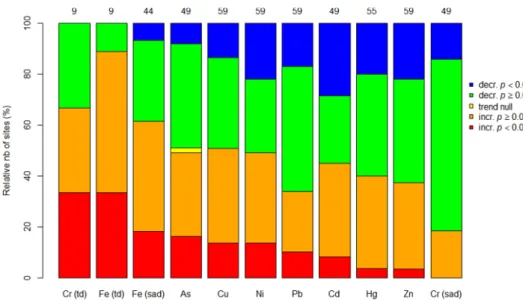
Assessing temporal evolution of TEs in sediments has been limited with increases/decreases in concentrations specific to the local condi-tions and the TEs monitored (e.g. Rainbow et al., 2011; Tappin and Millward, 2015; Traven et al., 2015; Cossa et al., 2018; Kang et al., 2018). In contrast, our database enables site-specific interrogation, but then combines multiple sites to assess broad scale changes. (S1 Table 2 provides the site-specific information enabling a more spatially focused exploration and interrogation of the sites, estuaries, harbours and sub regions monitored for the temporal evolution of nine TEs). Using a minimum of six years of monitoring effort per site, 500 median re-gressions were performed across 69 sites (Fig. 3). Depending on the TE and extraction techniques, between 9 (Fe [td] and Cr [td]) and 59 sites (Zn, Cu, Ni, Pb) were analysed generating decreases, increases and one regression for As showing no temporal change (slope = 0). Globally, 44% of the site/TE regressions showed an increasing trend and 10% with p < 0.05, but at the same time 56% showed decreasing trends and 17% with p < 0.05. Generally, Fe (both extraction techniques) and Cr total extraction, have the majority of sites with increasing trends (accepting the number of sites for each was low). A second cluster (Cu, Ni and As) has close to equal percentages for sites increasing and decreasing, with Ni having a higher percentage of sites with decreasing trends with p < 0.05. Cd, Hg, Zn, Pb and Cr extracted with strong acids form a more varied final cluster where the majority of sites have decreasing trends with 17% to 29% of these with p < 0.05. Nevertheless, Cd, Hg, Zn and Pb still have a small percentage of sites with increasing trends with p < 0.05.

The data presented in Fig. 2 show that at the broadest regional scale some TEs are increasing (e.g. Ni, Fe and Cu), but when viewed with Fig. 3 the site-specific increases are not ubiquitous. Conversely, for Cd, Hg, As, Pb, Zn and Cr, where the broad scale regional analysis shows little change over time regardless of the pollution level, many increasing and decreasing site trends with p < 0.05 are present. The proportions of sites with increasing and decreasing trends with p < 0.05 combined for Cu and Zn, are equivalent when compared to those reported by OSPAR (2015) for ecoregions III and IV (Greater North Sea and Celtic Sea, respectively). However, for all others (Cr and Fe were not compared) our analysis has between two (As) and seven (Pb) times as many sites with increasing trends and two (Pb) and six times (Cd) as many sites with decreasing trends when compared to OSPAR (2015). In addition, 8% of our sites had an increasing trend for Cd, whilst no sites were recorded as increasing by OSPAR (2015). Whilst the significant value of the OSPAR sampling programmes should be recognized, these disparities highlight the importance of having sufficient fine-scale inshore monitoring, reinforcing the importance of replicated monitoring within integrated

Fig. 3. Relative proportions of sites monitored for each TE over a minimum of six years, which show a net increase (incr. p < 0.05, red) or decrease (decr. p < 0.05, blue), an increase (incr.

p ≥ 0.05, orange) or decrease (decr. p ≥ 0.05,

green) or no evolution (trend null, yellow) of their sediment TE concentrations. Numbers above bars are number of sites included in the median regression analysis. Digestion techniques: strong acid digestion (sad) or total digestion (td) are specified and considered separately for Cr and Fe. (For interpretation of the references to colour in this figure legend, the reader is referred to the web version of this article.)

coastal and biological observation networks that can focus on the local, but also provide the foundation for assessing broad-scale changes (She et al., 2019).

3.5. Pollution sources

Reducing marine TE contamination is essential for healthy coastal ecosystems; this drives the comprehensive policy and regulatory frameworks to achieve unpolluted seas. However, despite some re-ductions, data from Figs. 2 and 3 confirm that elevated TE pollution at sites has exerted effects on the benthos via the sediment matrix and bioaccumulation for the period 1981–2013. It may seem disheartening to think that TE persistence should constrain our ability to improve benthic systems, however, as 135 of 500 trends (both positive and negative) in the sediment concentrations had p < 0.05 (Fig. 3), with proportionally more decreases (17%) than increases (10%) change does happen. Change is also reflected at the regional level as shown by the multi-element index and Igeo values (Figs. 1 and 2). Together they confirm that, despite TE persistence, future contamination levels can improve.

Critical to reducing TE concentrations in sediment is an accurate and up to date assessment of the input sources. Whilst significant data have been collected through a multitude of national and international pro-grammes it is recognized some TE inputs are not monitored (e.g. Fe), whilst there is low confidence in some data (GESAMP, 2015; EEA, 2019). We have, therefore, highlighted the main sources that may elucidate the temporal evolution of each TE. Using the data from S1 Table 2, managers can also explore local input sources that may be key drivers for temporal change at the site, estuary, harbour and sub-region scales.

Regional and continental Pb inputs from the atmosphere (Pacyna et al., 2009; OSPAR, 2015; Richmond et al., 2020), rivers (Tappin and Millward, 2015; OSPAR, 2019b) and direct discharges (OSPAR, 2019b) have all declined considerably in the last 35+ years. Concentrations in biota (Raimundo et al., 2011) and sediments (Cossa et al., 2018) have also seen significant reductions. Pb phase out from gasoline has been the main driver, but other direct industrial inputs have also declined (Pacyna et al., 2009). This supports the relatively high number of sites (17% of these with p < 0.05) with decreasing trends (Fig. 3). Never-theless, Rusiecka et al. (2018) reported northeast Atlantic surface water concentrations to still be significantly elevated, implicating long dis-tance transport. Long range circulation (1,000s of kms) and resus-pension from sediments could explain the latter stabilization of the Igeo score (Fig. 2).

Generally, Hg marine inputs and concentrations in sediment and biota have all declined significantly (Pacyna et al., 2007, 2009; Tappin and Millward, 2015; Obrist et al., 2018; OSPAR, 2019a; Richmond et al., 2020). Nevertheless, riverine inputs and direct discharges have stabi-lized in some European countries (OSPAR, 2019b) and increasing at-mospheric loads are reported in Asia (Obrist et al., 2018). Global vigilance is, therefore, required to maintain the declines from the mid- 2000s onwards (Fig. 2) and increase the number of sites with signifi-cantly decreasing trends (Fig. 3).

Cd is also seen as a success story with significant declines in atmo-spheric and riverine inputs aligning to the decline in Igeo score in the 1990s (Fig. 2). Subsequent reductions have been limited (Pacyna et al., 2007, 2009; Tappin and Millward, 2015; OSPAR, 2015; Richmond et al., 2020) and concomitant reductions in biota and sediment have also stalled in some locations (Johnstone et al., 2016). This is reflected in our data where the Igeo score since mid-1990s has failed to reduce further. This highlights the need to increase efforts locally, nationally and globally on key current sources: e.g. combustion of fuel and fertilizer use (OSPAR, 2008; Richmond et al., 2020).

In Europe, direct and riverine Zn discharge levels vary between countries, however, a general decline can be detected (OSPAR, 2019a). Atmospheric emissions for the UK have also declined, but with no

further reductions from the mid-2000s (Defra and BEIS, 2019). The 5- year mean regional Igeo score (Fig. 2) has remained low after re-ductions in the early 1990s and combined with the low number of sites with significantly increasing trends (Fig. 3) would indicate that im-provements have been maintained. Nevertheless, relatively large inputs from current sources including buildings, vehicle emissions, combustion (see Davis et al., 2001; Duan and Tan, 2013) as well as contributions from ‘hidden’ inputs (e.g. anti-fouling paints and anodes (see section below) will make any further reductions very challenging to achieve.

Input data for As are relatively sparse as they are not collated for direct and riverine discharges (OSPAR, 2019a). However, Pacyna et al. (2009) supported by Harmens et al., (2007) show clear reductions in European emissions from the 1950s. Non-ferrous smelting and fossil fuel production are the main sources globally of anthropogenic arsenic, with the replacement of coal burning by natural gas a major factor in the 4- fold decline in UK emissions since 1970 (Faust et al., 2016). Although, the 5-year average regional Igeo score has remained low after a peak in the early 1990s (Fig. 2), relatively high numbers of sites with increasing trends (p < 0.05) (Fig. 3) require further investigation and could mirror local scale changes as reported by Kang et al. (2018).

Cr input data are sparse for similar reasons to As, but domestic and industrial effluents and fuel combustion are identified as key sources (Pacyna et al., 2009; Cheng et al., 2014). The 5-year average regional Igeo score for Cr (sad) increased from the mid-1990s to mid-2000s (Fig. 2), but a subsequent decline would suggest that inputs are stable and this is supported by Kang et al. (2018). However, the high numbers of significantly increasing trends per site (Fig. 3) for the more recent sediment total digestion offset the more important proportion of sites showing significant decreases for strong acid digestion techniques. Cr requires further investigation at the local scale as increases have been associated with point sources including oil installations ( Celis-Hernan-dez et al., 2018) and the metallurgic industry (Cheng et al., 2014).

Anthropogenic activities (combustion; mining and smelting) may have led to a tripling of atmospheric soluble Fe ocean deposition since the industrial revolution (Ito, 2015; Myriokefalitakis et al., 2015). Fe is not routinely measured in sediments, but the increasing Igeo score (Fig. 2) support these input increases. Increasing Fe concentrations may have contradictory effects on sediment toxicity. Firstly, Fe oxides reduce TE bioavailability and consequent toxicity (Xiangdong et al., 2001). However, increases in Fe sediment concentration could have direct impacts, as Johnson et al. (2017) ranked it as 8/60 for toxicity. Exper-imentally investigating the effects of Fe on benthic species is, therefore, essential. Finally, the increase in Fe may also impact all coastal habitats. Dissolved FeII _{is an essential and limiting nutrient that stimulates} pri-mary productivity (e.g. Smetacek et al., 2012). Like other TEs, sediment- bound Fe can be resuspended (Kalnejais et al., 2010). Under these conditions it could be converted to FeII, thus sediment-derived Fe could be a significant driver in the increasing global problem of harmful algal blooms (Smetacek and Zingone 2013).

Anthropogenic sources dominate Ni release (Clayton and Clayton, 1981; Pacyna et al., 2007, 2009; Strincone et al., 2013). Although offi-cial European emissions data suggest a 55% reduction between 1995 and 2000 (Ilyin et al., 2006), measurements in mosses did not show significant recent reductions (Harmens et al., 2007). National and trans- national assessments are required to contextualize the increasing Ni Igeo score from Fig. 2, but also at the site level to identify local inputs. Cempel and Nikel (2006) stated waste water effluents to be major ma-rine inputs, but increased emissions from shipping (Turner et al., 2017) could be key (see section below). A continuation of these inputs will take the Igeo score across the moderately polluted threshold, and although DeForest and Schlekat (2013) indicate Ni has relatively low toxicity, studies on benthic species via sediment exposure are very limited.

Like Zn, direct and riverine discharges of Cu in Europe are highly variable across countries (OSPAR, 2019b). Harmens et al. (2007) did report a significant decreasing trend for concentrations in European moss (1995–2000), but atmospheric emissions for the UK are only

Environment International 149 (2021) 106362 8 Table 2

Assessment of TE inputs (t) year−1 _{into different regions/countries from AF (antifouling paints), scrubbers (vessel exhaust cleaning systems) and anodes (sacrificial hull anodes) with direct and river discharges for the} Channel region and UK (2015), and atmospheric inputs for UK (2018) included for comparison. Values are realistic (mean), minimum and maximum scenarios in parentheses, except OSPAR data which are sometimes given as ranges. Data for 2040 based on predicted changes to vessel numbers and installation/use of scrubbers. See S2 Tables 1–6 for details of each component calculation and supporting references, except OSPAR (2019b, c) and atmospheric inputs (Richmond et al., 2020). For details of vessel types and counting methods for each source category/input region, see S2 Table 2.

Method Source Input region 2020

Cu 2040 Cu 2020 Zn 2040 Zn 2020 Ni 2040 Ni

AF All vessels Solent 94 (3–378) 135 (3–678) 27 (0.7–128) 39 (0.8–231) – –

Scrubbers Merchant vessels (AIS only) Solent 0.4 (0.03–2) 5 (0.3–27) 0.8 (0.02–3) 9 (0.3–30) 0.2 (0.02–0.6) 2 (0.2–7)

Anode All vessels Solent – – 349 (227–490) 503 (271–880) – –

AF All vessels (AIS only) Channel 22 (0.6–102) 32 (0.7–184) 6 (0.1–35) 9 (0.2–62) – –

Anode All vessels (AIS only) Channel – – 82 (46–133) 119 (55–238) – –

Scrubbers Merchant vessels (AIS only) Channel 5 (0.3–28) 58 (0–306) 10 (0.3–31) 107 (0–344) 2 (0.3–7) 24 (0–77)

OSPAR Direct UK Channel 0.25 – 0.24 – – –

OSPAR Direct France + UK Channel 0.25 (- + 0.25) – 0.24 (- + 0.24) – – –

OSPAR Riverine UK Channel 17 – 68 – – –

OSPAR Riverine France + UK Channel 57–59 – 258–259 – – –

OSPAR Riv. + Dir. UK UK 296–338 – 1,028–1,184 – – –

Atmospheric UK UK 269 – 460 – 98 –

AF Recreational vess. UK 340 (15–1,011) 310 (5–1,526) 98 (4–344) 89 (1–519) – –

Anode Recreational vess. UK – – 908 (476–1,362) 828 (144–2,053) – –

AF Recreational vess. Europe 3,624 (159–10,778) 3,307 (48–16,255) 1,041 (39–3,665) 950 (11–5,526) – –

Anode Recreational vess. Europe – – 9,671 (5,069–14,507) 8,825 (1,531–21,876) – –

AF Recreational vess. USA 9,828 (431–29,230) 8,968 (130–44,085) 2,823 (105–9,938) 2,576 (32–14,989) – –

Anode Recreational vess. USA – – 26,228 (13,746–39,342) 23,933 (4,151–56,365) – –

AF Recreational vess. World 19,627 (861–58,371) 17,909 (260–88,036) 5,637 (211–19,846) 5,144 (64–29,932) – –

Anode Recreational vess. World – – 52,376 (27,450–78,564) 47,793 (8,290–118,474) – –

AF Merchant vess. World 1,711 (51–6,408) 2,505 (63–10,563) 491 (12–2,178) 719 (15–3,591) – –

Anode Merchant vess. World – – 6430 (4,213–7,243) 9,414 (5,161–13,095) – –

Scrubbers Merchant vess. World 397 (28–1,797) 4,307 (31–19,917) 728 (25–2,027) 7,898 (278–22,459) 164 (21–451) 1,777 (236–5,004)

J.

Richir

et

declining minimally (Defra and BEIS, 2019). Concentrations in biota (OSPAR, 2016) and sediments have seen increasing trends from multiple sites (OSPAR, 2016; Kang et al., 2018). Cu is used in many applications including: fertilizers (Jensen et al., 2016); vehicle brakes (Davis et al., 2001) and also combustion processes (Bhuiyan et al., 2018). Although brake wear is responsible for the vast majority of the UK’s atmospheric emissions, it has remained relatively constant (e.g. around 200 t y−1 _for 30 years in the UK) (Richmond et al 2020). This and the decline/regu-lation of industrial uses indicate that other sources are driving the increasing regional Igeo score since the 1990s (Fig. 2), but also site- specific changes (Fig. 3).

3.6. ‘Hidden’ sources: Antifouling paints, scrubbers and anodes

For Cu, Ni and Zn a number of rarely-studied sources could be sig-nificant contributors to the sediment concentration evolution. Table 2 values are based on robust empirical data combined with selected literature (S2 Tables 1–6) generating realistic (i.e. mean) inputs with minimum and maximum scenarios reflecting source data variability. Since the Tri Butyl Tin-AF coatings ban, Cu-based AF (and combined with Zn-based products too) now dominate (Amara et al., 2018). Using our Google maps Solent vessel count combined with the other data (see S2 Tables 1–4) the realistic (mean) amount of Cu released is 94 t y−1_. This is double that reported by OSPAR (2019b) for the whole of the Channel region from both riverine and direct discharges and is a third of all UK-wide direct and riverine discharges. In contrast, Solent input levels of Zn are much lower (27 t y−1_{), but still represent 10% of the Zn} entering the Channel region from both France and UK (Table 2). The discrepancy in the amounts calculated for the Solent and Channel region is due to the vessel count method as the AIS data greatly underestimate the number of vessels per region. In coastal areas this is likely to be due to most vessels not having a legal requirement for AIS data transmission (Cope et al., 2020) or turning off the system to preserve battery life (C. Thisby, pers. comm.). At the larger spatial scales Cu and Zn amounts are substantial, but still likely to be significant underestimates due to limited recreational boat and global merchant fleet data. By 2040 the predicted increase in the merchant vessel fleet (a mean of 1.8% y−1_{, S2} Table 1) not surprisingly generates substantial increases for AF inputs globally, but applying a predicted − 0.3% y−1 _{contraction of the USA} recreational fleet to all other regions sees concomitant declines. Nevertheless, recreational boats contribute an order of magnitude more Cu and Zn than the merchant fleet.

Shipping contributes significant emissions to coastal environments (e.g. Aulinger et al., 2016; Xiao et al., 2018) and in response to legis-lation (IMO, 2008a), there has been a noteworthy increase in scrubber installations (Turner et al., 2017). A few studies have directly measured the metal concentrations in scrubber discharge water (see references in S2 Table 5), but no scale-up has been attempted. Although TE concen-trations in waste water are high (see S2 Table 5), the small proportion of merchant vessels (current estimate: 3.4%) fitted with scrubbers and that merchant vessels make up a small fraction of those counted in the Solent means that, in comparison to AF, the amounts of Cu, Zn and Ni dis-charged are low. At the local (Solent) level, scrubber discharge contri-bution to the TE sediment concentrations is, therefore, small and orders of magnitude lower than AF. However, within the Channel and globally, scrubbers contribute nearly double the Zn from AF and 25% of the Cu. The future percentage of vessels fitted with scrubbers is a topic of intense discussion with divergent business responses for embracing scrubber technology. If an industry prediction of 25% by 2040 (S2 Table 5) in conjunction with the yearly increase in merchant fleet size does tran-spire, scrubbers will contribute nearly double the Cu from AF for the global merchant fleet and > 10x the amount of Zn. Globally, Ni inputs will also increase from 164 t in 2020 to 1,777 t in 2040.

Finally, the dissolution of sacrificial metal anodes are intrinsic to boat protection. Only a very limited number of studies have calculated Zn inputs (see references in S2 Table 6) and these were at the very local

level (e.g. Rees et al., 2017) or outdated (e.g. Boxall et al., 2000). At all spatial scales and for all vessel types, inputs of Zn from anodes are an order of magnitude greater than equivalent AF sources. For example, anodes from the UK recreational fleet release 908 t of Zn per year, compared to 98 t from AF. The level of input is equivalent to that re-ported by OSPAR (2015) for direct and riverine discharges for the whole of the UK and similar to a recent calculation by Rees et al. (2020). Despite the predicted contraction in fleet size, recreational vessels will continue to deliver considerable quantities of Zn in 2040 from anodes. However, the input of Zn from scrubbers for the global merchant fleet becomes equally important due to the increase in the predicted pro-portion of the fleet fitted with open scrubbers.

Table 2 clearly shows that inputs of Cu (AF) and Zn (AF, anodes) are already substantial at multiple spatial scales. The Cu Igeo score increase (Fig. 2) is, therefore, supported by the dominance of Cu-based AF coatings on vessels and is highly likely to contribute to the increases in median TEPI and PI values for 2010–2013 (Fig. 1). This is also reinforced by the fact that 88% of the sites with increasing Cu concentrations (p < 0.05) were transitional/coastal water, close to urban areas with sub-stantial vessel numbers. However, S1 Table 2 shows that spatial con-sistency of each TE’s temporal evolution (i.e. multiple sites located within a harbour/estuary/sub-region showing consistent trends) is not always evident. For example, across 20 sites in the Solent both increasing and decreasing trends for Cu are present. A much more detailed local input analysis combined with an understanding of com-plex hydrodynamic and sedimentation processes will be required to fully contextualise the contribution of diffuse versus local (e.g. point dis-charges) sources. Regardless of the local level complexity, non-toxic AF coatings or other AF fouling control methods (e.g. cleaning and fouling waste capture) should be considered a priority for legislators to address these substantial and pervasive inputs (e.g. Bergman and Ziegler, 2019). Although the overall inputs of Zn are much higher due to the contribution from anodes, it is not immediately clear why a lower pro-portion of trends show increases with p < 0.05 (Fig. 3) and the Igeo score (Fig. 2) remains fairly constant. Declines in UK atmospheric emissions (Defra and BEIS, 2019) may have been counteracted by the AF and anode inputs, but legislation to expedite appropriate cleaning control along with education for recreational vessel owners on anode use would be important first steps (Rees et al., 2017). The increasing Igeo score for Ni is more challenging to explain based on the relatively low scrubber inputs for the Solent (0.2 t y−1_{) and the Channel (2 t y}−1_{) from Table 2.} Extensive burning of higher sulphur fuel oil by the majority of merchant vessels generates significant Ni atmospheric emissions (e.g. Peltier and Lippmann, 2010; Zhao et al., 2013). These would be deposited to the marine environment and concentrated by hydrodynamic currents to more localised areas (see S1 Table 2), although unknown point sources may also be responsible for spatial inconsistencies. Our data predict that scrubber discharges could be a significant future direct input source of Ni (as well as Zn and Cu and other TEs) to marine environments, which requires waste water discharges to be regulated for metals (rather than just guidelines at present IMO, 2008b). However, unless there is a much more rapid conversion to low sulphur (or alternative) fuels, Ni and other metals will still continue to input the marine environment, but indirectly from atmospheric deposition.

4. Conclusions

Mining sediment contamination databases from national public sources is a powerful tool to assess the contamination evolution at scales that are challenging to address. Integration within coastal observatory networks will significantly enhance their value and application, enabling managers to link ecosystem management approaches with multiple TE contamination levels that together have significant cumu-lative effects. However, this will require investment in data alignment and quality processes supported by long term monitoring of sufficient sentinel sites.

Environment International 149 (2021) 106362 Our long-term spatiotemporal analysis identifies considerable

im-provements in contamination (declining TEPI and PI) at the regional level since the 1980s. Nevertheless, the increase in TEPI and PI for 2010–13, increasing Igeo scores for Cu, Fe and Ni; stabilization of other TE Igeo scores after declines (Cd, Zn, Hg, Pb) combined with the numbers of sites that have increasing trends all indicate continued/increasing inputs. Accurate input assessments including ‘hidden’ sources are, therefore, urgently required especially in the context of the global focus on the blue economy (e.g. UN Decade of the Oceans) and predicted in-creases in shipping, coastal aquaculture, marine electricity generation etc. to support growth (OECD, 2016). Ultimately, this must inform appropriate legislation and control measures to protect ecologically and economically valuable benthic systems across the globe.

CRediT authorship contribution statement

Richir Jonathan: Conceptualization, Data curation, Formal anal-ysis, Investigation, Methodology, Supervision, Validation, Visualization, Writing - original draft, Writing - review & editing. Bray Simon: Methodology, Validation, Writing - review & editing. McAleese Tom: Data curation, Formal analysis, Investigation. Watson J. Gordon: Conceptualization, Data curation, Formal analysis, Funding acquisition, Investigation, Methodology, Project administration, Resources, Super-vision, Validation, Visualization, Writing - original draft, Writing - re-view & editing.

Declaration of Competing Interest

The authors declare that they have no known competing financial interests or personal relationships that could have appeared to influence the work reported in this paper.

Acknowledgements

The TE data were provided by the EA (C. Ashcroft) and the BODC (A. Bargery and J. Ayliffe). BODC supplied data on behalf of the Clean Safe Seas Evidence Group, collected by: a) Agri-Food and Biosciences Insti-tute, b) Centre for Environment, Fisheries and Aquaculture Science, c) Department of Agriculture, Environment and Rural Affairs, d) Envi-ronment Agency, e) Food Standards Scotland, f) Marine Scotland Sci-ence, g) Natural Resource Wales and h) Scottish Environment Protection Agency. BODC data were funded by a), c), and the Scottish Govt. Data contain public sector information licensed under the Open Government Licence v3.0. http://www.nationalarchives.gov.uk/doc/open-govern-ment-licence/version/3/. Authors thank D. McMannus, M. Anfield and the marina survey responders for their contributions. This European Regional Development funded work was performed in the framework of the Channel Catchments Cluster (3C) programme.

Appendix A. Supplementary material

Supplementary data to this article can be found online at https://doi. org/10.1016/j.envint.2020.106362. The geo-spatial information con-tained in geographic KML files enables the visualization of sites from their geolocalisation on Google Earth.

References

Amara, I., Miled, W., Slama, R.B., Ladhari, N., 2018. Antifouling processes and toxicity effects of antifouling paints on marine environment: a review. Environ. Toxicology and Pharm. 57, 115–130.

Aulinger, A., Matthias, V., Zeretzke, M., Bieser, J., Quante, M., Backes, A., 2016. The impact of shipping emissions on air pollution in the greater North Sea region–Part 1: current emissions and concentrations. Atmos. Chem. Phys. 16, 739–758. Bengtsson, H., 2020. matrixStats: Functions that Apply to Rows and Columns of Matrices

(and to Vectors). R package version 0.56.0. https://CRAN.R-project.org/package =matrixStats.

Bergman, K., Ziegler, F., 2019. Environmental impacts of alternative antifouling methods and use patterns of leisure boat owners. Int. J. Life Cycle Ass. 24, 725–734.

Beyer, J., Green, N.W., Brooks, S., Allan, I.J., Ruus, A., Gomes, T., Bråte, I.L.N., Schøyen, M., 2017. Blue mussels (Mytilus edulis spp.) as sentinel organisms in coastal pollution monitoring: a review. Mar. Env. Res. 130, 338–365.

Bhuiyan, M.K.A., Qureshi, S., Billah, M.M., Kammella, S.V., Alam, M.R., Ray, S., Monwar, M.M., Abu Hena, M.K., 2018. Distribution of trace metals in channel sediment: a case study in south Atlantic coast of Spain. Water Air Soil Pollut. 229, 1–14.

Birch, G.F., 2017. Determination of sediment metal background concentrations and enrichment in marine environments–a critical review. Science of Tot. Environ. 580, 813–831.

Borchers, H.W., 2019. pracma: Practical Numerical Math Functions. R package version 2.2.9. https://CRAN.R-project.org/package=pracma.

Boxall, A.B.A., Comber, S.D., Conrad, A.U., Howcroft, J., Zaman, N., 2000. Inputs, monitoring and fate modelling of antifouling biocides in UK estuaries. Mar. Pollut. Bull. 40, 898–905.

Brady, J.P., Ayoko, G.A., Martens, W.N., Goonetilleke, A., 2015. Development of a hybrid pollution index for heavy metals in marine and coastal sediments. Environ. Monit. Assess. 187, 306.

Bryan, G.W., Langston, W.J., 1992. Bioavailability, accumulation and effects of heavy- metals in sediments with special reference to United Kingdom Estuaries - a review. Environ. Pollut. 76, 89–131.

Cade, B.S., Noon, B.R., 2003. A gentle introduction to quantile regression for ecologists. Front. Ecol. Environ. 1, 412–420.

Caplat, C., Texier, H., Barillier, D., Lelievre, C., 2005. Heavy metal mobility in harbour contaminated sediments: the case of Port-en-Bessin. Mar. Pollut. Bull. 50, 504–511. CCME, 2001. Canadian Council of Ministers of the Environment. Canadian sediment

quality guidelines for the protection of aquatic life: Summary tables. Updated. In: Canadian environmental quality guidelines, 1999, Canadian Council of Ministers of the Environment, Winnipeg.

Celis-Hernandez, O., Rosales-Hoz, L., Cundy, A.B., Carranza-Edwards, A., Croudace, I.W., Hernandez-Hernandez, H., 2018. Historical trace element accumulation in marine sediments from the Tamaulipas shelf, Gulf of Mexico: an assessment of natural vs. anthropogenic inputs. Science of Tot. Environ. 622–623, 325–326.

Cempel, M., Nikel, G., 2006. Nickel: a review of its sources and environmental toxicology. Pol. J. Environ. Stud. 15, 375–382.

Cefas, 2012. CSEMP Green Book. http://cefas.defra.gov.uk/media/510362/greenboo kv15.pdf.

Cheng, H., Zhou, T., Lui, Q., Lu, L., Lin, C., 2014. Anthropogenic chromium emission in China from 1990 to 2009. Plos one 9, e87753.

Clayton, G.D., Clayton, F.E., 1981. Patty’s Industrial Hygiene and Toxicology. Vol. 2A. Toxicology. John Wiley & Sons, Inc., UK, pp. 1467–2878.

Cook, J.M., Gardner, M.J., Griffiths, A.H., Jessep, M.A., Ravenscroft, J.E., Yates, R., 1997. The comparability of sample digestion techniques for the determination of metals in sediments. Mar. Pollut. Bull. 34, 637–644.

Cope, S., Hines, E., Bland, R., Davis, J.D., Tougher, B., Zetterlind, V., 2020. Application of a new shore-based vessel traffic monitoring system within San Francisco Bay. Front. Mar. Sci. 7, 86.

Cossa, D., Fanget, A.S., Chiffoleau, J.F., Bassetti, M.A., Buscail, R., Dennielou, B., Briggs, K., Arnaud, M., Gu´edron, S., Bern´e, S., 2018. Chronology and sources of trace elements accumulation in the Rhˆone pro-delta sediments (Northwestern Mediterranean) during the last 400 years. Prog. Oceanog. 163, 161–171.

Davis, A.P., Shokouhian, M., Ni, S., 2001. Loading estimates of lead, copper, cadmium, and zinc in urban runoff from specific sources. Chemosphere 44, 997–1009.

DeForest, D.K., Schlekat, C.E., 2013. Species sensitivity distribution evaluation for chronic nickel toxicity to marine organisms. Integr. Environ. Asses. 9, 580–589. Defra and BEIS. via naei.beis.gov.uk (accessed 2019).

Duan, J., Tan, J., 2013. Atmospheric heavy metals and arsenic in China: situation, sources and control policies. Atmos. Environ. 74, 93–110.

Dung, T.T.T., Cappuyns, V., Swennen, R., Phung, N.K., 2013. From geochemical background determination to pollution assessment of heavy metals in sediments and soils. Rev. Environ. Sci. Bio. 12, 335–353.

EEA, 2019. Contaminants in Europe’s seas. Moving towards a clean, non-toxic marine environment: Report by the European Environment Agency, pp.61.

EU, 2000. Directive 2000/60/EC of the European Parliament and of the Council of 23 October 2000 establishing a framework for Community action in the field of water policy as amended by Decision 2455/2001/EC and Directives 2008/32/EC, 2008/ 105/EC and 2009/31/EC.

Farrington, J.W., Tripp, B.W., Tanabe, S., Subramanian, A., Sericano, J.L., Wade, T.L., Knap, A.H., 2016. Edward D. Goldberg’s proposal of “the mussel watch”: reflections after 40 years. Mar. Pollut. Bull. 110, 501–510.

Faust, J.A., Junninen, H., Ehn, M., Chen, X., Ruusuvuori, K., Kieloaho, A.J., Back, J., Ojala, A., Jokinen, T., Worsnop, D.R., Kulmala, M., 2016. Real-time detection of arsenic cations from ambient air in boreal forest and lake environments. Environ. Sci. Technol. Lett. 3, 42–46.

GESAMP, 2015. IMO/FAO/UNESO-IOC/UNIDO/WMO/IAEA/UNEP Joint group of experts on the Scientific Aspects of Marine Environmental Protection. Pollution in the Open Oceans 2009–2013 – a report by a GESAMP Task TEAM. Boelens R. and Kershaw P.J. 91, 87.

Gosling, E., 1992. The Mussel Mytilus: Ecology, Physiology, Genetics and Culture. Elsevier, Netherlands, p. 602.

Hall, G.E., 2017. Determination of trace elements in sediments. In: Manual of Physico- Chemical Analysis of Aquatic Sediments. Routledge, UK, pp. 85–145.

Harmens, H., Norris, D.A., Koerber, G.R., Buse, A., Steinnes, E., Rühling, Å., 2007. Temporal trends in the concentration of arsenic, chromium, copper, iron, nickel,