Application of deterministic and stochastic analysis to calculate a stadium with pressure measurements in wind tunnel
Texte intégral
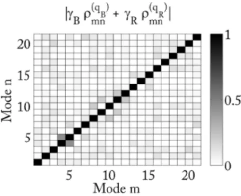
Figure
Documents relatifs
We can distinguish three types of reactivity yields: very low reactivity (2 –3 %) corresponding to initial structures in which the proton is located on the formyl group
There are several caveats to these results (the first few affecting many other similar studies). 1) Many deaths occur outside of hospitals, hence the dire deaths estimates of the
- Dans son rapport annuel 2001-2002 sur l’état et les besoins de l’éducation, le Conseil supérieur de l’éducation propose à la société québécoise deux grandes
Et tu contemples ces vastes cieux Toute ta vie s'est passée dans la gloire De voir ton cœur doux comme ce soir De te relier avec tout ce qui fait un
We have defined a first version of a plant breeding API that defines the key calls needed to exchange information about germplasm, phenotypes, experiments, studies, geographic
236 Fig-4.48: Accumulated glutamine consumption and ammonia concentration profiles of the hybridoma cultures using enriched medium and sodium butyrate in the presence
Dans le travail n°1, nous avons montré la faisabilité de détecter l’ADNtumc par dPCR directement à partir du plasma de 43 prélèvements de patients avec
regression model was found to successfully predict the wett- ability of the materials within the polymer microarray from the concatenated positive and negative spectra acquired from
